Optimizing Gershgorin for Symmetric Matrices
Abstract
The Gershgorin Circle Theorem is a well-known and efficient method for bounding the eigenvalues of a matrix in terms of its entries. If is a symmetric matrix, by writing , where is the matrix with unit entries, we consider the problem of choosing to give the optimal Gershgorin bound on the eigenvalues of , which then leads to one-sided bounds on the eigenvalues of . We show that this can be found by an efficient linear program (whose solution can in may cases be written in closed form), and we show that for large classes of matrices, this shifting method beats all existing piecewise linear or quadratic bounds on the eigenvalues. We also apply this shifting paradigm to some nonlinear estimators and show that under certain symmetries this also gives rise to a tractable linear program. As an application, we give a novel bound on the lowest eigenvalue of a adjacency matrix in terms of the “top two” or “bottom two” degrees of the corresponding graph, and study the efficacy of this method in obtaining sharp eigenvalue estimates for certain classes of matrices.
AMS classification: 65F15, 15A18, 15A48
Keywords: Gershgorin Circle Theorem, Eigenvalue Bounds, Linear Program, Adjacency Matrix
1 Introduction
One of the best known bounds for the eigenvalues of a matrix is the classical Gershgorin Circle Theorem [1, 2], which allows us to determine an inclusion domain of the eigenvalues of a matrix that can be determined solely from the entries of this matrix. Specifically, given an matrix whose entries are denoted by , we define
Then the spectrum of is contained inside the union of the .
If is a symmetric matrix, then the spectrum is real. In general, we might like to determine whether is positive definite, or even to determine a bound on the spectral gap of , i.e. a number such that all eigenvalues are greater than . Let us refer to the diagonal dominance of the th row of the matrix by the quantity . A restatement of Gershgorin is that the smallest eigenvalue is at least as large as the smallest diagonal dominance of any row.
As an example, let us consider the matrix
| (1) |
and we see the quantity for all rows. From this and Gershgorin we know that all eigenvalues are at least , but we cannot assert that is positive definite. However, we can compute directly that ; not only is positive definite, it has a spectral gap of .
We then note that (here and below we use to denote the matrix with all entries equal to ). Since is positive definite and is positive semidefinite, then it follows that is positive definite as well. In fact, we know that the eigenvalues of are at least as large as those of , so that has a spectral gap of at least , which gives us the exact spectral gap.
Let us consider the family of matrices with , and consider how the diagonal dominance changes. Subtracting off the value of from each entry moves the diagonal to the left by , but as long as the off-diagonal terms are positive, it decreases the off-diagonal sum by a factor of . This has the effect of moving the center of each Gershgorin circle to the left by , but decrease the radius by , effectively moving the left-hand edge of each circle to the right by . This gives an improved estimate for the lowest eigenvalue. It is not hard to see in this case that choosing gives the optimal diagonal dominance of 1. Generalizing this idea: let be a symmetric matrix with strictly positive entries. Since is positive semidefinite, whenever , is positive definite whenever is. However, subtracting from each entry, at least until some of the entries become negative, will only increase the diagonal dominance of each row: each center of each Gershgorin circle moves to the left by , but the radius decreases by . From this it follows that we can always improve the Gershgorin bound for such a matrix with positive entries by choosing to be the smallest off-diagonal term.
However, now consider the matrix
| (2) |
We see directly that the bottom row has the smallest diagonal dominance of . Subtracting off a 1 from each entry gives
and now the bottom row has a diagonal dominance of . From here we are not able to deduce that is positive definite. However, as it turns out, for all , the matrix has a positive diagonal dominance for each row, and by the techniques described in this paper we can compute that the optimal choice is :
and each row has a diagonal dominance of . Since is positive semi-definite, this guarantees that is positive definite and, in fact, has a spectral gap of at least . In fact, we can compute directly that the eigenvalues of are , so this it not too bad of a bound for this case.
At first it might be counter-intuitive that we should subtract off entries and cause some off-diagonal entries to become negative, since the is a function of the absolute value of the off-diagonal terms and making these entries more negative can actually make the bound from the th row worse. However, there is a coupling between the rows of the matrix, since we are looking for the minimal diagonal dominance across all of the rows: it might help us to make some rows worse, as long as we make the worst row better. In this example, increasing past does worsen the diagonal dominance of the first row, but it continues to increase the dominance of the third row, and thus the minimum is increasing as we increase . Only until the rows pass each other should we stop, and this happens at . From this argument it is also clear that the optimal value of must occur when two rows have an equal diagonal dominance.
The topic of this paper is to study the possibility of using the idea of shifting the entries of the matrix uniformly to obtaining better eigenvalue bounds. Note that this technique is potentially applicable to any eigenvalue bounding method that is a function of the entries of the matrix, and we consider examples other than Gershgorin as well. We show that using Gershgorin, which is piecewise linear in the coefficients of the matrix, the technique boils down to the simultaneous optimization of families of piecewise linear functions, so can always be solved, e.g. by conversion to a linear program. We will also consider “nonlinear” versions of Gershgorin theorems and shift these as well, but we see that for these cases we can lose convexity and in general this problems are difficult to solve.
We show below that for many classes of matrices, the “shifted Gershgorin” gives significantly better bounds than many of the unshifted nonlinear methods that are currently known.
2 Notation and background
Throughout the remainder of this paper, all matrices are symmetric.
Definition 2.1.
Let be a method that gives upper and lower bounds on the eigenvalues of a matrix as a function of its entries. We denote by as the greatest lower bound method can give on the spectrum of , and by the least upper bound.
Here we review several known methods. There are many methods known that we do not mention here; a very comprehensive and engaging review of many methods and their histories is contained in [2].
-
1.
Gershgorin’s Circles. [1] As mentioned in the introduction, define
Then . For this method, we obtain the bounds
(3) -
2.
Brauer’s Ovals of Cassini. [3], [4, eqn. (21)] Using the definitions of as above, let us define
Then . It can be shown [2, Theorem 2.3] that this method always gives a nonworse bound than Gershgorin (note for example that choosing gives a Gershgorin disk). The bounds come from the left- or right-hand edges of this domain, so that have the same sign. This gives
The roots of this quadratic are
Therefore we have
(4) (5) - 3.
-
4.
Cvetkovic–Kostic–Varga method. Let be a nonempty set of , and , and let
Further define
According to Theorem 6 of [6],
Definition 2.2.
Let be a method as above, and let us define the shifted- method given by
Note that the domain of optimization is in one definition and in the other. For example is the best lower bound that we can obtain by method on the family given by subtracting a positive number from the entries of , whereas is the best upper bound obtained by adding a positive number.
Remark 2.3.
We will focus our study on the first two methods in the interest of brevity, i.e. we consider for Gershgorin and Brauer. However, we present all four above as representative of a truly large class of methods that share a common feature: the bounds are always a function of the diagonal entries and a sum of (perhaps a subset) of the absolute values of the off-diagonal terms on each row. As we show below in Section 3, the shifted bounds are a function not just of sums of off-diagonal terms, but a function of each individual entry. As such, it is not surprising that shifted bounds can in some cases vastly outperform the unshifted bounds — we will see even that shifted Gershgorin can outperform even unshifted nonlinear bounds such as Brauer.
Lemma 2.4.
If is a method that bounds the spectrum of a matrix, then the spectrum of is contained in the interval , i.e. the scaled bounds are good upper and lower bounds for the eigenvalues.
Proof.
The proof of this follows from the Courant Minimax Theorem [7, §4.2], [8, §4]: Let be a symmetric matrix, and let be the eigenvalues, then we have
If we write , then
| (6) |
If , then the second term is zero (in fact, is a rank-one matrix with top eigenvalue ), and thus we have . Since , we have for all ,
and the same is true after taking the supremum. Similarly,
and if , the second term is zero. Therefore, for all ,
and the same remains true after taking the infimum of the right-hand side. ∎
It is clear from the definition that and for any method and any matrix . In short, shifting cannot give a worse estimate, and by Lemma 2.4 this improved estimate is still a good bound. Moreover, as long as
then , and similarly for the upper bounds. Moreover, we show in many contexts that the bounding functions are convex in , so the converse is also true in many cases.
Remark 2.5.
If we reëxamine the proof of Lemma 2.4, we might hope that we could obtain information on a larger domain of shifts; for example, in (6), when , we have , so we have for ,
| (7) |
We might hope that this could give useful information even when , but some calculation can show that (at least for all of the methods described in this paper) the first term on the right-hand side cannot grow fast enough to make the right-hand side of this inequality increase as decreases, so this will always give a worse bound than just restricting to . For example, for Gershgorin, the absolute best case is that all of the signs align and the edge of the Gershgorin disk is moving to the right at rate , but this is exactly counteracted by the second term on the right-hand side of (7).
3 Shifted Gershgorin bounds
In this section, we concentrate on the shifted Gershgorin method. Recall that the standard Gershgorin bounds are given by
Let us define
| (8) |
then
Theorem 3.1.
The main results for the shifted Gershgorin are as follows:
-
•
(Local Improvement.) Iff, for every with , row of the matrix has at least positive numbers, then . Iff, for every with , row of the matrix has at least negative numbers, then .
-
•
(Global bounds.) Each of the functions can be written as a single piecewise-linear function. Alternatively, we can write these functions as cut out by lines, i.e.
(9) where the constants in the above expressions are given in Definition 3.3;
-
•
(Convexity.) It follows from the previous that the functions and are convex, i.e. is “concave down” and is “concave up” in . From this it follows that the minimizer is attained at a unique value, or perhaps on a unique closed interval.
Remark 3.2.
The local improvement part of the theorem above is basically telling us that we have to have enough terms of the correct sign to allow the shifting to improve the estimates. If a row has many more positive terms than negative terms, for example, then subtracting the same number from each entry improves the Gershgorin bound, since it decreases the off-diagonal sum — from this we see that we would want the row(s) which are the limiting factor in the calculation to have enough positive terms. In particular, it follows that if there are enough terms of both signs, shifting can improve both sides of the bound.
One quick corollary of this theorem is that if we have a matrix with all positive entries (or even all positive off-diagonal entries), then shifting is guaranteed to improve the lower bound, yet cannot improve the upper bound. In this sense, our theorem is in a sense a counterpoint to the Perron–Frobenius theorem: the bound on the spectral radius of a positive matrix is exactly the one given by Perron–Frobenius, but we always obtain a good bound on the least eigenvalue.
The global bound part of this theorem tells us that we can write the objective function as a single piecewise-linear function, or as an extremum of at most different linear functions. This more or less allows us to write down the optimal bound in closed form, see Corollary 3.5 below. In any case, the optimal bound can be obtained by a linear program.
Definition 3.3.
Let be an symmetric matrix. We define for . For each , we define as follows: let be the off-diagonal terms of row of the matrix in nondecreasing order, and define, for ,
and then
Finally, we define
Lemma 3.4.
The functions are piecewise linear, and can be written as a minimizer of a family of linear functions:
Proof.
Define as in Definition 3.3. First note that we can write
since the ordering in the sum does not matter. Now, note that if (which could be an empty interval), we have
In the case where , it is easy to see that this equality does not hold on an interval, but it does hold at the point . Finally, noting that and , this means that for all (note the negative sign in front of the sum!). Thus the family dominates , and coincides with it on a nonempty set, and this proves the result.
The argument is similar for . If we write
and the remainder follows by taking maxima. ∎
Proof of Theorem 3.1.
First we prove the “global bounds” part of the theorem. From Lemma 3.4,
and we are done. The proof is the same for .
The argument for convexity is similar. We have
As a minimizer of linear functions, it follows that is concave down, and similarly, as is the maximizer of linear functions, it is concave up.
Finally, we consider the “local improvement” statement. Choose and fix a row , and define as in Definition 3.3. If all of the entries of are positive, then for , , and thus has a positive slope at . Otherwise, let us write . If , then has a positive slope at . Thus, as long as , then has a positive slope at . In short, has a positive slope at zero iff at least of the entries of are positive. Since is the minimum of the , as long as this is true for every row which minimizes the quantity in a neighborhood of zero, then is itself increasing at .
∎
Corollary 3.5.
Let be an symmetric matrix and consider a set of pairs of indices defined by
Then if , then and
| (10) |
and if then . Moreover, the minimum of occurs at , where are chosen so that (10) is minimized. Also, if the (off-diagonal) terms of are all positive, then the set is the set .
Proof.
First note that if the entries of are positive, then for all , and thus . From this it follows that if then , and the last sentence follows.
From Theorem 3.1, in particular (9), it follows that the supremum of will be attained at the intersection of two lines, and moreover it is clear that this must between between a line of nonnegative slope () and a line of nonpositive slope (). Finding the intersection point gives
Since the denominator is positive, we need the numerator be nonnegative, which gives the condition . Plugging this point into the line gives the expression in parentheses in (10). The minimum such intersection gives us our answer. ∎
Example 3.6.
Let be a matrix and compute . Using Corollary 3.5, there are at most only terms to minimize over: and . If is the largest, then we cannot improve the lower bound by shifting, and in fact we obtain . If is the smallest (which will always happen, for example, when the off-diagonal entries of are positive), then we obtain
If we consider from (1), since is independent of , we can obtain from any row, and we have
and thus
Since the minimum was attained by the pair, we have that it is attained at . This matches the analysis in the introduction.
Example 3.7.
Choosing as in (2), we have
so that
Therefore
We also see that we can choose either pair to find the at which this is minimized, using the pair gives at . We could also ask for which the matrix is guaranteed to be positive definite; note that we have
so it is in the domain .
4 Shifted Brauer Bounds
In this section we consider the shifted Brauer estimator. The Brauer estimate is nonlinear and, moreover, we show that the convexity properties of shifted Gershgorin no longer apply. We show that this adds considerable technical difficulty to the problem, except in certain cases. Although we do not study the shift of some of the other nonlinear estimators from Section 2, we see from the difficulties that arise for Brauer that it is unlikely for us to obtain a tractable optimization problem without further assumptions.
We recall from (4) that
and thus
Noting that
and writing
this simplifies to
| (11) |
This last expression is deceptively complicated, because in fact the functions are not convex, or even very simple.
Example 4.1.
In Figure 1 we plot a few examples of to get a sense of the shape of such functions. In each case, we specify the diagonal entry, and the set of off-diagonal entries, of the first two rows of a matrix, and plot . For example, if
we obtain the figures in Figure 1. (Note that as long as we choose the diagonal entries the same, this simply shifts the function without changing its shape.) First note that neither function has the properties from the last section: although the function in the right frame is close to being concave down, it is not quite, and clearly the function in the left frame is far from concave down.
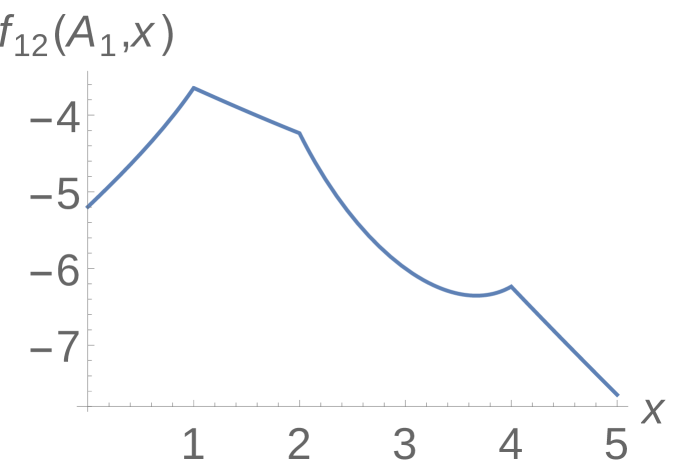
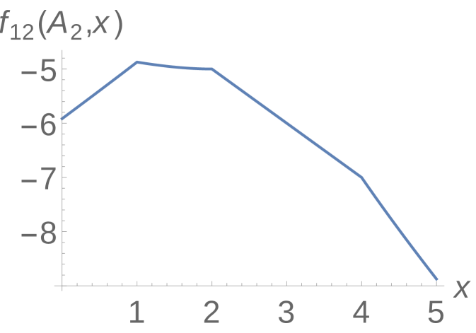
We could, in theory, write out the expression (11) as a single minimization over a large number of functions. Consider the expression for : the expression under the radical is piecewise quadratic on any interval between distinct off-diagonal terms of the two rows, and since , this means that could be written as the minimum of such terms. However, this approach will not be as fruitful as it was in the previous section, since these functions can be both concave up and concave down. Moreover, since the bounding functions are nonlinear with a square root, it is possible that they have a domain strictly smaller than . In any case, extrema do not have to occur at the places where the domain of definition shifts.
However, there is one case where an approximation gives a tractable minimization problem, which we state below.
Theorem 4.2.
Assume that all of the diagonal entries of are the same, and denote this number by . Then if we define
| (12) |
then is still a good lower bound for the eigenvalues of .
Remark 4.3.
Notice that the RHS of (12) is simply the average of the Gershgorin bounds given by the th and th rows. As such, these functions are again piecewise linear and can be attacked in a similar manner to that of the previous section, which we discuss below. Also, notice in the statement of the theorem that we can assume wlog that , since adding to every diagonal entry simply shifts every eigenvalue by exactly .
Proof.
If , then
Notice that
where the are the linear bounding functions from (8). Thus we can define
and we are guaranteed that , so that it is still a good bound for the eigenvalues. ∎
Definition 4.4.
Let be an symmetric matrix with all diagonal entries equal to . Define for . For each , let us define and as follows: let be the nondiagonal entries of rows and of the matrix in nondecreasing order, and then for ,
and finally .
Proposition 4.5.
If the diagonal entries of are all the same, then (q.v. Theorem 3.1)
Proof.
The proof is similar to that of the previous section. The main difference is that while the slope decreases by two every time passes through a non-diagonal entry of row , the slope of decreases by one every time passes through a non-diagonal entry of row or row . From this the potential slopes of can be any integer between and , and everything else follows. ∎
5 Applications and Comparison
In Section 5.1 we use the main results of this paper to give a bound on the lowest eigenvalue of the adjacency matrix of an undirected graph, which is sharp for some circulant graphs. In Section 5.2 we perform some numerics to compare the shifted Gershgorin method to other methods on a class of random matrices with nonnegative coefficients. Finally in Sections 5.3 and 5.4 we consider the efficacy of shifting as a function of many of the entries of the matrix.
5.1 Adjacency matrix of a graph
Definition 5.1.
Let be an undirected loop-free graph; is the set of vertices of the graph and is the set of edges. We define the adjacency matrix of the graph to be the matrix where
We also write if . We define the degree of vertex , denoted , to be the number of vertices adjacent to vertex . We will denote the maximal and minimal degrees of by . We also denote (resp. ) as the second largest (resp. smallest) degrees of .
We use the convention here that for all . This choice varies in the literature but making these diagonal entries to be one instead will only shift every eigenvalue by . From Remark 3.2, since all off-diagonal entries are nonnegative, we have . However, we can improve the left-hand bound by scaling. Intuitively, we expect the scaling to help when there are many positive off-diagonal terms, so we expect this to help best when we have a “dense” graph, i.e. a graph with large .
We can use the formulas from above, but in fact we can considerably simplify this computation. Note that
Notice that this function is decreasing for in any case, so we can restrict the domain of consideration to . Restricted to this domain, the function simplifies to
Noting that , we see that all of these functions are equal to at . From this it follows that the only possible optimal points are in the three cases that all of the slopes are negative, some are of each sign, and all slopes are positive. (The simplest way to see this is to note that the family of lines given by all “pivot” around the point .)
The case where all slopes are negative is if for all , or . In this case, the unshifted Gershgorin bound of is the best that we can do. If not all of the slopes are of one sign, i.e. , then the best bound is . Finally, if all of the slopes are positive, i.e. , then at we obtain the bound .
Noting that all of the diagonal entries of are the same, we can use Theorem 4.2 and consider the . If we define to be the average of the degrees of vertices and , then
If we also define as the average of the two largest degrees of , and as the average of the two smallest degrees, then everything in the previous case analogously holds with replaced by .
Finally, note that we can apply the Brauer method, in a similar manner, directly. Rewriting the above to obtain
we have
Again, we see that all of these functions are equal at and again take value . At , this gives the unshifted Brauer bound of which is of course minimized at . At , we obtain the bound
which is minimized at . As before, the first bound is best for graphs with small largest degree, the second bound is best for graphs with large smallest degree, and the bound is best for graphs with a large separation of degrees.
One can check directly that these bounds are exact for the - and -circulant graphs. Of course when the graph is regular, the Gershgorin and Brauer bounds coincide. In Figure 2 we plot numerical computations for a sample of Erdős–Rényi random graphs. We consider the case with vertices and an edge probability of (we are considering the case where the minimal degree is large, so the shifted bound is best). We see that for a few graphs, this estimate is almost exact, and seems to be not too bad for a large selection of graphs. Note that the unshifted bounds given by either Gershgorin or Brauer are much worse in this case: the average degree of the vertices in these graphs is , and the average maximal degree is larger still (see [9] for more precise statements), so that the unshifted methods would give bounds near , which is much further from the actual values.
5.2 Numerical comparisons of unshifted and shifted methods
Here we present the results of a numerical study comparing methods studied here to the existing methods, where we compare the left bound given by multiple methods for matrices with nonnegative coefficients.
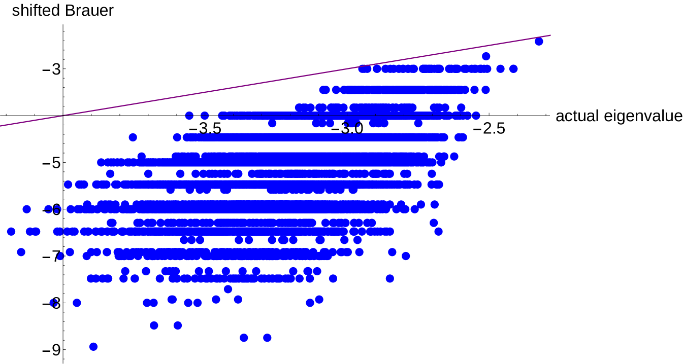
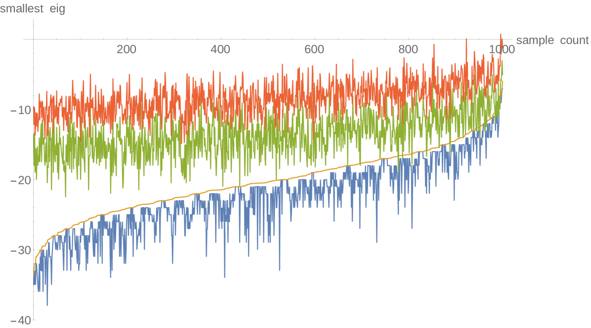
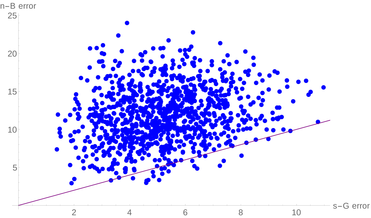
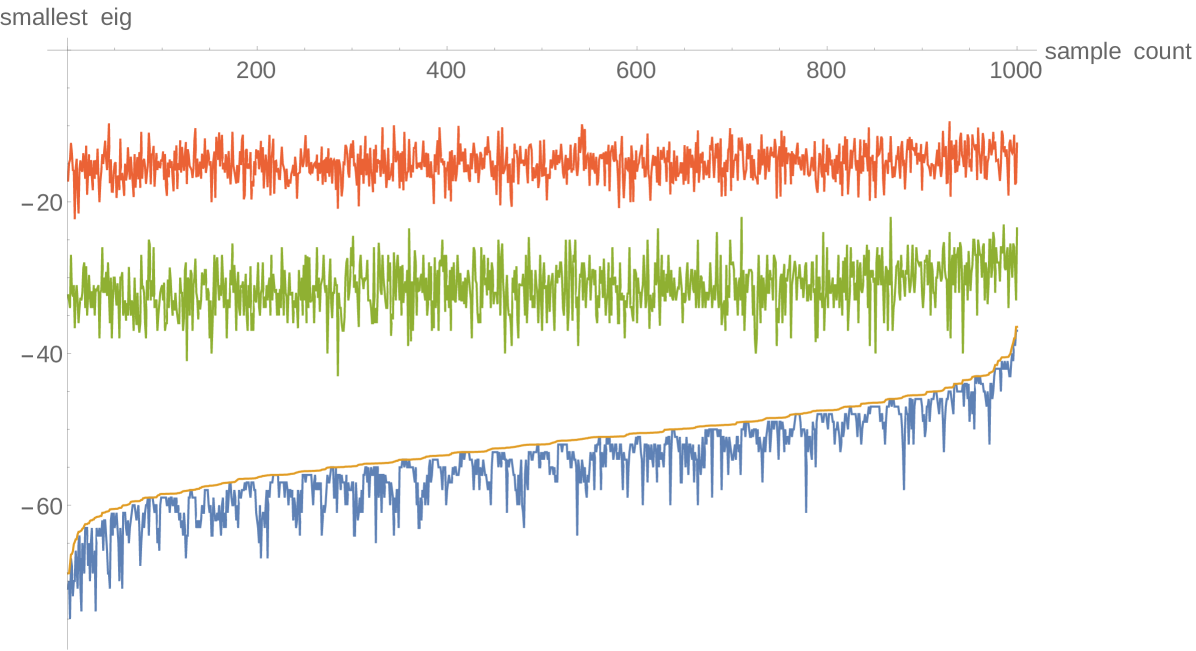
We present the results of the numerical experiments in Figures 3 and 4. In each case, we considered matrices with random integer coefficients in the range . For each random matrix , we compute the unshifted Gershgorin bound , the unshifted Brauer bound , the shifted Gershgorin bound , and the actual smallest eigenvalue. In terms of computation, we computed all of these directly except for , and here we used (9).
In the left frame of each figure, we plot all four numbers for each matrix. Since these are all random samples, ordering is irrelevant, and we have chosen to order them by the value of (yellow). We have plotted in blue, and we confirm in this picture that . Finally, we plot in green and the actual smallest eigenvalue in red. We see that for most samples, and is actually quite a bit better in many cases. We further compare and in Figure 4, where we have a scatterplot of the error given by the two bounds: on the -axis we plot (the error given by shifted Gershgorin) and on the -axis we plot (the error given by unshifted Brauer). We also plot the line for comparison. We again see that shifted Gershgorin frequently beats unshifted Brauer, and typically by quite a lot. In fact, in 1000 samples we found that they were exactly the same 4 times, and unshifted Brauer was better 21 times, so that shifted Gershgorin gives a stronger estimate of the time.
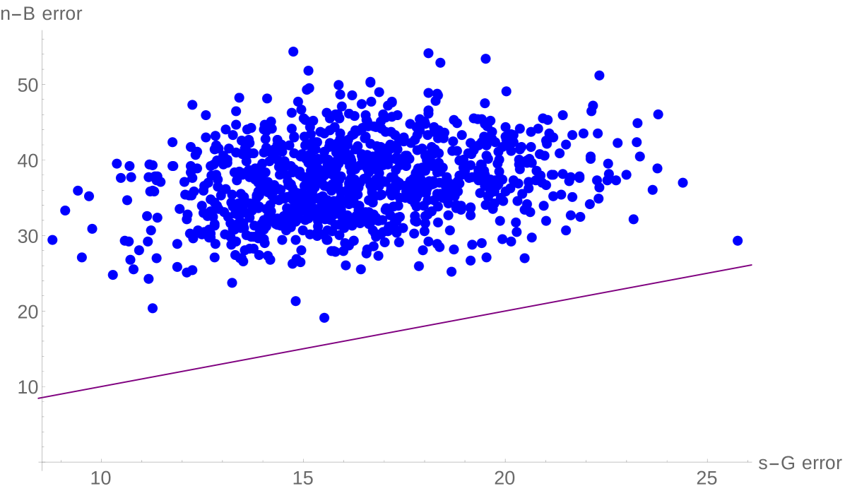
We plot the same data for matrices (again with integer coefficients from ) in Figures 5 and 6. We see that for the larger matrices, the separation between the estimates and the actual eigenvalue grows, but does much better than . In particular, out of 1000 samples, beats every time.
5.3 Domain of positive definiteness
One other way to view the problem of positive definiteness is as follows. Let us imagine that a matrix is given where the off-diagonal entries are prescribed, but the diagonal entries are free. We could then ask what condition on the diagonal entries guarantees that the matrix be positive definite?
First note that as we send the diagonal entries to infinity, the matrix is guaranteed positive definite, simply because of the Gershgorin result: as long as for all , then the matrix is positive definite. Thus we obtain at worst an unbounded box from unshifted Gershgorin.
From the fact that the shifted Gershgorin estimates are always piecewise linear, we would expect that the region from this is always an “infinite polytope”, i.e. an unbounded intersection of finitely many half-planes that is a superset of the unshifted Gershgorin box. We prove this here.
Proposition 5.2.
Let be a vector of length , and let be the set of all matrices with as the off-diagonal terms (ordered in the obvious manner). Let us define as the subset of where if , and let to be the set of all diagonals of matrices in . Then the set is an unbounded domain defined by the intersection of finitely many half-planes that contains a box of the form , and as such can be written where the entries of are nonnegative.
Proof.
We have from Theorem 3.1 that
This means that iff there exists such that for all . This is the same as saying that
Under the condition that (or under no additional condition if is odd), this is the same as
This reduces to the two conditions
which is clearly the intersection of half-planes in . Fixing the off-diagonal elements of fixes , and then is the minimum of functions linear in the diagonal elements of . Finally we know that , so that any matrix satisfying is clearly in . ∎
It follows from this proposition that shifted Gershgorin cannot be optimal. The boundary of the set must be defined by an th degree polynomial in the , since this boundary is given by an eigenvalue passing through zero and thus must be a subset of .
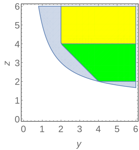
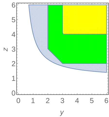
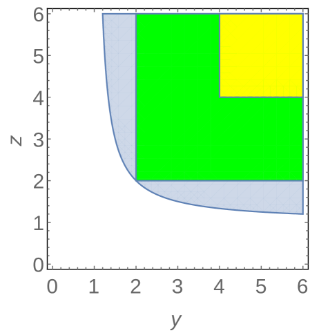
Example 5.3.
Let us consider a example for this region, and to make regions easier to plot let us only let two of the diagonal entries vary, namely
| (13) |
where are fixed parameters and are variable. From Proposition 5.2, the domain is an intersection of half-planes; the domain is given by a box, and of course the domain is given by a quadratic equation in .
Let us consider one example: choose , which is shown by the second frame in Figure 7. We can compute the conditions on as follows. We have
and the domain is defined by . Writing all of this out, we obtain the conditions
Note that unshifted Gershgorin would give the conditions . The exact boundary condition from the determinant is . We plot all of these sets in Figure 7 for this and other choices of parameters. Note that the shifted region sometimes shares boundary with the exact region, but being piecewise linear this is the best that can be done.
5.4 Spread of the off-diagonal terms
We might ask the question, given the , what are the best and worst choices of off-diagonal entries for the bound . Intuitively, it seems clear that concentrating all of the mass in a single off-diagonal element is “worst”, whereas spreading it as much as possible is “best”. In short, high off-diagonal variance is bad for the shifted estimates.
Proposition 5.4.
Let be the set of all vectors of length with nonnegative entries that sum to . We can then consider the quantities
Then and is attained at any with more than half of the entries equal to zero, and and is attained at the vector whose entries are equal to .
Proof.
The claim about is straightforward. If more than half of the entries are zero, then it is easy to see that the function is decreasing in and its supremum is attained at , giving zero. Moreover, this infimum cannot be less than zero.
For , we first show that for any with ,
First note that if all then equality is satisfied. Assume that is not a constant vector. If then the inequality is trivial, so assume . Since the average of the entries of is , at least one . Writing , we have and again the inequality follows. Finally, note that since the quantity is linear away from the points , we have
and we are done. ∎
This proposition verifies the intuition that “spreading” the mass in the off-diagonal terms improves the shifted Gershgorin bound while not changing the unshifted Gershgorin bound at all. For example, let us consider all symmetric matrices with nonnegative coefficients with all diagonal entries equal to and all off-diagonal sums equal to . Then for any in this class, . However, can be as large as if all of the off-diagonal entries are the same. Moreover, it is not hard to see that if the off-diagonal entries differ by no more than , then . In this sense, spreading the off-diagonal mass as evenly as possible helps the shifted Gershgorin bound.
Conversely, concentrating the off-diagonal mass makes the shifted Gershgorin bound worse, and, for example, if we consider the case where each row has one entry equal to and the rest zero, then . Moreover, note that this bound cannot be improved without further information, since it is sharp for where is any permutation matrix with a two-cycle.
6 Conclusions
We have shown a few cases where shifting the entries of a matrix leads to better bounds on the spectrum of the matrix. We can think of these results as a flip of the standard Perron–Frobenius theorem; the method of this paper gives good bounds on the lowest eigenvalue of a positive matrix rather than the largest.
We might ask whether the results considered here are optimal, in the sense of obtaining a spectral bound from a linear program in terms of the entries of a matrix. Of course the last condition is necessary: writing down the characteristic polynomial of a matrix and solving it gives excellent bounds on the eigenvalues, but this is a notoriously challenging approach. Most of the existing methods mentioned above (again see [2] for a comprehensive review) use some function of the off-diagonal terms, e.g. their sum, or their sum minus one distinguished element, or perhaps two subsums of the entries. This is true of all of the methods mentioned above, as is typical of results of this type. The shifted Gershgorin method uses the actual off-diagonal entries, and as we have shown above, its efficacy is a function as much of the variance of these off-diagonal terms as their sum. As we showed numerically in Section 5.2, shifted Gershgorin beats even a nonlinear method very often in a large family of matrices (to be fair, it was a family designed to work well with shifted Gershgorin, but in that class it works very well). Although checking against every existing method is beyond the scope of this paper, it seems likely that one can construct examples where shifted Gershgorin beats any existing method that uses less information about the off-diagonal terms than their actual values.
We also might ask whether this technique can be improved by shifting by a matrix other than (cf. [10] for a similar perspective on a more complicated bounding problem). Of course, if we choose any positive semidefinite matrix , write , and optimize to obtain the best bounds on the matrix , this will also give estimates on the eigenvalues of . It surely is true that for a given matrix , there could be a choice of that does better than in this regard by exploiting some feature of the original matrix . It seems unlikely that there could be a matrix that generally beats , especially in light of the results of Section 5.4. Also, there would be the challenge of knowing was positive semi-definite in the first place: it seems unlikely that one could bootstrap this method by writing , since this would give , and one is still optimizing over multiples of . However, if there is some known structure of that matches the structure of a known semi-definite (e.g. is a covariance matrix or more generally a Gram matrix) then this might allow us to obtain tighter bounds on the spectrum of .
Acknowledgments
The author would like to thank Jared Bronski for useful discussions.
References
- [1] S. A. Gershgorin. Uber die Abgrenzung der Eigenwerte einer Matrix. Bulletin of the Russian Academy of Sciences, (6):749–7–54, 1931.
- [2] Richard S. Varga. Gershgorin and his circles in springer series in computational mathematics, 36, 2004.
- [3] Alexander Ostrowski. Über die Determinanten mit überwiegender Hauptdiagonale. Commentarii Mathematici Helvetici, 10(1):69—96, 1937.
- [4] Alfred Brauer. Limits for the characteristic roots of a matrix. ii. Duke Math. J., 14(1):21–26, 03 1947.
- [5] Aaron Melman. Generalizations of Gershgorin disks and polynomial zeros. Proceedings of the American Mathematical Society, 138(7):2349—2364, 2010.
- [6] Ljiljana Cvetkovic, Vladimir Kostic, and Richard S. Varga. A new Geršgorin-type eigenvalue inclusion set. Electronic Transactions on Numerical Analysis, 18:73—80, 2004.
- [7] Roger A Horn and Charles R Johnson. Topics in matrix analysis. Cambridge Univ. Press Cambridge etc, 1991.
- [8] Richard Courant and David Hilbert. Methods of mathematical physics, volume 1. CUP Archive, 1966.
- [9] Oliver Riordan and Alex Selby. The maximum degree of a random graph. Combinatorics, Probability and Computing, 9(06):549–572, 2000.
- [10] Nicholas J Higham and Françoise Tisseur. Bounds for eigenvalues of matrix polynomials. Linear algebra and its applications, 358(1):5–22, 2003.