Optimizing stakes in simultaneous bets
Abstract.
We want to find the convex combination of iid Bernoulli random variables that maximizes for a given threshold . Endre Csóka conjectured that such an is an average if , where is the success probability of the Bernoulli random variables. We prove this conjecture for a range of and .
Key words and phrases:
bold play, intersecting family, stochastic inequality, tail probability.2010 Mathematics Subject Classification:
60G50, 05D05We study tail probabilities of convex combinations of iid Bernoulli random variables. More specifically, let be an infinite sequence of independent Bernoulli random variables with success probability , and let be a real number. We consider the problem of maximizing over all sequences of non-negative reals such that . By the weak law of large numbers, the supremum of is equal to if . That is why we restrict our attention to .
As a motivating example, consider a venture capitalist who has a certain fortune to invest in any number of startup companies. Each startup has an (independent) probability of succeeding, in which case it yields a return on investment. If the capitalist divides his fortune into a (possibly infinite!) sequence of investments, then his total return is . Suppose he wants to maximize the probability that the total return reaches a threshold . Then we get our problem with .
The problem has a how-to-gamble-if-you-must flavor [6]: the capitalist places stakes on a sequence of simultaneous bets. There is no need to place stakes higher than . The way to go all out, i.e., bold play, is to stake on bets, but this is not a convex combination. That is why we say that staking on bets with is bold play.
In a convex combination we order . We denote the sequence by and write . We study the function
| (1) |
for . It is non-decreasing in and non-increasing in . The following has been conjectured by Csóka [5], who was inspired by some well known open problems in combinatorics:
Conjecture 1 (Csóka).
For every and there exists a such that is realized by if and if for some . In other words, the maximal probability is realized by an average.
If the conjecture is true, then is a binomial tail probability and we still need to determine the optimal . Numerical results of Csóka suggest that bold play is optimal for most parameter values.
We are able to settle the conjecture for certain parameter values, as illustrated in figure 1 below.
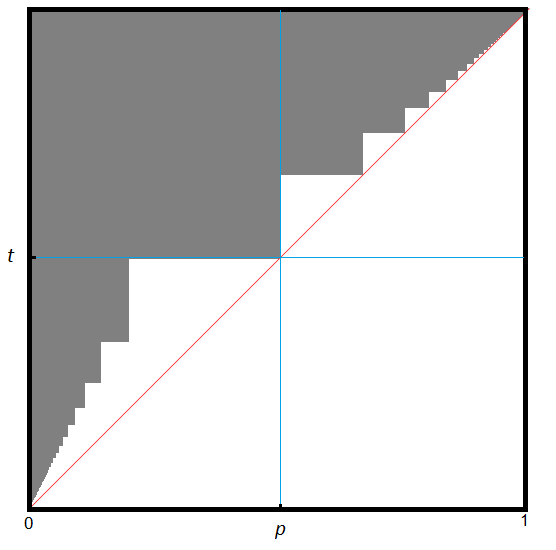
It is natural to expect, though we are unable to prove this, that a gambler becomes bolder if the threshold goes up or if the odds go down. In particular, if and and if bold play is optimal for , then it is natural to expect that bold play is optimal for as well. This is clearly visible in the figure above, which is a union of rectangles with lower right vertices and for .
Our paper is organized as follows. We first lay the groundwork by analyzing properties of and prove that the supremum in equation 1 is a maximum. Then we cover the shaded region in figure 1 for the three separate parts of odds greater than one, threshold greater than half, and odds smaller than one. Finally, we recall an old result on binomial probabilities which would imply that (assuming Csóka’s conjecture holds and bold play is stable in the sense that we just explained) bold play is optimal if for all .
1. Related problems and results
According to Csóka’s conjecture, if the coin is fixed and the stakes vary, then the maximum tail probability is attained by a (scaled) binomial. If the stake is fixed and the coins vary, then Chebyshev already showed that the maximum probability is attained by a binomial:
Theorem 2 (Chebyshev, [21]).
For a given and , let be any sum of independent Bernoullis such that . Then is maximized by Bernoullis for which the success probabilities assume at most three different values, only one of which is distinct from and . In particular, the maximum is a binomial tail probability.
Samuels considered a more general situation with fixed expectations and arbitrary random variables.
Conjecture 3 (Samuels, [20]).
Let be such that . Consider over all collections of independent non-negative random variables such that . This supremum is a maximum which is attained by for and for , where is an integer, the are Bernoulli random variables, and . In other words, the gambler accumulates from small expectations before switching to bold play.
If all are equal, then the are identically distributed, and the conjecture predicts that the maximum probability is attained by a binomial.
If one assumes that the Samuels conjecture holds, then one still needs to determine the optimal . If then the optimal is equal to zero [1]. This implies that another well-known conjecture is a consequence of Samuels’ conjecture, see also [18].
Conjecture 4 (Feige, [7]).
For all collections of independent non-negative random variables such that it is true that
As a step towards solving this conjecture, Feige proved the remarkable theorem that there exists a such that . His original value of has been gradually improved. The current best result is by Guo et al [12].
2. Properties of
The function is defined on a region bounded by a rectangular triangle. It is easy to compute its value on the legs of the triangle: and . It is much harder to compute the value on the hypothenuse.
Proposition 5.
if .
Proof.
We follow the proof of [2, Lemma 1]. The following Paley-Zygmund type inequality for random variables of zero mean was proved in [13, lemma 2.2] and extended in [14]:
Applying this to we have
The second moment of is equal to and the fourth moment is equal to
This can be bounded by
The Paley-Zygmund type inequality produces a lower bound on . Its complementary probability is bounded by:
It is possible to improve on this bound for small by using Feige’s theorem. We write . Then . Note that and we write . We can approximate this probability by a truncated sum , where is a sum of independent random variables of expectation . By dividing by and applying the bound of [12] we find
We have two upper bounds. The first is more restrictive for large and the second is more restrictive for small . The lower bound follows from bold play. Let be such that . If is the average of Bernoullis, then . This is minimal and equal to if . ∎
We say that a sequence is finite if for all but finitely many , and infinite otherwise.
Proposition 6.
Proof.
According to Jessen and Wintner’s law of pure type [3, Theorem 3.5], either for each or there exists a countable set such that . In other words, the random variable is either non-atomic or discrete. If and are independent, and if is non-atomic, then the convolution formula implies that is non-atomic.
Suppose that is infinite. We prove that is non-atomic. Let be a subsequence such that . Let be the set of all and let be its complement. Then both and are either discrete or non-atomic. By our choice of , has the property that its value determines the values of all for . This implies that is non-atomic. Therefore, is non-atomic. In particular .
Denote a truncated sum by . By monotonic convergence . Therefore, for any infinite , can be approximated by tail probabilities of finite convex combinations. ∎
Csóka conjectures that the tail probability is maximized by an average. This would imply that the sup in proposition 6 is a max. We are unable to prove this, but we can prove that the sup in equation 1 is a max.
Theorem 7.
If then for some . Furthermore, is left-continuous in .
Proof.
We write . Since is decreasing in , it suffices to show that there exists an such that . Let be such that converges to for an increasing sequence . By a standard diagonal argument we can assume that is convergent for all . Let and let . Then is a non-increasing sequence which adds up to . Observe that cannot be the all zero sequence, since this would imply that and , so converges to in distribution. Since we limit ourselves to , this means that which is nonsense. Therefore, .
We first prove that . Fix an arbitrary . Let be such that and . Let be such that and for all . Now
so by our assumptions
where we write . Observe that
and
By Chebyshev’s inequality, we conclude that for sufficiently small . It follows that
By taking limits and we conclude that
Let . Then is a convex combination such that
Therefore, and these inequalities are equalities. ∎
We now more or less repeat this proof to show that is continuous in . Since we need to vary , we write for a Bernoulli with succes probability and .
Theorem 8.
is continuous in .
Proof.
For any choose a finite such that . If converges to then converges to in probability. Since is finite
It follows that for any sequence . Since is increasing in , it follows that is left-continuous in .
We need to prove right continuity, i.e., . This is trivially true on the hypothenuse, because this is the right-hand boundary of the domain. Consider . Let and be such that . By a standard diagonal argument we can assume that converges coordinatewise to some , which may not sum up to one. It cannot be the all zero sequence, i.e., the sum is not zero, by the same argument as in the proof of theorem 7. The sequence therefore sums up to for some . Again, we split where and . We choose such that and . Similarly, where converges to in probability, and for sufficiently large . As in the previous proof, Chebyshev’s inequality and convergence in probability imply
for sufficiently large . By taking limits and it follows that . If we standardize to a sequence so that we get a convex combination, we again find that . ∎
3. Favorable odds
We consider . In this case, bold play comes down to a single stake . We say that is an interval of length if for some , which we call the initial element. We say that two intervals and are separate if is not an interval. If is a family of sets, then we write for the union of all these sets.
Lemma 9.
Let be a family of intervals of length in such that is a proper subset. Then .
Proof.
is a union of say separate intervals, all of lengths . Any interval of length contains intervals of length . Therefore, contains intervals of length . It follows that . ∎
Two families and are cross-intersecting if for all and .
Lemma 10.
Let be a family of intervals of length in . Let be a family of intervals of length such and are cross-intersecting. Then .
Proof.
Let be any element in . An interval intersects if and only if , which is an interval of length . Therefore, the set of initial elements of intervals in is contained in an intersection of intervals of length . The complement of thus contains a union of intervals of length . By the previous lemma, this union has cardinality . Therefore, contains at most elements. ∎
Lemma 11.
Let be a finite measure space such that and let for be such that . Then .
Proof.
∎
Theorem 12.
If for some positive integer , then bold play is optimal.
Proof.
Bold play gives a probability of reaching . We need to prove that for arbitrary . By proposition 6 we may assume that is finite. It suffices to prove that for rational , since is monotonic in .
Let be the number of non-zero in and let . Let be a sequence of independent discrete uniform random variables, i.e, for with probability . Let for . Then and are identically distributed. Think of as an assignment of weight to a random element in . Let be the sum of the coefficients – the load – that is assigned to . Then , i.e., is the load of . Instead of we might as well select any interval . If is the load of , then , and . We need to prove that .
Let be the sample space of the . For , let be the cardinality of . In particular, . It suffices to prove that . Assume that for some . Apply lemma 11 to the counting measure to find
Note that if and only if has load . Therefore, there are at least elements such that the intervals all have load . The intersection of these intervals is equal to
It has load by lemma 11. Its complement has load . If then has load and therefore it intersects for all . There are such intervals , and we denote this family by . Let be the family of with . Lemma 10 applies since the length of is and since . We conclude that . ∎
With some additional effort, we can push this result to the hypothenuse.
Proposition 13.
If for some positive integer , then bold play is optimal if , and is optimal if .
Proof.
By proposition 6 it suffices to prove that for finite . We adopt the notation of the previous theorem. Let be the number of non-zero coefficients in , and let be random selections of . We assign the coefficients according to these selections and let be the load of the set . Each is identically distributed to . For let be the number of that reach the threshold, or equivalently, the number of loads . We have . In the proof above, we showed that if . This is no longer true now that we have . It may happen that in which case all are equal to and all loads are equal to . Note that this can only happen if all are bounded by , so .
We think of the coefficients as being assigned one by one in increasing order. In particular, and are placed last. If , then either or of the loads are equal to before and are placed. In the first case, there are two remaining loads and the probability that are are placed here is . In the second case, there is only one remaining load and the probability that and are placed here is . We conclude that and therefore
is bounded by . Thus we obtain . This bound is reached if and .
Let and let . We first consider the case that . suppose there are two remaining loads before and are placed, then each and can only be assigned to a unique place to complete all loads to . Since , there are at least two loads before the final two coefficients are placed. Let assign for in the same way as , but it reassigns to and to . Then , because the loads at and exceed the threshold. We can reconstruct from because the loads at and are the only ones that exceed the threshold for , and their values are different because . We have a correspondence between and . Let and let . Then and . This implies that
In particular and bold play is optimal.
Finally, consider the remaining case and and . In this case, we may switch the assignments of and to complete the loads. Let represent this switch (it may be equal to if the assignments are the same). Again, let and be two locations for which the loads have already been completed before and are placed. Let be the elements which assign the first coefficients in the same way, but assigns the final two elements to and . In particular, . We can reconstruct from , the correspondence is injective, so again and we conclude in the same way that bold play is optimal. ∎
If bold play is stable, as discussed above, then proposition 13 would imply that bold play is optimal if for . Establishing this stability of bold play appears to be hard, and we are able to settle only one specific case in the range .
Proposition 14.
If and , then bold play is optimal if .
Proof.
We randomly distribute the coefficients of a finite over locations. Let be the load of the discrete interval , where as before we reduce modulo . Then and the sum of all is equal to . Let be the number of that reach the threshold. Not all can reach the threshold and therefore . Then
We need to prove that . If then we are done. Therefore, we may assume that . Only one of the does not meet the threshold and without loss of generality we may assume it is , which has load . The other reach the threshold, and since the sum of all is equal to , we find that
In other words, . If then does not reach the threshold if it does not include . Only of the include , contradicting our assumption that . Therefore and since the same applies to we have in fact that . Since we have that all other than . In particular, . We find that and . The sum of the remaining , with is at least and the sum of all is . Since all the remaining have to be equal to . It follows that the loads alternate between zero and : if is odd and if is even. We conclude that if then all non-zero loads are equal and only two non-zero loads are consecutive. There are exactly such arrangements. There are also arrangements in which the non-zero loads are consecutive. In this case . It follows that , which implies that . Bold play is optimal. ∎
These results conclude our analysis of the upper right hand block of figure 1. A zigzag of triangles along the hypothenuse remains. Numerical results of Csóka [5] suggest that bold play is optimal for all of these triangles, except for the one touching on . In the next section we will confirm that bold play is not optimal for this triangle.
4. High threshold
We now consider the case , when bold play comes down to a single stake . We need to maximize and we may assume that is finite by proposition 6. Suppose that has non-zero coefficients, i.e., . Let be the family of , such that . Let . Then
| (2) |
Therefore we need to determine the family that maximizes the sum on the right hand side. Problems of this type are studied in extremal combinatorics, see [8] for recent progress. A family is intersecting if no two elements are disjoint. Two standard examples of intersecting families are , the family of all such that , and , the family of all subsets such that . Fishburn et al [9] settled the problem of maximizing
over all intersecting families :
Theorem 15 (Fishburn et al).
For a fixed , let be any intersecting family of subsets from . If then is maximized by . If and is odd, then is maximized by .
Proof.
Following [9]. First suppose is odd. At most one of and can be in . If , then if . Therefore is maximal if contains each set of largest cardinality. It follows that maximizes if is odd and .
Now consider an arbitrary and . Let be the cardinality of the subfamily At most one of and can be in and therefore . Since we have if . For we want to maximize under the constraint (for it does not matter which of the two subsets we select, as long as we select one of them). By the Erdős-Ko-Rado theorem, if then is maximized by a family of subsets that contain one common element. For such a family, . It follows that is maximal if . ∎
Note that corresponds to if and , i.e., bold play.
Corollary 16.
If then bold play is optimal.
Proof.
If then is intersecting. The maximizing family corresponds to with . This takes care of the upper left-hand block in figure 1. ∎
The positive odds part of theorem 15 can be applied to the triangle touching on that we mentioned above. The family can be represented by if and , by taking .
Corollary 17.
If then bold play is not optimal.
Proof.
Choose maximal such that and set . Then is the unique maximizer of and corresponds to , which is not bold play. ∎
Finally, we settle the remaining part of the box in the upper left corner of figure 1.
Corollary 18.
If then bold play is optimal.
Proof.
Note that we may restrict our attention to such that and that bold play corresponds to .
If then by theorem 15. We find that with equality for bold play. ∎
These results take care of the box in the upper left corner of figure 1, including its boundaries.
5. Unfavorable odds
A family has matching number , denoted by , if the maximum number of pairwise disjoint is equal to . In particular, is intersecting if and only if . The matching number of is bounded by , because for each and sums up to one.
A family is -uniform if all its elements have cardinality . According to the Erdős matching conjecture [1, 10, 11], if then the maximum cardinality of a -uniform family such that is either attained by , the family of all -subsets containing at least one element from , or by , the family containing all -subsets from . Frankl [10] proved that has maximum cardinality if . For recent progress on this conjecture, see [11] and the references therein.
Theorem 19.
If and for some positive integer then bold play is optimal.
Proof.
We need to prove that for finite . For a large enough we have that if . We have
where denotes the number of subsets of cardinality . By Frankl’s result, we can put a bound on if . For larger we simply bound by . In this way we get that is bounded by
which is equal to
for . By our assumptions, there exists a such that . If then since . ∎
We can push this result to the hypothenuse, using the same approach as in the proof of proposition 13, in one particular case: . By stability, one would expect that bold play is optimal for any but we can only prove this for for integers .
Proposition 20.
Bold play is optimal if and for an integer .
Proof.
We may assume that is finite and we randomly assign its coefficients to . We denote , the load at zero, by and we need to prove that
which is the success probability of bold play if . Let be the number of loads exceeding the threshold of before the last two coefficients and are assigned. Obviously, is either equal to or or . We will show that for .
Suppose that . In this case, if reaches the threshold, then at least one of the two final coefficients has to be placed in . This happens with probability .
Suppose that . One load has reached the threshold before the final two coefficients are placed. This load is in with probability . If the load is not in , then at least one of the remaining two coefficients has to be placed there. This happens with probability . We conclude that
Suppose that . In other words, two loads have already reached the threshold before the final two coefficients are placed. The probability that one of these two loads is in is . If none of the two loads is in , then can only reach the threshold if both remaining coefficients are assigned to . The probability that this happens is .
if . ∎
6. Binomial tails
If conjecture 1 holds, then the tail probability is maximized by a Bernoulli average and we need to determine the optimal . It is more convenient to state this in terms of binomials. For a fixed and , maximize
for a positive integer . Since the probability increases if increases and does not pass an integer, we may restrict our attention to such that for some integer . In other words, we need to only consider for . If is the reciprocal of an integer , then the are multiples of . This is a classical problem. In 1693 John Smith asked which is optimal if and . Or in his original words, which of the following events is most likely: fling at least one six with 6 dice, or at least two sixes with 12 dice, or at least three sixes with 18 dice. The problem was communicated by Samuel Pepys to Isaac Newton, who computed the probabilities. Chaundy and Bullard [4] gave a very nice historical description (more history can be found in [16, 17]) and solved the problem, see also [15].
Theorem 21 (Chaundy and Bullard).
For an integer , is maximal for . Even more so, the tail probabilities strictly decrease with .
In other words, if and if Csóka’s conjecture holds, then bold play is optimal. By stability, one would expect that bold play is optimal for . It turns out that it is possible to extend Chaundy and Bullard’s theorem in this direction and prove that decreases with for arbitrary , see [19, Theorem 1.5.4].
7. Conclusion
We settled Csóka’s conjecture for a range of parameters building on combinatorial methods. Csóka’s conjecture predicts that attains its maximum at an extreme point of the subset of positive non-increasing sequences in the unit ball in . Perhaps variational methods need to be considered.
Christos Pelekis was supported by the Czech Science Foundation (GAČR project 18-01472Y), by the Czech Academy of Sciences (RVO: 67985840), and by a visitor grant of the Dutch mathematics cluster Diamant.
References
- [1] N. Alon, P. Frankl, H. Huang, V. Rödl, A. Ruciński, B. Sudakov, Large matchings in uniform hypergraphs and the conjectures of Erdős and Samuels. J. Combin. Th., Ser. A 119 (2012) 1200–1215.
- [2] I. Arieli, Y. Babichenko, R. Peretz, H. Peyton Young, The speed of innovation in social networks. Econometrica 88 no. 2 (2020), 569–594.
- [3] L. Breiman, Probability, Reading, Addison-Wesley, 1968.
- [4] T.W. Chaundy, J.E. Bullard, John Smith’s problem. Math. Gazette 44(350), (1960), 253–260.
- [5] E. Csóka, Limit theory of discrete mathematics problems. arXiv1505.06984.
- [6] L. E. Dubins and L. J. Savage, Inequalities for Stochastic Processes (How to Gamble If You Must). Dover, 1976.
- [7] U. Feige, On sums of independent random variables with unbounded variances, and estimating the average degree in a graph. SIAM J. Comput. 35 (2006), 964–984.
- [8] Y. Filmus, The weighted complete intersection theorem. J. Combin. Th. Ser. A 151 (2017), 84–101.
- [9] P.C. Fishburn, P. Frankl, D. Freed, J. Lagarias, A.M. Odlyzko. Probabilities for intersecting systems and random subsets of finite sets. SIAM. J. Algebraic Discrete Methods 7 no. 1 (1986) 73–79.
- [10] P. Frankl, Improved bounds on Erdős’ matching conjecture. J. Combin. Th., ser. A, 120 (2013) 1068–1072.
- [11] P. Frankl, A. Kupavskii, Some results around the Erdős matching conjecture. Acta Math. Univ. Comenianae 88 no. 3 (2019), 695–699.
- [12] J. Guo, S. He, Z. Ling, Y. Liu, Bounding probability of small deviation on sum of independent random variables: Combination of moment approach and Berry-Esseen theorem. arXiv:2003.03197.
- [13] S. He, Z. Q. Luo, J. Nie, S. Zhang, Semidefinite relaxation bounds for indefinite homogeneous quadratic optimization. SIAM J. Optim. 19 (2007) 503–523.
- [14] S. He, J. Zhang, S. Zhang, Bounding probability of small deviation: a fourth moment approach. Math. Oper. Res. 45 no. 1 (2010), 208–232.
- [15] K. Jogdeo, S.M. Samuels, Monotone Convergence of Binomial Probabilities and a Generalization of Ramanujan’s Equation. Ann. Math. Statist. 39 no. 4, (1968), 1191–1195.
- [16] T.H. Koornwinder, M.J. Schlosser, On an identity by Chaundy and Bullard, I. Indag. Math. (NS) 19, (2008), 239–261.
- [17] T.H. Koornwinder, M.J. Schlosser, On an identity by Chaundy and Bullard, II. Indag. Math. (NS) 24, (2013), 174–180.
- [18] R. Paulin, On some conjectures by Feige and Samuels. arXiv1703.05152.
- [19] C. Pelekis, Search games on hypergraphs. PhD thesis, TU Delft, 2014.
- [20] S.M. Samuels, On a Chebyshev-type inequality for sums of independent random variables. Ann. Math. Statist. 37 no. 1, (1966), 248–259.
- [21] P. Tchebichef, Démonstration élémentaire d’une proposition générale de la theorie des probabilités. J. Reine. Angew. Math. 33 (1848), 259–267.
Institute of Applied Mathematics
Delft University of Technology
Mourikbroekmanweg 6
2628 XE Delft, The Netherlands
r.j.fokkink@tudelft.nl, l.e.meester@tudelft.nl
School of Electrical and Computer Engineering
National Technical University of Athens
Zografou, 15780, Greece
pelekis.chr@gmail.com