Optional games on cycles and complete graphs

Hyeong-Chai Jeong¹¹1E-mail:hcj@sejong.ac.kr Seung-Yoon Oh Benjamin Allen Martin A. Nowak Department of Physics, Sejong University, Gangjingu, Seoul 143-747, KOREA Program for Evolutionary Dynamics, Harvard University,Cambridge, MA 20138, USA Department of Mathematics, Emmanuel College, Boston, MA 02115 USA; Department of Mathematics, Harvard University,Cambridge, MA 20138, USA Department of Organismic and Evolutionary Biology, Harvard University,Cambridge, MA 20138, USA

Abstract

We study stochastic evolution of optional games on simple graphs. There are two strategies, A and B, whose interaction is described by a general payoff matrix. In addition there are one or several possibilities to opt out from the game by adopting loner strategies. Optional games lead to relaxed social dilemmas. Here we explore the interaction between spatial structure and optional games. We find that increasing the number of loner strategies (or equivalently increasing mutational bias toward loner strategies) facilitates evolution of cooperation both in well-mixed and in structured populations. We derive various limits for weak selection and large population size. For some cases we derive analytic results for strong selection. We also analyze strategy selection numerically for finite selection intensity and discuss combined effects of optionality and spatial structure.

keywords: Evolutionary game theory, Evolutionary graph theory, Evolution of cooperation, Spatial games

1 Introduction

In the typical setting of evolutionary game theory, the individual has to adopt one of several strategies (Hofbauer & Sigmund,, 1988; Weibull,, 1997; Friedman,, 1998; Hofbauer & Sigmund,, 1998; Cressman,, 2003; Nowak,, 2004; Vincent & Brown,, 2005; Gokhale & Traulsen,, 2011). For example in a standard cooperative dilemma (Hauert et al.,, 2006; Nowak,, 2012; Rand & Nowak,, 2013; Hauert et al.,, 2014), the individual can choose between cooperation and defection. Natural selection tends to oppose cooperation unless a mechanism for evolution of cooperation is at work (Nowak, 2006a, ). In optional games there is also the possibility not to play the game (Kitcher,, 1993; Batali & Kitcher,, 1995; Hauert et al.,, 2002; Hauert,, 2002; Szabó & Hauert, 2002a, ; De Silva et al.,, 2009; Rand & Nowak,, 2011). The individual player has to choose whether to participate in the game (by cooperating or defecting) or to opt out. Opting out leads to fixed “loner’s payoff”. This loner’s payoff is forfeited if one decides to play the game. Thus there is a cost for playing the game. Optional games tend to lead to relaxed social dilemmas (Michor & Nowak,, 2002; Hauert et al.,, 2006). They have also been used to study the effect of costly punishment (by peers and institutions) on evolution of cooperation (Boyd & Richerson,, 1992; Nakamaru & Iwasa,, 2005; Hauert et al.,, 2007; Sigmund,, 2007; Traulsen et al.,, 2009; Hilbe & Sigmund,, 2010). There is also a relationship between optional games and empty places in spatial settings (Nowak et al.,, 1994).

Here we study the effect of optional games on cycles and on complete graphs (van Veelen & Nowak,, 2012). Cycles and complete graphs are on opposite ends of the spectrum of spatial structure. Most graphs will lead to an evolutionary dynamics between these two extremes. Evolutionary graph theory (Lieberman et al.,, 2005; Santos & Pacheco,, 2005; Ohtsuki et al.,, 2006; Szabó & Fáth,, 2007; Fu et al., 2007a, ; Fu et al., 2007b, ; Santos et al.,, 2008; Perc & Szolnoki,, 2010; Perc,, 2011; Allen et al.,, 2013; Maciejewski,, 2014; Allen & Nowak,, 2014) is an approach to study the effect of population structure on evolutionary dynamics (Nowak & May,, 1992; Nakamaru et al.,, 1997; Tarnita et al., 2009b, ; Tarnita et al., 2009a, ; Nowak et al.,, 2010; Tarnita et al.,, 2011). Using stochastic evolutionary dynamics for games in finite populations (Foster & Young,, 1990; Challet & Zhang,, 1997; Taylor et al.,, 2004; Nowak et al.,, 2004; Imhof & Nowak,, 2006; Traulsen et al.,, 2006), we notice that the number of different loner strategies has an important effect on selection between strategies that occur in the game. Increasing the number of ways to opt out (or, increasing mutational bias toward (Garcia & Traulsen,, 2012) loner strategies) in general favors evolution of cooperation.

Our paper is organized as follows. In Section 2 we give an overview of the basic model and list our key results. In Section 3 we calculate abundance in the low mutation limit. It is used to investigate the conditions for strategy selection in the weak selection limit in Section 4 and in the strong selection limit in Section 5. We calculate these conditions for optional games with simplified prisoner’s dilemma games in Section 6. We then analyze strategy selection numerically for finite mutation rate as well as finite selection intensity in low mutation in Section 7. In our concluding remarks in Section 8, we summarize and discuss the implications of our findings.

2 Model and main results

We consider stochastic evolutionary dynamics of populations on graphs. In particular, we investigate the condition for one strategy to be favored over the others in the limit of low mutation and for two different reproduction processes, birth-death (BD) updating and death-birth (DB) updating on cycles. We compare the results with those for the Moran Process (MP) on the complete graph. The fitness of an individual is determined by the payoff from the non-repeated matrix games with its nearest neighbors. We use exponential fitness,

\displaystyle f_{r}

\displaystyle=

\displaystyle e^{wP_{r}},

(1)

for the individual at the site $r$ , where $P_{r}$ is its accumulated payoff from the games with its neighbors. The intensity of selection, $w$ , is a parameter representing how strongly the fitness of an individual depends on the its payoff.

We first study a general matrix game whose payoff matrix is given by $A=[\,a_{ij}\,]$ , i.e., a game that an individual using strategy $S_{i}$ receives $a_{ij}$ as a payoff when it plays with an individual with strategy $S_{j}$ . Then we apply our finding to an optional prisoner’s dilemma game to find a condition for evolution of cooperation.

We calculate abundance (frequencies in the stationary distribution) of strategies in the low mutation limit, where mutation rate $u$ goes to zero, and find the condition that strategy $S_{i}$ is more abundant than strategy $S_{j}$ . For low mutation, abundance can be written in terms of fixation probabilities which we obtain in a closed form for general $w$ . Although the formal expression of abundance is useful for numerical calculation, the complexity of the expression makes it hard for us to understand the strategy selection mechanism intuitively.

For low intensity of selection ( $w\rightarrow 0$ ), however, the fixation probability reduces to a linear expression in $a_{ij}$ with clear interpretation. The condition for strategy selection is then given by a simple linear inequality in terms of payoff matrix elements. This is the case even for the large population limit of $N\rightarrow\infty$ .

However, when considering the limits of weak selection ( $w\to 0$ ) and large population ( $N\to\infty$ ), the condition for strategy selection depends on the order in which these limits are taken. We therefore consider two different large population, weak selection limits: the $wN$ limit and the $Nw$ imit. In the $wN$ limit, $w$ goes to zero before $N$ goes to infinity such that $Nw$ is much smaller than 1. In the $Nw$ limit, $N$ goes to infinity before $w$ goes to zero such that $Nw$ is much larger than 1.

2.1 $wN$ limit

We first calculate the fixation probability, $\rho_{ik}$ , which is the probability that a singe $S_{i}$ takes over the whole population of the strategy $S_{k}$ for the $w\rightarrow 0$ limit. It can be written as

\displaystyle\rho_{ik}

\displaystyle=

\displaystyle\frac{1}{N}+d_{ik}\,w.

(2)

Here, the “biased drift”, $d_{ik}$ is defined by

\displaystyle\mbox{}\hskip-5.69054ptd_{ik}

\displaystyle=

\displaystyle\left\{\begin{array}[]{ll}\frac{1}{2}\,l_{ik}-\frac{1}{2N}\,s_{ik}&\mbox{}\hskip-5.69054pt\mbox{}\hskip-5.69054pt\hskip 14.22636pt\mbox{for}\ \ \mbox{BD}\\ \frac{1}{4}\,l_{ik}-\frac{1}{4N}\,s_{ik}&\mbox{}\hskip-5.69054pt\mbox{}\hskip-5.69054pt\hskip 14.22636pt\mbox{for}\ \ \mbox{DB}\\ \frac{1}{4}\,l_{ik}-\frac{1}{12}\,s_{ik}&\mbox{}\hskip-5.69054pt\mbox{}\hskip-5.69054pt\hskip 14.22636pt\mbox{for}\ \ \mbox{MP}\end{array}\right.

(6)

with the anti-symmetric term $l_{ik}$ and the symmetric term $s_{ik}$ given by

	$\displaystyle l_{ik}$	$\displaystyle=$	$\displaystyle\sigma_{\!{}_{N}}a_{ii}+a_{ik}-a_{ki}-\sigma_{\!{}_{N}}a_{kk}$
	$\displaystyle s_{ik}$	$\displaystyle=$	$\displaystyle\sigma_{\!{}_{N}}\left({a_{ii}-a_{ik}-a_{ki}+a_{kk}}\right).$		(7)

The structure factor, $\sigma_{\!{}_{N}}$ for the population of the size $N$ , is given by

\displaystyle\sigma_{\!{}_{N}}

\displaystyle=

\displaystyle\left\{\begin{array}[]{ll}1-2/N&\hskip 14.22636pt\mbox{for}\ \ \mbox{BD\ \& \ MP}\\ 3-8/N&\hskip 14.22636pt\mbox{for}\ \ \mbox{DB}.\end{array}\right.

(10)

Using fixation probabilities of Eq. (2), we then calculate abundance in the low mutation limit and show that strategy $S_{i}$ is more abundant than strategy $S_{j}$ when

\displaystyle\sum_{k}\,l_{ik}

\displaystyle>

\displaystyle\sum_{k}\,l_{jk}

(11)

as previously known (Nowak et al.,, 2010; Ohtsuki & Nowak,, 2006). The fixation probability obtained for a general $2\times 2$ matrix game is also applied to calculate abundance of cooperator and defectors in optional prisoner’s dilemma game(Szabó & Hauert, 2002b, ) with $(n+2)$ strategies, cooperator (C), defector (D) and $n$ different types of loners, $L_{1},\cdots,L_{n}$ . The payoff matrix is given by

\displaystyle\hskip-28.45274pt\begin{array}[]{cl}\mbox{}&\begin{array}[]{ccccc}\mbox{}\hskip 14.22636ptC&\mbox{}\hskip 2.84526pt\ \ D&\mbox{}\hskip 2.84526pt\ \ L_{1}&\ \cdots&\ L_{n}\end{array}\\ \begin{array}[]{c}C\\ D\\ L_{1}\\ \vdots\\ L_{n}\end{array}&\left(\begin{array}[]{ccccc}\mbox{}\hskip 2.84526ptR&\mbox{}\hskip 14.22636ptS&\mbox{}\hskip 14.22636ptg&\mbox{}\hskip 2.84526pt\cdots&\mbox{}\hskip 14.22636ptg\\ \mbox{}\hskip 2.84526ptT&\mbox{}\hskip 14.22636ptP&\mbox{}\hskip 14.22636ptg&\mbox{}\hskip 2.84526pt\cdots&\mbox{}\hskip 14.22636ptg\\ \mbox{}\hskip 2.84526ptg&\mbox{}\hskip 14.22636ptg&\mbox{}\hskip 14.22636ptg&\mbox{}\hskip 2.84526pt\cdots&\mbox{}\hskip 14.22636ptg\\ \mbox{}\hskip 2.84526pt\vdots&\mbox{}\hskip 14.22636pt\vdots&\mbox{}\hskip 14.22636pt\vdots&\mbox{}\hskip 2.84526pt\ddots&\mbox{}\hskip 14.22636pt\vdots\\ \mbox{}\hskip 2.84526ptg&\mbox{}\hskip 14.22636ptg&\mbox{}\hskip 14.22636ptg&\mbox{}\hskip 2.84526pt\cdots&\mbox{}\hskip 14.22636ptg\\ \end{array}\right).\end{array}

(25)

When two cooperators meet, both get payoff $R$ . When two defectors meet, they get payoff $P$ . If a cooperator meets a defector, the defector gets the payoff $T$ while the cooperator get the payoff $S$ . Loners get payoff $g$ always. Cooperators or defectors also get payoff $g$ when they meet a loner. Since the $n$ different types of loners have the same payoff structure, this system is equivalent to to the population with three strategies, $C$ , $D$ , and a single type of loners, $L$ if the mutation rate toward $L$ (from $C$ or $D$ ) is $n$ times larger than the other way.

In the limit of $w$ goes to zero, we find that the condition for $x_{\!{}_{C}}>x_{\!{}_{D}}$ is given as

\displaystyle\sigma_{\!{}_{N}}(n)\,R+S

\displaystyle>

\displaystyle T+\sigma_{\!{}_{N}}(n)\,P,

(26)

where

\displaystyle\mbox{}\hskip-5.69054pt\mbox{}\hskip-5.69054pt\mbox{}\hskip-5.69054pt\sigma_{\!{}_{N}}(n)\mbox{}\hskip-5.69054pt

\displaystyle=

\displaystyle\mbox{}\hskip-5.69054pt\left\{\begin{array}[]{lll}\left({1+\frac{1}{2}\,n}\right)\left({1-\frac{2}{N}}\right)\mbox{}\hskip-5.69054pt&\mbox{}\hskip-5.69054pt\hskip 14.22636pt\mbox{for}\ \ \mbox{BD\ \& MP}\\ \left({1+\frac{1}{2}\,n}\right)\left({3-\frac{8}{N}}\right)\mbox{}\hskip-5.69054pt&\mbox{}\hskip-5.69054pt\hskip 14.22636pt\mbox{for}\ \ \mbox{DB}.\end{array}\right.

(29)

As long as $w$ goes to zero first ( $Nw\ll 1$ ), inequality (26) is valid even in the large population limit of $N\rightarrow\infty$ , where the structure factor, $\sigma_{\!{}_{N}}(n)$ becomes

\displaystyle\mbox{}\hskip-5.69054pt\mbox{}\hskip-5.69054pt\sigma(n)\mbox{}\hskip-5.69054pt

\displaystyle=

\displaystyle\mbox{}\hskip-5.69054pt\left\{\begin{array}[]{lll}1+\frac{1}{2}\,n&\hskip 14.22636pt\mbox{for}\ \ \mbox{BD\ \& MP}\\ 3+\frac{3}{2}\,n&\hskip 14.22636pt\mbox{for}\ \ \mbox{DB}.\end{array}\right.

(32)

If we do not allow any loner type, then $n=0$ and $\sigma_{\!{}_{N}}(n)$ becomes $\sigma_{\!{}_{N}}$ of Eq. (10) as expected, and cooperators are more abundant than defectors if and only if $\rho_{\!{}_{CD}}>\rho_{\!{}_{DC}}$ . On the other hand, when the number of loner types, $n$ , goes to infinity, $\sigma$ becomes infinity and social dilemmas are completely resolved. Cooperators are more abundant than defectors whenever $R>P$ .

2.2 Nw limit

We still consider the low selection intensity limit ( $w\rightarrow 0$ ) but we take the large population limit first such that $Nw$ is much larger than 1. In this case, we can calculate the fixation probability analytically only for BD and DB. Fixation of $S_{i}$ (invading strategy $S_{k}$ ) is possible only when $l_{ik}$ is positive where

\displaystyle l_{ik}

\displaystyle=

\displaystyle\sigma a_{ii}+a_{ik}-a_{ki}-\sigma a_{kk}.

(33)

The structure factor for infinite population, $\sigma$ in Eq. (33) is 1 for BD and 3 for DB. When $l_{ik}$ is positive, fixation probability, $\rho_{ik}$ is proportional to $l_{ik}$ and given by

\displaystyle\rho_{ik}

\displaystyle=

\displaystyle\left\{\begin{array}[]{ll}\,l_{ik}\,\Theta(l_{ik})&\hskip 14.22636pt\mbox{for}\ \ \mbox{BD}\\ \frac{1}{2}l_{ik}\,\Theta(l_{ik})&\hskip 14.22636pt\mbox{for}\ \ \mbox{DB},\end{array}\right.

(36)

where $\Theta(x)$ is the Heaviside step function.

We calculate abundance for the low mutation limit using fixation probabilities given by Eq. (36) for a general 3 strategy game and find conditions for the abundance $x_{i}$ of strategy $S_{i}$ to be larger than the abundance $x_{j}$ of strategy $S_{j}$ . Here $i$ , $j$ , and $k$ are the indices representing three distinct strategies, $S_{i}$ , $S_{j}$ , and $S_{k}$ . If both $l_{ij}$ and $l_{ik}$ are positive, $S_{j}$ and $S_{k}$ cannot invade $S_{i}$ and we have $x_{i}=1$ and $x_{j}=x_{k}=0$ , i.e., $x_{i}>x_{j}$ always. By the same token, $x_{i}$ cannot be larger than $x_{j}$ when both $l_{ji}$ and $l_{jk}$ are positive. If $l_{ki}$ and $l_{kj}$ are positive, both $x_{i}$ and $x_{j}$ are zero. The only non-trivial case is when three strategies, show rock-paper-scissors-like characteristics in terms of $l_{ij}$ . For the $l_{ij}>0$ case (with $l_{jk}>0$ and $l_{ki}>0$ ), strategy $S_{i}$ is more abundant than strategy $S_{j}$ when $l_{ij}>l_{ki}$ . For the $l_{ji}>0$ case (with $l_{ik}>0$ and $l_{kj}>0$ ), strategy $S_{i}$ is more abundant than strategy $S_{j}$ when $l_{ji}<l_{kj}$ .

The analysis for three strategy game can be applied to optional prisoner’s game with $n$ types of loners whose payoff matrix is given by Eq. (25). The condition for $x_{\!{}_{C}}>x_{\!{}_{D}}$ can be still written as a linear inequality but the coefficients of the linear inequality depend on the signs of $R-P$ , $R-g$ , and $P-g$ . For simplicity, we first assume that $R>P$ without loss of generality. Then, when $P>g$ , the condition for $x_{\!{}_{C}}>x_{\!{}_{D}}$ becomes

\displaystyle\begin{array}[]{llll}\ R+S&>&T+\ P&\hskip 14.22636pt\mbox{for}\ \ \mbox{BD}\\ 3R+S&>&T+3P&\hskip 14.22636pt\mbox{for}\ \ \mbox{DB}.\end{array}

(39)

For the other case of $P<g$ , the condition for $x_{\!{}_{C}}>x_{\!{}_{D}}$ becomes

\displaystyle\begin{array}[]{llll}\ R+S&>&T+\ P+\ n(P-g)&\hskip 14.22636pt\mbox{for}\ \ \mbox{BD}\\ 3R+S&>&T+3P+3n(P-g)&\hskip 14.22636pt\mbox{for}\ \ \mbox{DB}.\end{array}

(42)

For high intensity of selection ( $w\gg 1$ ), strategy selection strongly depends on the number of loner strategies, $n$ . If $n$ is larger than 1, cooperators are more abundant than defectors as long as $g>P$ . On the other hands, for $n=1$ , the condition for $x_{\!{}_{C}}>x_{\!{}_{D}}$ depends on the reproduction processes. For $n=1$ , we obtain the condition only for the “simplified” prisoner’s dilemma game (“donation game”) in which the payoffs are described in terms of the benefit, $b$ and the cost, $c$ of cooperation, $R=b-c$ , $S=-c$ , $T=b$ , $P=0$ . For BD, cooperators are always less abundant than defectors as long as $g<b$ . For DB and MP, $x_{\!{}_{C}}$ is larger than $x_{\!{}_{D}}$ if

\displaystyle\begin{array}[]{llll}c&<&b/2&\hskip 14.22636pt\mbox{for}\ \ \mbox{DB}\\ c&<&g&\hskip 14.22636pt\mbox{for}\ \ \mbox{MP}.\end{array}

(45)

2.3 Numerical analysis

Our analytic results are obtained in the two extreme limits of selection strength ( $w\to 0$ and $w\to\infty$ ) in the zero mutation limit. For finite values of $w$ (with low mutation rate), we solve conditions for $x_{\!{}_{C}}>x_{\!{}_{D}}$ numerically, using calculated abundance from fixation probabilities. For finite mutation rates, we perform a series of Monte Carlo simulations and measure abundance to obtain the condition for strategy selection.

In particular, we consider a simplified prisoner’s dilemma game with one type of loners ( $n=1$ ) in which the analytic conditions for $x_{\!{}_{C}}>x_{\!{}_{D}}$ [inequalities (26), (39) and (42)] become

\displaystyle\begin{array}[]{llll}c&<&\frac{N-6}{5N-6}\,b&\hskip 14.22636pt\mbox{for}\ \ \mbox{BD\ \& MP}\\ c&<&\frac{7N-24}{11N-24}\,b&\hskip 14.22636pt\mbox{for}\ \ \mbox{DB},\end{array}

(48)

for the $wN$ limit, and

\displaystyle\begin{array}[]{llll}g&>&2c&\hskip 14.22636pt\mbox{for}\ \ \mbox{BD}\\ g&>&\frac{4}{3}\left({c-b/2}\right)&\hskip 14.22636pt\mbox{for}\ \ \mbox{DB},\end{array}

(51)

for the $Nw$ limit.

We first confirm these conditions numerically with a finite but small $w$ in the low mutation limit. Abundance of each strategy is calculated for $Nw=0.01$ and $Nw=100$ (with $N=10^{4}$ ). We find more cooperators than defectors when inequality (48) is satisfied for $Nw=0.01$ and inequality (51) for $Nw=100$ . When $Nw$ is much smaller than 1, cooperators in BD and those in MP are more abundant than defectors in the same region in the parameter space as inequality (48) predicts. However, they are different for general $Nw$ . When $Nw$ is much larger than 1, cooperators are less abundant than defectors always for BD but we find more cooperators than defectors when $g>c$ for MP.

For finite mutation rate, we investigate abundance by Monte Carlo simulation. We start from a random arrangement of three strategies on a cycle (BD and DB) or a complete graph (MP) with $N=50$ sites. Population evolves with BD, DB, or MP updating processes with the mutation rate, $u=0.0002$ . We monitor the time evolution of the average frequencies and see if the population evolves to a steady state in which average frequency remains constant. We measure abundance, the frequency average in the steady state, and find that abundance in our simulations agrees quite well with calculations in the low mutation limits using fixation probabilities.

3 Derivation of general expressions for fixation probability and abundance

We now begin our derivation of the results presented above. We begin by obtaining general expressions for fixation probability and abundance that are valid for any population size and selection intensity. These expressions are obtained first for a general $3\times 3$ matrix game, and then for the optional prisoners’ dilemma game.

When there are mutations, the population will not evolve to an absorbing state of one kind. Yet, in many cases, it is expected for them to evolve to a steady state in which the frequency of each type (in a sufficiently large population) stays constant. We use the term “abundance” for frequency in the steady state. For a small population, frequencies may oscillate with time through mutation-fixation cycles, especially when the mutation rate is very small. In this case, abundance is defined as the time average of frequencies over fixation cycles.

In this section, we consider abundance in the low mutation limit, in which the mutation rate $u$ goes to zero. We imagine an invasion of a mutant in the mono-strategy population and we ignore the possibility of further mutation during the fixation sweep. In this low mutation limit, abundance can be expressed in terms of fixation probabilities. We first calculate fixation probabilities for general selection intensity $w$ and present them in a closed form for BD and DB. Then, we present abundance in terms of fixation probabilities.

3.1 Fixation probability

We consider the fixation probability of A (invading a population that consists of B) for a general 2x2 matrix game with the payoff matrix,

\begin{array}[]{cl}&\begin{array}[]{cc}\mbox{}\hskip 2.84526pt\ \ A&\mbox{}\hskip 2.84526pt\ \ B\mbox{}\end{array}\\ \begin{array}[]{c}A\\ B\end{array}&\left(\begin{array}[]{cc}a&\mbox{}\hskip 14.22636ptb\\ c&\mbox{}\hskip 14.22636ptd\end{array}\right).\end{array}

In general, the fixation probability of $A$ is given by

\displaystyle\rho_{\!{}_{AB}}

\displaystyle=

\displaystyle\left[{1+\sum_{m=1}^{N-1}\prod_{{N_{\!A}}=1}^{m}\frac{T_{N_{\!A}}^{-}}{T_{N_{\!A}}^{+}}}\right]^{-1}

(52)

where $T_{N_{\!A}}^{\pm}$ is the probability that the number of A becomes ${N_{\!A}}\pm 1$ from ${N_{\!A}}$ (Nowak, 2006b, ). When new offspring appear in nearest neighbor sites, as they do for BD and DB, only one connected cluster of invaders can form on a cycle and $T_{N_{\!A}}^{\pm}$ can be easily calculated. In fact, with exponential fitness, $\rho_{\!{}_{AB}}$ is given in a closed form.

For BD, the fixation probability can be written in the form of

\displaystyle\rho_{\!{}_{AB}}

\displaystyle=

\displaystyle\frac{f}{g\ +\ h\,y^{N}},

(53)

with

$\displaystyle\mbox{}\hskip-5.69054pt\mbox{}\hskip-5.69054ptf\mbox{}\hskip-5.69054pt$	$\displaystyle=$	$\displaystyle\mbox{}\hskip-5.69054pte^{w(a+b)}-e^{w(c+d)}$
$\displaystyle\mbox{}\hskip-5.69054pt\mbox{}\hskip-5.69054ptg\mbox{}\hskip-5.69054pt$	$\displaystyle=$	$\displaystyle\mbox{}\hskip-5.69054pte^{w(a+b)}-e^{w(c+d)}+e^{w(a-b+c+d)}$
$\displaystyle\mbox{}\hskip-5.69054pt\mbox{}\hskip-5.69054pth\mbox{}\hskip-5.69054pt$	$\displaystyle=$	$\displaystyle\mbox{}\hskip-5.69054pte^{w(2a-c-2d)}\left[{e^{w(a+b+c)}-e^{w(a+b+d)}-e^{w(2c+d)}}\right]$
$\displaystyle\mbox{}\hskip-5.69054pt\mbox{}\hskip-5.69054pty\mbox{}\hskip-5.69054pt$	$\displaystyle=$	$\displaystyle\mbox{}\hskip-5.69054pte^{w(c+d-a-b)},$	(54)

when $a+b\not=c+d$ . Note that both denominator and numerator of the right hand side of Eq. (53) are zero when $a+b=c+d$ . For this singular case, $\rho_{\!{}_{AB}}$ can be directly calculated from Eq. (52) and is given by

\displaystyle\mbox{}\hskip-5.69054pt\mbox{}\hskip-5.69054pt\mbox{}\hskip-5.69054pt\rho_{\!{}_{AB}}\mbox{}\hskip-5.69054pt

\displaystyle=

\displaystyle\mbox{}\hskip-5.69054pt\frac{1}{1\ +e^{2w(b-c)}-2\,e^{w(a-b)}+N\,e^{w(a-b)}}.

(55)

In the limit of $a+b\rightarrow c+d$ , Eq. (53) [with Eq. (54)] becomes identical to Eq. (55). Hence, we can write the fixation probability of A for BD on a cycle as Eq. (53) for general case if it is understood as the limiting value when both denominator and numerator becomes zero.

For DB, the fixation probability can be also written in the form of Eq. (53) but now with

$\displaystyle\hskip-14.22636ptf$	$\displaystyle=$	$\displaystyle e^{w(3a+b)}-e^{w(c+3d)}\mbox{}\hskip 42.67912pt$
$\displaystyle\hskip-14.22636ptg$	$\displaystyle=$	$\displaystyle\left({e^{w(3a+b)}-e^{w(c+3d)}}\right)\frac{3+e^{2w(d-b)}}{2}$
		$\displaystyle+\,\frac{e^{w(c+d)}\left({e^{2wb}+e^{2wd}}\right)\left({e^{w(a+b)}+e^{2wd}}\right)\left({e^{2wa}+e^{w(c+d)}}\right)}{2e^{2wb}\left({e^{w(a+b)}+e^{w(c+d)}}\right)}$
$\displaystyle\hskip-14.22636pth$	$\displaystyle=$	$\displaystyle\left[{e^{w(3a+b)}\left({e^{2wb}+e^{2wd}}\right)\left({e^{2wa}+e^{w(c+d)}}\right)^{4}}\right]$
		$\displaystyle\times\left[{\frac{\left({e^{2wa}+3e^{2wc}}\right)\left({e^{w(c+3d)}-e^{w(3a+b)}}\right)}{2e^{3w(c+d)}\left({e^{w(a+b)}+e^{2wd}}\right)^{4}\left({e^{2wa}+e^{2wc}}\right)}}\right]$
		$\displaystyle-\,\frac{e^{2w(2a+b)}\left({e^{2wb}+e^{2wd}}\right)\left({e^{2wa}+e^{w(c+d)}}\right)^{5}}{2e^{3w(c+d)}\left({e^{w(a+b)}+e^{2wd}}\right)^{3}\left({e^{w(a+b)}+e^{w(c+d)}}\right)}$
$\displaystyle\hskip-14.22636pty$	$\displaystyle=$	$\displaystyle\frac{e^{-w(3a+b-c-3d)}+e^{w(c+d-2a)}}{1\ +\ e^{w(c+d-2a)}},$	(56)

when $3a+b\not=c+3d$ . We can also show that Eq. (53) [with Eq. (56)] becomes the fixation probability for $3a+b=c+3d$ if we take the limit of $3a+b\rightarrow c+3d$ .

For MP, the fixation probability given by Eq. (52) cannot be written in a closed form in general but reduces (Traulsen et al.,, 2008) to

\displaystyle\hskip-17.07164pt\rho_{\!{}_{AB}}\mbox{}\hskip-5.69054pt

\displaystyle=

\displaystyle\mbox{}\hskip-5.69054pt\left({\sum_{m=1}^{N-1}e^{-w\left[{\frac{(a-b-c+d)}{2(N-1)}\,m(m+1)-\frac{(a-bN+dN-d)}{N-1}\,m}\right]}}\right)^{-1}.

(57)

For $a+d=b+c$ , the summation in Eq. (57) can be calculated exactly and we have

\displaystyle\hskip-17.07164pt\rho_{\!{}_{AB}}\mbox{}\hskip-5.69054pt

\displaystyle=

\displaystyle\mbox{}\hskip-5.69054pt\frac{e^{w(a-bN+dN-d)/(N-1)}-1}{e^{wN(a-bN+dN-d)/(N-1)}-1}.

(58)

For $a+d\not=b+c$ , the summation can be approximated by an integral (Traulsen et al.,, 2008) and we have

\displaystyle\hskip-17.07164pt\rho_{\!{}_{AB}}\mbox{}\hskip-5.69054pt

\displaystyle\approx

\displaystyle\mbox{}\hskip-5.69054pt\frac{{\rm erf}\Big{(}\,{\sqrt{w\over u}\,[u+v]}\,\Big{)}-{\rm erf}\Big{(}\,{\sqrt{w\over u}\,v}\,\Big{)}}{{\rm erf}\Big{(}\,{\sqrt{w\over u}\,[uN+v]}\,\Big{)}-{\rm erf}\Big{(}\,{\sqrt{w\over u}\,v}\,\Big{)}}.

(59)

Here, $u=(a-b-c+d)/(2N-2)$ , $v=(-a+bN-dN+d)/(2N-2)$ and ${\rm erf}(x)=\frac{2}{\sqrt{\pi}}\,\int_{0}^{x}e^{-y^{2}}\,dy$ is the error function. The summation in Eq. (57) can be also calculated exactly for the $wN$ limit (see Section 4) where the exponential term can be linearized.

3.2 Abundance in the low mutation limit

Let $x_{i}$ be the abundance of strategy $S_{i}$ , whose payoff matrix is given by

\displaystyle\begin{array}[]{cl}\mbox{}&\begin{array}[]{ccc}\mbox{}\hskip 14.22636ptS_{1}&\mbox{}\hskip 14.22636pt\ \ S_{2}&\mbox{}\hskip 14.22636pt\ \ S_{3}\end{array}\\ \begin{array}[]{c}S_{1}\\ S_{2}\\ S_{3}\end{array}&\left(\begin{array}[]{ccc}\mbox{}\hskip 2.84526pta_{11}&\mbox{}\hskip 14.22636pta_{12}&\mbox{}\hskip 14.22636pta_{13}\\ \mbox{}\hskip 2.84526pta_{21}&\mbox{}\hskip 14.22636pta_{22}&\mbox{}\hskip 14.22636pta_{23}\\ \mbox{}\hskip 2.84526pta_{31}&\mbox{}\hskip 14.22636pta_{32}&\mbox{}\hskip 14.22636pta_{33}\end{array}\right).\end{array}

(69)

Then, in the low mutation limit, we expect the abundance vector, $\vec{x}=(x_{1},x_{2},x_{3})$ can be written as

\displaystyle\vec{x}

\displaystyle=

\displaystyle\vec{x}\,T,

(70)

with the transfer matrix

\displaystyle T

\displaystyle=

\displaystyle\begin{pmatrix}1-\rho_{21}-\rho_{31}&\rho_{21}&\rho_{31}\\ \rho_{12}&1-\rho_{12}-\rho_{32}&\rho_{32}\\ \rho_{13}&\rho_{23}&1-\rho_{13}-\rho_{23}\end{pmatrix}.

Here, $\rho_{ij}$ is the fixation probability of strategy $S_{i}$ (invading the population of strategy $S_{j}$ ). A (unnormalized) left eigen-vector of $T$ with the unit eigen value, $\vec{x}^{u}=(x_{1}^{u},x_{2}^{u},x_{3}^{u})$ is given by

$\displaystyle x_{1}^{u}$	$\displaystyle=$	$\displaystyle\rho_{12}\rho_{13}\,+\,\rho_{13}\rho_{32}+\rho_{12}\rho_{23}$
$\displaystyle x_{2}^{u}$	$\displaystyle=$	$\displaystyle\rho_{23}\rho_{21}\,+\,\rho_{21}\rho_{13}+\rho_{23}\rho_{31}$
$\displaystyle x_{3}^{u}$	$\displaystyle=$	$\displaystyle\rho_{31}\rho_{32}\,+\,\rho_{32}\rho_{21}+\rho_{31}\rho_{12}.$	(71)

Once we calculate all fixation probabilities $\rho_{ij}$ , the steady state frequencies, $x_{i}$ can be obtained by normalizing $x_{i}^{u}$ ;

\displaystyle x_{i}

\displaystyle=

\displaystyle x_{i}^{u}\,/\,\sum_{j}x_{j}^{u}.

(72)

3.3 Optional prisoner’s dilemma game

The fixation probabilities obtained in Section 3.1 can be used to calculate abundance of cooperators and defectors in optional prisoner’s dilemma game. Here, we consider the game with $(n+2)$ strategies, cooperator (C), defector (D) and $n$ different loners, $L_{1},\cdots,L_{n}$ whose payoff matrix is given by Eq. (25). We introduce $n$ different types of loners to investigate how the condition for the emergence of cooperation varies with the number of loner types, $n$ .

Let $x_{\!{}_{C}}$ , $x_{\!{}_{D}}$ , and $x_{\!{}_{L_{j}}}$ be the abundance of $C$ , $D$ , and $L_{j}$ , respectively. Then, for low mutation, the abundance vector $\tilde{\vec{x}}=(x_{\!{}_{C}},x_{\!{}_{D}},x_{\!{}_{L_{1}}},\cdots,x_{\!{}_{L_{n}}})$ can be written as

\displaystyle\tilde{\vec{x}}

\displaystyle=

\displaystyle\tilde{\vec{x}}\,\tilde{T}

(73)

with

\displaystyle\tilde{T}

\displaystyle=

\displaystyle\begin{pmatrix}\tilde{T}_{CC}\mbox{}\hskip 2.84526pt&\rho_{\!{}_{DC}}\mbox{}\hskip 2.84526pt&\rho_{\!{}_{L_{1}C}}&\cdots&\rho_{\!{}_{L_{n}C}}\\ \rho_{\!{}_{CD}}\mbox{}\hskip 2.84526pt&\tilde{T}_{DD}\mbox{}\hskip 2.84526pt&\rho_{\!{}_{L_{1}D}}&\cdots&\rho_{\!{}_{L_{n}D}}\\ \rho_{\!{}_{CL_{1}}}\mbox{}\hskip 2.84526pt&\rho_{\!{}_{DL_{1}}}\mbox{}\hskip 2.84526pt&\tilde{T}_{L_{1}L_{1}}&\cdots&\rho_{\!{}_{L_{n}L_{1}}}\\ \mbox{}\hskip 2.84526pt\vdots\mbox{}\hskip 2.84526pt&\mbox{}\hskip 14.22636pt\vdots\mbox{}\hskip 2.84526pt&\mbox{}\hskip 14.22636pt\vdots&\mbox{}\hskip 2.84526pt\ddots&\mbox{}\hskip 14.22636pt\vdots\\ \rho_{\!{}_{CL_{n}}}\mbox{}\hskip 2.84526pt&\rho_{\!{}_{DL_{n}}}\mbox{}\hskip 2.84526pt&\rho_{\!{}_{L_{1}L_{n}}}&\cdots&\tilde{T}_{L_{n}L_{n}}\end{pmatrix}.

(74)

As before, $\rho_{ij}$ is the fixation probability that an $S_{i}$ takes over the population of $S_{j}$ and $\tilde{T}_{ii}=1-\sum_{j\not=i}\rho_{ij}$ with the convention that strategy 1 is C, strategy 2 is D, and strategy $S_{i}$ is $L_{i-2}$ for $i>2$ . Since the payoffs of the games involving loners are independent of the loner type, so are the fixation probabilities involving $L_{j}$ . By denoting $\rho_{\!{}_{iL_{j}}}$ by $\rho_{\!{}_{iL}}$ , Eqs. (73) and (74) can be rewritten in terms of the total frequency of loners $x_{\!{}_{L}}=\sum_{j}x_{\!{}_{L_{j}}}$ as

\displaystyle\vec{x}

\displaystyle=

\displaystyle\vec{x}\,T

(75)

with $\vec{x}=(x_{\!{}_{C}},x_{\!{}_{D}},x_{\!{}_{L}})$ , where

\displaystyle T

\displaystyle=

\displaystyle\begin{pmatrix}1-\rho_{\!{}_{DC}}-n\rho_{\!{}_{LC}}\mbox{}\hskip-5.69054pt\mbox{}\hskip-5.69054pt&\rho_{\!{}_{DC}}&n\rho_{\!{}_{LC}}\\ \rho_{\!{}_{CD}}&\mbox{}\hskip-5.69054pt\mbox{}\hskip-5.69054pt1-\rho_{\!{}_{CD}}-n\rho_{\!{}_{LD}}&n\rho_{\!{}_{LD}}\\ \rho_{\!{}_{CL}}&\rho_{\!{}_{DL}}&\mbox{}\hskip-5.69054pt\mbox{}\hskip-5.69054pt1-\rho_{\!{}_{CL}}-\rho_{\!{}_{DL}}\end{pmatrix}.

(76)

The evolution dynamics of Eq. (75) with the transfer matrix, $T$ of Eq. (76) can be interpreted as biasing the mutation rate toward loner strategies. The mutation rate toward $L$ (from $C$ or $D$ ) is $n$ times larger than the other way.

The abundance vector of three strategies, C, D, and L, is proportional to the left eigen-vectors of $T$ with the unit eigen value, $\vec{x}^{u}=(x_{\!{}_{C}}^{u},x_{\!{}_{D}}^{u},x_{\!{}_{L}}^{u})$ , given by

$\displaystyle x_{\!{}_{C}}^{u}$	$\displaystyle=$	$\displaystyle\ \ \rho_{\!{}_{CD}}\rho_{\!{}_{CL}}\,+n\,\rho_{\!{}_{CL}}\rho_{\!{}_{LD}}+\ \ \rho_{\!{}_{CD}}\rho_{\!{}_{DL}}$
$\displaystyle x_{\!{}_{D}}^{u}$	$\displaystyle=$	$\displaystyle\ \ \rho_{\!{}_{DL}}\rho_{\!{}_{DC}}\,+\ \ \rho_{\!{}_{DC}}\rho_{\!{}_{CL}}+n\,\rho_{\!{}_{DL}}\rho_{\!{}_{LC}}$
$\displaystyle x_{\!{}_{L}}^{u}$	$\displaystyle=$	$\displaystyle n^{2}\rho_{\!{}_{LC}}\rho_{\!{}_{LD}}+n\,\rho_{\!{}_{LD}}\rho_{\!{}_{DC}}+n\,\rho_{\!{}_{LC}}\rho_{\!{}_{CD}}.$	(77)

Here $\rho_{\!{}_{CD}}$ , $\rho_{\!{}_{CL}}$ , $\ldots$ are fixation probabilities between three strategies with payoff matrix,

\displaystyle\begin{array}[]{cl}&\begin{array}[]{ccc}\mbox{}\hskip 14.22636ptC&\mbox{}\hskip 2.84526pt\ \ D&\mbox{}\hskip 14.22636ptL\end{array}\\ \begin{array}[]{c}C\mbox{}\hskip-5.69054pt\\ D\mbox{}\hskip-5.69054pt\\ L\mbox{}\hskip-5.69054pt\end{array}&\left(\begin{array}[]{ccc}R&\mbox{}\hskip 14.22636ptS&\mbox{}\hskip 14.22636pt\ g\\ T&\mbox{}\hskip 14.22636ptP&\mbox{}\hskip 14.22636pt\ g\\ g&\mbox{}\hskip 14.22636ptg&\mbox{}\hskip 14.22636pt\ g\end{array}\right).\end{array}

(87)

4 Analysis of the $wN$ limit

We now consider the results of Section 3 under the $wN$ limit. This limit is obtained by taking the $w\to 0$ limit for fixed $N$ , and then taking the $N\to\infty$ limit of the result. We calculate abundance in terms of fixation probabilities in the $wN$ limit and analyze the condition for the cooperators are more abundant than defectors.

4.1 Fixation probability

As $w$ goes to zero, the fixation probability for BD, Eq. (53) [with Eq. (54)] becomes

$\displaystyle\rho_{\!{}_{AB}}$	$\displaystyle=$	$\displaystyle\frac{1}{N}\,+\,\frac{w}{2N^{2}}\Big{[}\,{\left({N^{2}-3N+2}\right)a+\left({N^{2}+N-2}\right)b}\,\Big{]}$	(88)
		$\displaystyle\mbox{}\hskip 14.22636pt-\,\frac{w}{2N^{2}}\Big{[}\,{\left({N^{2}-N+2}\right)c+\left({N^{2}-N-2}\right)d}\,\Big{]}$
	$\displaystyle=$	$\displaystyle\frac{1}{N}+\frac{w}{2}\Big{[}\,{\left({\sigma_{\!{}_{N}}a+b-c-\sigma_{\!{}_{N}}d}\right)-\frac{\sigma_{\!{}_{N}}}{N}\left({a-b-c+d}\right)}\,\Big{]},$

where $\sigma_{\!{}_{N}}=1-2/N$ . In the second line, we divide the $w$ dependent parts as the sum of the anti-symmetric term and the symmetric term under exchange of A and B. The symmetric term contributes equally to both $\rho_{\!{}_{AB}}$ and $\rho_{\!{}_{BA}}$ and is irrelevant to determine abundance. For DB, the fixation probability according to Eq. (53) [with Eq. (56)] becomes

$\displaystyle\rho_{\!{}_{AB}}$	$\displaystyle=$	$\displaystyle\frac{1}{N}\,+\frac{w}{4N^{2}}\Big{[}\,{\left({3N^{2}-11N+8}\right)a+\left({N^{2}+3N-8}\right)b}\,\Big{]}$	(89)
		$\displaystyle\mbox{}\hskip 14.22636pt-\frac{w}{4N^{2}}\Big{[}\,{\left({N^{2}-3N+8}\right)c+\left({3N^{2}-5N-8}\right)d}\,\Big{]}$
	$\displaystyle=$	$\displaystyle\frac{1}{N}+\frac{w}{4}\Big{[}\,{\left({\sigma_{\!{}_{N}}a+b-c-\sigma_{\!{}_{N}}d}\right)-\frac{\sigma_{\!{}_{N}}}{N}\left({a-b-c+d}\right)}\,\Big{]},$

where $\sigma_{\!{}_{N}}=3-8/N$ . For MP, the fixation probability cannot be expressed in a closed form for general $w$ . However, when $w$ goes to zero, it can be calculated using Eq. (57), and is given by

	$\displaystyle\rho_{\!{}_{AB}}\mbox{}\hskip-5.69054pt$	$\displaystyle=$	$\displaystyle\mbox{}\hskip-5.69054pt\frac{1}{N}+\frac{w}{6N}\Big{[}\,{(N-2)a+(2N-1)b}\,\Big{]}-\frac{w}{6N}\Big{[}\,{(N+1)c+(2N-4)d}\,\Big{]}$		(90)
		$\displaystyle=$	$\displaystyle\mbox{}\hskip-5.69054pt\frac{1}{N}+\frac{w}{4}\Big{[}\,{\sigma_{\!{}_{N}}a+b-c-\sigma_{\!{}_{N}}d}\,\Big{]}-\frac{w}{4}\Big{[}\,{\frac{\sigma_{\!{}_{N}}}{3}\left({a-b-c+d}\right)}\,\Big{]},$		(90)

where $\sigma_{\!{}_{N}}=1-2/N$ .

The fixation probabilities for the three processes, as given by Eqs. (88-90), can be expressed as

\displaystyle\rho_{\!{}_{AB}}\mbox{}\hskip-5.69054pt

\displaystyle=

\displaystyle\mbox{}\hskip-5.69054pt\frac{1}{N}+w\theta_{a}\Big{[}\,{\sigma_{\!{}_{N}}a+b-c-\sigma_{\!{}_{N}}d}\,\Big{]}-w\theta_{s}\Big{[}\,{\sigma_{\!{}_{N}}\left({a-b-c+d}\right)}\,\Big{]},

(91)

with $\sigma_{\!{}_{N}}$ , $\theta_{a}$ , and $\theta_{s}$ given by the following table.

\displaystyle\begin{array}[]{||c||c|c|c||}\hline\cr\hline\cr&\sigma_{\!{}_{N}}&\mbox{}\hskip 2.84526pt\theta_{a}\mbox{}&\mbox{}\hskip 2.84526pt\theta_{s}\mbox{}\\ \hline\cr\hline\cr\mbox{BD}&1-\frac{2}{N}&\frac{1}{2}&\frac{1}{2N}\\ \hline\cr\mbox{DB}&3-\frac{8}{N}&\frac{1}{4}&\frac{1}{4N}\\ \hline\cr\mbox{MP}&1-\frac{2}{N}&\frac{1}{4}&\frac{1}{12}\\ \hline\cr\hline\cr\end{array}

(96)

We would like to emphasize that the difference between $\rho_{\!{}_{AB}}$ and $\rho_{\!{}_{BA}}$ comes form the anti-symmetric term. In other words, strategy selection is determined by the sign of $\sigma_{\!{}_{N}}a+b-c+\sigma_{\!{}_{N}}d$ . This value is identical for BD on cycle and MP. The coefficient of the anti-symmetric term, $\theta_{a}$ for BD and MP would have been the same if we had normalized the accumulated payoff such that an individual in a population of mono-strategy has the same fitness both for BD and MP. For MP, each individual plays games with $N-1$ neighbors while an individual on a cycle has two neighbors. To have the same effective payoff with individual on a cycle, we need to normalize the accumulated payoff for MP by multiplying $2/(N-1)$ . However, for MP, we use $P_{r}$ in Eq. (1) as the average payoff which is the accumulated payoff divide by $N-1$ , following the established convention (Nowak, 2006b, ). Hence, the results for MP using intensity of selection, $w$ should be compared with those with half of the intensity, $w/2$ for BD and DB. We also note that the symmetric terms are of order $w/N$ for BD and DB on cycles while it is of order $w$ for MP.

Fixation probability in the $wN$ limit is obtained by taking $N\rightarrow\infty$ limit of Eq. (91) and Eq. (96);

\displaystyle\rho_{\!{}_{AB}}

\displaystyle=

\displaystyle\left\{\begin{array}[]{ll}\frac{1}{N}\left[{1+\frac{Nw}{2}\left({a+b-c-d}\right)}\right]&\hskip-17.07164pt\hskip 14.22636pt\mbox{for}\ \ \mbox{BD}\\ \frac{1}{N}\left[{1+\frac{Nw}{4}\left({3a+b-c-3d}\right)}\right]&\hskip-17.07164pt\hskip 14.22636pt\mbox{for}\ \ \mbox{DB}\\ \frac{1}{N}\left[{1+\frac{Nw}{6}\left({a+2b-c-2d}\right)}\right]&\hskip-17.07164pt\hskip 14.22636pt\mbox{for}\ \ \mbox{MP}.\end{array}\right.

(100)

These results can be understood by considering fixation process as a (biased) random walk on a one-dimensional lattice. Let $T_{N_{\!A}}^{\pm}$ be the probability that the number of A to be ${N_{\!A}}\pm 1$ from ${N_{\!A}}$ as introduced in Eq. (52). Then, without a mutation, we have $T^{-}_{N}=T^{+}_{0}=0$ . Hence, there are two absorbing states, the all B state at ${N_{\!A}}=0$ and the all A state at ${N_{\!A}}=N$ . Now, $\rho_{\!{}_{AB}}$ can be interpreted as the probability that the random walker reaches the ${N_{\!A}}=N$ state starting from the ${N_{\!A}}=1$ state. For large $N$ , the master equation describing population dynamics can be approximated by a Fokker-Plank equation with (biased) drift, $v_{N_{\!A}}$ , and the (stochastic) diffusion, $d_{N_{\!A}}$ , which are approximately given by $v_{N_{\!A}}\approx(T_{N_{\!A}}^{+}-T_{N_{\!A}}^{-})$ and $d_{N_{\!A}}\approx\left({T_{N_{\!A}}^{+}+T_{N_{\!A}}^{-}}\right)/N$ (Traulsen et al.,, 2006). For small $w$ , drift velocity is proportional to $w$ , and the relative contribution of the diffusion term, $d_{N_{\!A}}/v_{N_{\!A}}$ is asymptotically given by $\frac{d_{N_{\!A}}}{v_{N_{\!A}}}\sim\frac{1}{Nw}$ . For weak selection ( $Nw\ll 1$ ), where $d_{N_{\!A}}/v_{N_{\!A}}$ is large, the fixation probability is mainly determined by the (stochastic) diffusion term, $1/N$ and can be written as

\displaystyle\rho_{\!{}_{AB}}=\frac{1}{N}+v_{\!{}_{AB}}.

(101)

The perturbation term, $v_{\!{}_{AB}}$ is the (weighted) average drift velocity over ${N_{\!A}}=1$ to ${N_{\!A}}=N-1$ state and is given by

\displaystyle v_{\!{}_{AB}}

\displaystyle=

\displaystyle\langle{v_{N_{\!A}}}\rangle\ =\ \sum_{N_{\!A}}\,\phi_{{}_{\!N_{\!A}}}\ (T_{N_{\!A}}^{+}-T_{N_{\!A}}^{-}),

(102)

where $\phi_{{}_{\!N_{\!A}}}$ is the frequency of visits to the state ${N_{\!A}}$ (the expected sojourn time at ${N_{\!A}}$ ). When $w$ is small, the difference between $T_{N_{\!A}}^{+}$ and $T_{N_{\!A}}^{-}$ is also small and “walkers” can diffuse around state ${N_{\!A}}$ easily. Then we can treat $x={N_{\!A}}/N$ as a continuous variable, especially when $N$ is large. Hence, for small $w$ and large $N$ , $\phi$ satisfies the diffusion equation in one-dimension,

\displaystyle\frac{d^{2}\phi}{dx}

\displaystyle=

\displaystyle 0,

(103)

whose solution is given by

$\displaystyle\phi_{{}_{\!N_{\!A}}}$	$\displaystyle=$	$\displaystyle c_{1}+c_{2}\,\frac{{N_{\!A}}}{N}$	(104)
	$\displaystyle=$	$\displaystyle\frac{2}{N(N-1)}\,\left[{(N-1)-(N-2)\frac{{N_{\!A}}}{N}}\right]$
	$\displaystyle\approx$	$\displaystyle\frac{2}{N}\,\left({1-\frac{{N_{\!A}}}{N}}\right),$

for ${N_{\!A}}=1,\cdots,N-1$ . Here, two constants $c_{1}$ and $c_{2}$ have been determined by the boundary conditions, $\phi_{{}_{\!N}}=\frac{1}{N-1}\phi_{0}$ (for neutral drift of $w=0$ , $\frac{\phi_{{}_{\!N}}}{\phi_{0}}=\frac{1/N}{1-1/N}=\frac{1}{N-1}$ ) and the normalization, $\sum\phi_{{}_{\!N_{\!A}}}=1$ .

Since $T_{N_{\!A}}^{\pm}=T^{\pm}$ is independent of ${N_{\!A}}$ for almost every ${N_{\!A}}$ , for BD (except ${N_{\!A}}=1$ and ${N_{\!A}}=N-1$ ) and DB (except ${N_{\!A}}=1$ , 2, $N-2$ , and $N-1$ ) on cycles, $v_{\!{}_{AB}}$ can be treated as a constant for large $N$ . By considering the motion of the domain boundary between A and B blocks, we obtain

	$\displaystyle\hskip-17.07164ptv_{\!{}_{AB}}\mbox{}\hskip-5.69054pt$	$\displaystyle=$	$\displaystyle\mbox{}\hskip-5.69054pt\langle{T^{+}-T^{-}}\rangle$		(107)
		$\displaystyle=$	$\displaystyle\mbox{}\hskip-5.69054pt\left\{\begin{array}[]{ll}\frac{w}{2}\left({a+b-c-d}\right)&\mbox{}\hskip-5.69054pt\hskip 14.22636pt\mbox{for}\ \ \mbox{BD}\\ \frac{w}{4}\left({3a+b-c-3d}\right)&\mbox{}\hskip-5.69054pt\hskip 14.22636pt\mbox{for}\ \ \mbox{DB}.\end{array}\right.$		(107)

For MP, $T_{N_{\!A}}^{\pm}$ depends ${N_{\!A}}$ but $v_{\!{}_{AB}}$ can be also easily calculated from $\phi_{{}_{\!N_{\!A}}}$ of Eq. (104). During the fixation sweep, the average number of $A$ in the population is $\langle{{N_{\!A}}}\rangle=\sum\,{N_{\!A}}\,\phi_{{}_{\!N_{\!A}}}\approx N/3$ . In the $wN$ limit, we have

	$\displaystyle\hskip-17.07164ptv_{\!{}_{AB}}\mbox{}\hskip-5.69054pt$	$\displaystyle\approx$	$\displaystyle\mbox{}\hskip-5.69054pt\frac{w}{2}\sum_{N_{\!A}}\phi_{{}_{\!N_{\!A}}}\left[{(a-c)\,{N_{\!A}}+(c-d)(N-{N_{\!A}})}\right]$		(108)
		$\displaystyle=$	$\displaystyle\mbox{}\hskip-5.69054pt\frac{Nw}{6}\left[{a-c+2(b-d)}\right].$		(108)

Inserting $v_{\!{}_{AB}}$ given by Eq. (107) or (108), into Eq. (101), we recover Eq. (100).

4.2 Strategy selection

Here, we consider the condition for the strategy $S_{i}$ is more abundant than the strategy $S_{j}$ , i.e., $x_{i}>x_{j}$ . We can write the formal expression for the condition $x_{i}>x_{j}$ for the general selection strength and population size using Eqs. (71) and (53). Although the formal expression may be useful to analyze abundances of strategies numerically, it provides little analytic intuition due to the complexity of the expression. Hence, here, we solve the inequalities analytically for low intensity of selection ( $w\rightarrow 0$ ). For finite intensity of selection, we find the condition for $x_{i}>x_{j}$ numerically in Section 7.

When $wN$ is much smaller than 1, from Eq. (91), the fixation probability, $\rho_{ij}$ is written as

\displaystyle\rho_{ij}

\displaystyle=

\displaystyle\frac{1}{N}\left[{1+wd_{ij}}\right]

(109)

with

\displaystyle\mbox{}\hskip-5.69054ptd_{ij}\mbox{}\hskip-5.69054pt

\displaystyle=

\displaystyle\mbox{}\hskip-5.69054pt\theta_{a}\left({\,\sigma_{\!{}_{N}}a_{ii}+a_{ij}-a_{ji}-\sigma_{\!{}_{N}}a_{jj}\,}\right)-\theta_{s}\sigma_{\!{}_{N}}\left({\,a_{ii}-a_{ij}-a_{ji}+a_{jj}\,}\right).

(110)

Since abundance $x_{1}$ of strategy $S_{1}$ is proportional to $x_{1}^{u}$ of Eq. (71), we can write,

$\displaystyle x_{1}\mbox{}\hskip-5.69054pt$	$\displaystyle\propto$	$\displaystyle\mbox{}\hskip-5.69054pt\left({1+wd_{12}}\right)\left({1+wd_{13}}\right)+\left({1+wd_{13}}\right)\left({1+wd_{32}}\right)+\left({1+wd_{12}}\right)\left({1+wd_{23}}\right)$	(111)
	$\displaystyle\approx$	$\displaystyle\mbox{}\hskip-5.69054pt3+w\left[{2(d_{12}+d_{13})+d_{32}+d_{23}}\right]$
	$\displaystyle=$	$\displaystyle\mbox{}\hskip-5.69054pt3\!+\!w\left[{(d_{12}\!-\!d_{21})\!+\!(d_{13}\!-\!d_{31})}\right]+w\left[{(d_{12}\!+\!d_{21})+(d_{13}\!+\!d_{31})+(d_{32}\!+\!d_{23})}\right]$
	$\displaystyle=$	$\displaystyle\mbox{}\hskip-5.69054pt3+w\sum_{j=1}^{3}\sum_{k=1}^{3}(d_{jk}+d_{kj})+w\sum_{k=1}^{3}(d_{1k}-d_{k1}).$

In the last step, we use $d_{ii}=0$ . In general, abundance $x_{i}$ of strategy $S_{i}$ can be calculated similarly;

$\displaystyle\hskip-17.07164ptx_{i}$	$\displaystyle\propto$	$\displaystyle 3+w\sum_{j=1}^{3}\sum_{k=1}^{3}\left({d_{jk}+d_{kj}}\right)+w\sum_{k=1}^{3}\left({d_{ik}-d_{ki}}\right)$	(112)
	$\displaystyle=$	$\displaystyle 3-2w\theta_{s}\sigma_{\!{}_{N}}\sum_{j=1}^{3}\sum_{k=1^{3}}\left({a_{jj}-a_{jk}-a_{kj}+a_{kk}}\right)$
		$\displaystyle\mbox{}\hskip 2.84526pt+\,2w\theta_{a}\sum_{k=1}^{3}\,\left({\sigma_{\!{}_{N}}a_{ii}+a_{ik}-a_{ki}-\sigma_{\!{}_{N}}a_{kk}}\right).$

Since the first two terms are independent of $i$ , abundance order is determined by the third term. In other words, strategy $S_{i}$ is more abundant than strategy $S_{j}$ when

\displaystyle\sum_{k=1}^{3}l_{ik}

\displaystyle>

\displaystyle\sum_{k=1}^{3}l_{jk},

(113)

where

\displaystyle l_{ik}

\displaystyle=

\displaystyle\sigma_{\!{}_{N}}a_{ii}+a_{ik}-a_{ki}-\sigma_{\!{}_{N}}a_{kk}.

(114)

Here, inequality (113) is derived for abundance with three strategies. Its generalization with $n$ strategies, $\sum_{k=1}^{n}l_{ik}>\sum_{k=1}^{n}l_{jk}$ , can be derived similarly.

4.3 Optional prisoner’s dilemma game

The analysis used in Section 4.2 can be also applied to strategy selection on optional prisoner’s dilemma game [with payoff given by Eq. (25)]. Let $\Delta x^{u}$ be the difference between (unnormalized) abundance of $C$ and $D$ , i.e., $\Delta x^{u}=x_{\!{}_{C}}^{u}-x_{\!{}_{D}}^{u}$ , where $x_{\!{}_{C}}^{u}$ and $x_{\!{}_{D}}^{u}$ are given by Eq. (77). Then, cooperators are more abundant than defectors when $\Delta x^{u}$ is positive. When $Nw$ is much less than 1, we have

$\displaystyle\hskip-17.07164pt\Delta x^{u}$	$\displaystyle=$	$\displaystyle\left({\rho_{\!{}_{CL}}+\rho_{\!{}_{DL}}}\right)\left({\rho_{\!{}_{CD}}-\rho_{\!{}_{DC}}}\right)+n\left({\rho_{\!{}_{CL}}\rho_{\!{}_{LD}}-\rho_{\!{}_{LC}}\rho_{\!{}_{DL}}}\right)$	(115)
	$\displaystyle\propto$	$\displaystyle 2w\left({d_{CD}-d_{DC}}\right)+nw\left({d_{CL}+d_{LD}-d_{LC}-d_{DL}}\right)$
	$\displaystyle=$	$\displaystyle 4w\theta_{a}\left({\sigma_{\!{}_{N}}R+S-T-\sigma_{\!{}_{N}}P}\right)+2nw\theta_{a}\left[{\sigma_{\!{}_{N}}(R-g)+\sigma_{\!{}_{N}}(g-P)}\right]$
	$\displaystyle=$	$\displaystyle 4w\theta_{a}\left[{\frac{2+n}{2}\sigma_{\!{}_{N}}R\,+\,S\,-\,T\,-\,\frac{2+n}{2}\sigma_{\!{}_{N}}R}\right].$

Here $\theta_{a}$ and $\sigma_{\!{}_{N}}$ are given by Eq. (96) and $d_{ij}$ is given by Eq. (110) with payoff matrix element given by Eq. (87). Since $x_{\!{}_{C}}>x_{\!{}_{D}}$ when $\Delta x^{u}$ is positive, we have more cooperators than defectors when

\displaystyle\sigma_{\!{}_{N}}(n)\,R+S

\displaystyle>

\displaystyle T+\sigma_{\!{}_{N}}(n)\,P

(116)

with

\displaystyle\hskip-17.07164pt\sigma_{\!{}_{N}}(n)\mbox{}\hskip-5.69054pt

\displaystyle=

\displaystyle\mbox{}\hskip-5.69054pt\left\{\begin{array}[]{lll}\left({1+\frac{1}{2}\,n}\right)\left({1-\frac{2}{N}}\right)&\hskip-17.07164pt\hskip 14.22636pt\mbox{for}\ \ \mbox{BD\ \& MP}\\ \left({1+\frac{1}{2}\,n}\right)\left({3-\frac{8}{N}}\right)&\hskip-17.07164pt\hskip 14.22636pt\mbox{for}\ \ \mbox{DB}.\end{array}\right.

(119)

For large population limit ( $N\rightarrow\infty$ ), $\sigma_{\!{}_{N}}(n)$ becomes

\displaystyle\mbox{}\hskip-5.69054pt\sigma(n)\mbox{}\hskip-5.69054pt

\displaystyle=

\displaystyle\mbox{}\hskip-5.69054pt\left\{\begin{array}[]{lll}1+\frac{1}{2}\,n&\hskip 14.22636pt\mbox{for}\ \ \mbox{BD\ \& MP}\\ 3+\frac{3}{2}\,n&\hskip 14.22636pt\mbox{for}\ \ \mbox{DB}.\end{array}\right.

(122)

The structure factor, $\sigma(n)$ becomes $\sigma$ of Eq. (10) when $n=0$ (without loner strategy). Then, cooperators are more abundant than defectors when $R+S>T+P$ for BD & MP and $3R+S>T+3P$ for DB as expected. On the other hand, the social dilemma is completely resolved ( $x_{\!{}_{C}}>x_{\!{}_{D}}$ whenever $R>P$ ) when the number of loner types, $n$ , goes to infinity.

We observe that condition (116) for the success of cooperation does not depend on the loner payoff $g$ . This may be counter-intuitive, since the abundance of loners increases with $g$ , and cooperators fare better when loners increase. However, in the $wN$ limit, the frequency of loners is a first-order deviation from $n/(n+2)$ . The effect of this deviation on cooperators is a second-order effect that disappears in the $wN$ limit.

5 Analysis of the $Nw$ limit

Here, we consider the results of Section 3 under the $Nw$ limit. We first calculate fixation probability in the large $N$ limit using Eq. (53). The $Nw$ limit is obtained by taking the $w\to 0$ limit of the result. Once we obtain fixation probability in this limit, we calculate abundance and find the condition for the strategy $S_{i}$ is more abundant than the strategy $S_{j}$ for three strategy games.

5.1 Fixation probability

Fixation probability of Eq. (53) is is valid for general $w$ and $N$ for BD and DB. When $N$ goes to infinity (with a finite $w$ ), $\rho_{\!{}_{AB}}$ becomes zero if $y>1$ since the $N$ th power term in Eq. (53) becomes infinity. When $y<1$ , the $N$ th power term becomes zero and $\rho_{\!{}_{AB}}$ of Eq. (53) becomes $f/g$ . Since $y<1$ when $a+b<c+d$ for BD (and when $3a+b<c+3d$ for DB), the fixation probabilities in the limit of large population limit are given by

\displaystyle\rho_{\!{}_{AB}}\mbox{}\hskip-5.69054pt

\displaystyle=

\displaystyle\mbox{}\hskip-5.69054pt\frac{e^{w(a+b)}-e^{w(c+d)}}{e^{w(a+b)}-e^{w(c+d)}+e^{w(a-b+c+d)}}

(123)

when $a+b>c+d$ and 0 otherwise for BD, and

\displaystyle\mbox{}\hskip-5.69054pt\rho_{\!{}_{AB}}\mbox{}\hskip-5.69054pt\mbox{}\hskip-5.69054pt

\displaystyle=

\displaystyle\mbox{}\hskip-5.69054pt\mbox{}\hskip-5.69054pt\left[\frac{3+e^{2w(d-b)}}{2}+\frac{e^{w(c+d)}\left({e^{2wb}+e^{2wd}}\right)\left({e^{w(a+b)}+e^{2wd}}\right)\left({e^{2wa}+e^{w(c+d)}}\right)}{2e^{2wb}\left({e^{w(a+b)}+e^{w(c+d)}}\right)\left({e^{w(3a+b)}-e^{w(c+3d)}}\right)}\right]^{-1}

when $3a+b>c+3d$ and 0 otherwise for DB. For MP, $\rho_{\!{}_{AB}}$ can be approximated by Eq. (59) for large $N$ .

Fixation probability in the $Nw$ limit is obtained by taking $w\rightarrow 0$ limit to Eqs. (123) and (LABEL:e.NfixDB). In this limit, $\rho_{\!{}_{AB}}$ becomes

\displaystyle\hskip-17.07164pt\mbox{}\hskip-5.69054pt\rho_{\!{}_{AB}}\mbox{}\hskip-5.69054pt\mbox{}\hskip-5.69054pt

\displaystyle=

\displaystyle\mbox{}\hskip-5.69054pt\mbox{}\hskip-5.69054pt\left\{\begin{array}[]{ll}\mbox{}\hskip-5.69054ptw\left({\,a+b-c-\,d}\right)\Theta(\,a+b-c-\,d)&\hskip-17.07164pt\hskip 14.22636pt\mbox{for}\ \ \mbox{BD}\\ \mbox{}\hskip-5.69054ptw\left({3a+b-c-3d}\right)\Theta(3a+b-c-3d)&\hskip-17.07164pt\hskip 14.22636pt\mbox{for}\ \ \mbox{DB}.\end{array}\right.

(127)

This result can be also understood from random walk argument on 1D lattice. Here, $Nw$ is much larger than 1 and hence diffusion to drift-velocity ratio, $d/v\approx 1/Nw$ is small. Hence, population dynamics is mainly determined by the (biased) drift term rather than the stochastic diffusion. Fixation (random walker at ${N_{\!A}}=N$ state) is now possible only when the drift bias is positive for (almost) everywhere. For BD and DB on cycles, drift velocity is independent of ${N_{\!A}}$ and proportional to $\sigma a+b-c-\sigma d$ .

5.2 Strategy selection

We now consider the condition for $x_{i}>x_{j}$ in the large population limit with finite $w$ for BD and DB. As mentioned before, we are comparing abundance $x_{i}$ and $x_{j}$ in the population with three strategies, $S_{i}$ , $S_{j}$ and $S_{k}$ . We first note that $x_{j}$ and $x_{k}$ are zero when both $\rho_{ji}$ and $\rho_{ki}$ are zero [see Eq. (71)]. This is the case when both $l_{ji}$ and $l_{ki}$ are negative [see Eq. (36)] where $l_{ij}=\sigma a_{ii}+a_{ij}-a_{ji}-\sigma a_{jj}$ . Therefore, $1=x_{i}>x_{j}=0$ if both $l_{ij}$ and $l_{ik}$ are positive. By the same token, $0=x_{i}<x_{j}=1$ when both $l_{ji}$ and $l_{jk}$ are positive. If $l_{ki}$ and $l_{kj}$ are positive, both $x_{i}$ and $x_{j}$ are zero. Hence, the condition for $x_{i}>x_{j}$ becomes non-trivial only when three strategies show rock-paper-scissors characteristics. For the $l_{ij}>0$ case (with $l_{jk}>0$ and $l_{ki}>0$ ), $x_{i}^{u}$ and $x_{j}^{u}$ in Eq. (71) become $\rho_{ij}\rho_{jk}$ and $\rho_{jk}\rho_{ki}$ respectively. Therefore, $S_{i}$ is more abundant than $S_{j}$ when $\rho_{ij}>\rho_{ki}$ . For the other case of $l_{ji}>0$ (with $l_{ik}>0$ and $l_{kj}>0$ ), $x_{i}^{u}$ and $x_{j}^{u}$ become $\rho_{ik}\rho_{kj}$ and $\rho_{ji}\rho_{ik}$ and $x_{i}>x_{j}$ when $\rho_{kj}>\rho_{ji}$ . Hence, there are three cases that strategy $S_{i}$ is more abundant than strategy $S_{j}$ in the large population limit;

•

case 1 [ $l_{ij}>0$ and $l_{ik}>0$ ]: $x_{i}>x_{j}$ always,
•

case 2 [ $l_{ij}>0$ , $l_{jk}>0$ , and $l_{ki}>0$ ]: $x_{i}>x_{j}$ if $\rho_{ij}>\rho_{ki}$ , and
•

case 3 [ $l_{ji}>0$ , $l_{ik}>0$ , and $l_{kj}>0$ ]: $x_{i}>x_{j}$ if $\rho_{ji}<\rho_{kj}$ .

For the cases 2 and 3, conditions for $x_{i}>x_{j}$ can be understood by integrating out the role of strategy $S_{k}$ . For the case 2, influx to strategy $S_{i}$ is $\rho_{ij}x_{j}$ while out-flux is $\rho_{ki}x_{i}$ . Therefore, detailed balance between the abundance of $S_{i}$ and $S_{j}$ in the steady state requires

\displaystyle\rho_{ij}x_{j}

\displaystyle=

\displaystyle\rho_{ki}x_{i}.

(128)

Hence, $x_{i}=\frac{\rho_{ij}}{\rho_{kj}}\,x_{j}$ is larger than $x_{j}$ if $\rho_{ij}>\rho_{ki}$ . For the case 3, influx to strategy $S_{i}$ is $\rho_{kj}x_{j}$ when the role of strategy $S_{k}$ is integrated out. Since the out-flux to strategy $S_{i}$ is $\rho_{ji}x_{i}$ , we have

\displaystyle\rho_{kj}x_{j}

\displaystyle=

\displaystyle\rho_{ji}x_{i}

(129)

in the steady state, and $x_{i}=\frac{\rho_{kj}}{\rho_{ji}}\,x_{j}$ is larger than $x_{j}$ if $\rho_{kj}>\rho_{ji}$ . From the large $N$ limit of $\rho_{ij}$ in Eq. (53), we see that the conditions for $x_{i}>x_{j}$ for the cases 2 and 3 become

\displaystyle\begin{array}[]{llll}f_{ij}\,g_{ki}&>&f_{ki}\,g_{ij}&\hskip 14.22636pt\mbox{for}\ \ \mbox{case~2}\\ f_{kj}\,g_{ji}&>&f_{ji}\,g_{kj}&\hskip 14.22636pt\mbox{for}\ \ \mbox{case~3}.\end{array}

(132)

Here

	$\displaystyle f_{ij}$	$\displaystyle=$	$\displaystyle\alpha_{ii}\alpha_{ij}-\alpha_{ji}\alpha_{jj}$
	$\displaystyle g_{ij}$	$\displaystyle=$	$\displaystyle\alpha_{ii}\alpha_{ij}-\alpha_{ji}\alpha_{jj}+\alpha_{ii}\alpha_{ij}^{-1}\alpha_{ji}\alpha_{jj}$		(133)

for BD, and

	$\displaystyle\hskip-17.07164pt\mbox{}\hskip-5.69054ptf_{ij}\mbox{}\hskip-5.69054pt$	$\displaystyle=$	$\displaystyle\mbox{}\hskip-5.69054pt\alpha_{ii}^{3}\alpha_{ij}-\alpha_{ji}\alpha_{jj}^{3}$
	$\displaystyle\hskip-17.07164pt\mbox{}\hskip-5.69054ptg_{ij}\mbox{}\hskip-5.69054pt$	$\displaystyle=$	$\displaystyle\mbox{}\hskip-5.69054pt\frac{3f_{ij}+\alpha_{ij}^{-1}\alpha_{jj}^{2}f_{ij}}{2}\!+\!\frac{\alpha_{ji}\alpha_{jj}\left({\alpha_{ij}^{2}+\alpha_{jj}^{2}}\right)\left({\alpha_{ii}\alpha_{ij}+\alpha_{jj}^{2}}\right)\left({\alpha_{ii}^{2}+\alpha_{ji}\alpha_{jj}}\right)}{2\alpha_{ij}^{2}\left({\alpha_{ii}\alpha_{ij}+\alpha_{ji}\alpha_{jj}}\right)}$		(134)

for DB with $\alpha_{ij}=e^{wa_{ij}}$ .

Now we consider the $Nw$ limit, where $w$ goes to zero after $N$ goes to infinity. In this case, $f_{ij}$ and $g_{ij}$ in Eq. (134) become linear in $w$ and $\rho_{ij}$ becomes proportional to $l_{ij}$ (unless $l_{ij}<0$ where $\rho_{ij}=0$ ). The conditions for three cases for large population become

•

case 1 [ $l_{ij}>0$ and $l_{ik}>0$ ]: $x_{i}>x_{j}$ always.
•

case 2 [ $l_{ij}>0$ , $l_{jk}>0$ , and $l_{ki}>0$ ]: $x_{i}>x_{j}$ if $l_{ij}>l_{ki}$ .
•

case 3 [ $l_{ji}>0$ , $l_{ik}>0$ , and $l_{kj}>0$ ]: $x_{i}>x_{j}$ if $l_{ji}<l_{kj}$ .

5.3 Optional prisoner’s dilemma game

We now consider optional prisoner’s dilemma game whose payoff matrix is given by Eq. (25). We first assume $R>P$ . In general, the effect of loners on the strategy selection between C and D disappears if $R=P$ due to the symmetry. Hence, we need to consider $R\not=P$ case only and assume $R>P$ without loss of generality. We further assume that $R>g$ . Otherwise, both $l_{CL}=\sigma(R-g)$ and $l_{DL}=\sigma(P-g)$ are negative and both $x_{\!{}_{C}}$ and $x_{\!{}_{D}}$ become 0. When we assume $R>P$ and $R>g$ , two possibilities are left, $P>g$ and $P<g$ .

As before, we consider the difference between $x_{\!{}_{C}}^{u}$ and $x_{\!{}_{D}}^{u}$ [given by Eq. (77)] and let $\Delta x^{u}=x_{\!{}_{C}}^{u}-x_{\!{}_{D}}^{u}$ . When $g<P$ , both $\rho_{\!{}_{LC}}$ and $\rho_{\!{}_{LD}}$ are zero since both $l_{LC}$ and $l_{LD}$ are negative and we get

\displaystyle\Delta x^{u}

\displaystyle=

\displaystyle\left({\rho_{\!{}_{CL}}+\rho_{\!{}_{DL}}}\right)\left({\rho_{\!{}_{CD}}-\rho_{\!{}_{DC}}}\right)

(135)

from Eq. (77). Therefore, $x_{\!{}_{C}}>x_{\!{}_{D}}$ when

\displaystyle\rho_{\!{}_{CD}}

\displaystyle>

\displaystyle\rho_{\!{}_{DC}}.

(136)

This can be easily understood since abundance of loners becomes zero when $Nw\gg 1$ in the $g<P$ case. On the other hands, for the $g>P$ case, $\Delta x^{u}$ becomes

\displaystyle\Delta x^{u}

\displaystyle=

\displaystyle\rho_{\!{}_{CL}}\left({\rho_{\!{}_{CD}}+n\rho_{\!{}_{LD}}-\rho_{\!{}_{DC}}}\right).

(137)

Therefore, $x_{\!{}_{C}}>x_{\!{}_{D}}$ when

\displaystyle\rho_{\!{}_{CD}}

\displaystyle>

\displaystyle\rho_{\!{}_{DC}}-n\rho_{\!{}_{LD}}.

(138)

The inequalities (136) and (138) are valid as long as $Nw$ is much larger than 1 for general $w$ . There are three possibilities for $Nw$ to go infinity, $w$ goes to infinity, $N$ goes to infinity or both go to infinity. Let us first consider the $Nw$ limit in which $N\to\infty$ first and then $w\to 0$ . In this case, the conditions for $x_{\!{}_{C}}>x_{\!{}_{D}}$ on cycles, inequalities (136) and (138) can be written as linear inequalities. Here, $\rho_{\!{}_{CD}}-\rho_{\!{}_{DC}}$ is always proportional to $l_{CD}$ . Also, $\rho_{\!{}_{LD}}$ becomes proportional to $l_{LD}$ if $g>P$ . Therefore, we have $x_{\!{}_{C}}>x_{\!{}_{D}}$ when

\displaystyle\hskip-17.07164pt\sigma R+S

\displaystyle\mbox{}\hskip-5.69054pt>\mbox{}\hskip-5.69054pt

\displaystyle T+\sigma P-n\sigma(g-P)\Theta(g-P),

(139)

where $\sigma=1$ for BD and 3 for DB.

Now, let us consider high intensity of selection limit where $w$ itself goes to infinity. Then, $\rho_{\!{}_{LD}}$ becomes 1 when $g>P$ since loners dominates defectors and inequality (138) becomes

\displaystyle\rho_{\!{}_{CD}}

\displaystyle>

\displaystyle\rho_{\!{}_{DC}}-n.

(140)

This implies that cooperators are more abundant than defectors always for large $w$ if $n>1$ since $\rho_{\!{}_{DC}}$ cannot be larger than 1.

6 Optional game with simplified prisoner’s dilemma

To further clarify how spatial structure and optionality of the game affect the success of cooperation, we study a optional version of a simplified prisonser’s dilemma, in which cooperators pay a cost $c$ to generate a benefit $b$ for the other player. This simplified prisoner’s dilemma is also known as the donation game or the prisoner’s dilemma with equal gains from switching. Here, we consider the $n=1$ optional game with a simplified prisoner’s dilemma, whose payoff matrix is given by

\displaystyle\begin{array}[]{cl}&\begin{array}[]{ccc}\mbox{}\hskip 14.22636ptC&\mbox{}\hskip 28.45274pt\ \ D&\mbox{}\hskip 14.22636ptL\end{array}\\ \begin{array}[]{c}C\mbox{}\hskip-5.69054pt\\ D\mbox{}\hskip-5.69054pt\\ L\mbox{}\hskip-5.69054pt\end{array}&\left(\begin{array}[]{ccc}b-c&\mbox{}\hskip 14.22636pt-c&\mbox{}\hskip 14.22636pt\ g\\ b&\mbox{}\hskip 14.22636pt0&\mbox{}\hskip 14.22636pt\ g\\ g&\mbox{}\hskip 14.22636ptg&\mbox{}\hskip 14.22636pt\ g\end{array}\right).\end{array}

(150)

Here, $g$ is the payoff for a loner (for staying away from a game) and $b$ and $c$ are the benefit and cost of the cooperation respectively. We assume that the cost to participate the game, $g$ , is positive but less than the benefit of cooperation and consider parameter regions of $0<c<b$ and $0<g<b$ .

For the simplified PD game, we have $R=b-c$ , $S=-c$ , $T=b$ and $P=0$ and the condition for $x_{\!{}_{C}}>x_{\!{}_{D}}$ in the $wN$ limit, given by inequality (116), becomes

\displaystyle c

\displaystyle<

\displaystyle\frac{N-6}{5N-6}\,b\ =\ \frac{b}{5}+O(1/N)

(151)

for BD and MP, and

\displaystyle c

\displaystyle<

\displaystyle\frac{7N-24}{11N-24}\,b\ =\ \frac{7b}{11}+O(1/N)

(152)

for DB. Note that the condition for $x_{\!{}_{C}}>x_{\!{}_{D}}$ is independent of $g$ , as we saw earlier in Section 4.3. In the $wN$ limit, the condition for $x_{\!{}_{C}}>x_{\!{}_{D}}$ mainly depends on the frequency of loners, which is roughly 1/3 regardless of $g$ values.

On the other hand, in the $Nw$ limit, inequality (139) becomes

\displaystyle g

\displaystyle>

\displaystyle 2c

(153)

for BD and

\displaystyle g

\displaystyle>

\displaystyle\frac{4}{3}\left({c-b/2}\right)

(154)

for DB.

Now we consider the large $w$ limit ( $w\gg 1$ ). First, note that the condition for $x_{\!{}_{C}}>x_{\!{}_{D}}$ , given by inequality (138), becomes

\displaystyle\rho_{\!{}_{CD}}

\displaystyle>

\displaystyle\rho_{\!{}_{DC}}-\rho_{\!{}_{LD}}

(155)

when $n=1$ . The fixation probabilities, $\rho_{\!{}_{CD}}$ , $\rho_{\!{}_{DC}}$ and $\rho_{\!{}_{LD}}$ can be easily calculated from Eq. (53) for large $w$ . For BD, $\rho_{\!{}_{CD}}$ , $\rho_{\!{}_{DC}}$ and $\rho_{\!{}_{LD}}$ become $e^{-cNw}$ , $1-e^{-(b+2c)w}$ and $1-e^{-gw}$ respectively for sufficiently large $w$ and inequality (155) becomes

\displaystyle e^{-cNw}

\displaystyle>

\displaystyle e^{-gw}-e^{-(b+2c)w}.

(156)

Since, $e^{-gw}$ is larger than $e^{-(b+2c)w}$ when $g<b$ , inequality (155) cannot be satisfied for large population ( $N>g/c$ ). In other words, $x_{\!{}_{D}}$ is always larger than $x_{\!{}_{C}}$ for BD in the $w\rightarrow\infty$ limit. It is worthwhile to note how strongly strategy selection depends on the number of loner types for large $w$ . As discussed before, cooperators are more abundant than defectors if the types of loners, $n$ is larger than 1. On the other hand, for $n=1$ , defectors are more abundant than cooperators as long as $0<g<b$ .

For DB, we get similar results for $\rho_{\!{}_{CD}}$ and $\rho_{\!{}_{LD}}$ . As $w$ goes to infinity, $\rho_{\!{}_{CD}}$ becomes zero while $\rho_{\!{}_{LD}}$ becomes $2/3$ . On the other hand, $\rho_{\!{}_{DC}}$ depends on the benefit to cost ratio. It is $2/3$ if $c$ is larger than $b/2$ and zero otherwise. Hence, cooperators are more abundant than defectors when $c<b/2$ .

For MP, we calculate fixation probabilities directly using Eq. (52) in the limit of $w\rightarrow\infty$ and find that $\rho_{\!{}_{CD}}/\rho_{\!{}_{DC}}$ becomes $1+e^{-wc}-e^{-wg}$ for large $w$ . Hence, cooperators are more abundant than defectors when $g>c$ .

This simplified game allows us to examine how spatial structure and optionality of the game combine to support cooperation.

7 Numerical analysis

We have analyzed the conditions for strategy selection analytically in the two extreme limits of selection intensity, $w\to 0$ and $w\to\infty$ in the zero mutation rate. Here, we first we obtain conditions for $x_{\!{}_{C}}>x_{\!{}_{D}}$ in the simplified game (150) numerically for finite values of $w$ (with low mutation rate), using calculated abundance from fixation probabilities. Then, we perform a series of Monte Carlo simulations with small but finite mutation rates. The condition for strategy selection is obtained numerically using measured abundance in the simulations.

7.1 Numerical comparison of abundance of cooperators and defectors

Refer to caption — Figure 1: C-rich (blue-vertical) and D-rich (red-horizontal) regions for BD in the $c$ - $g$ parameter space. Population size is $N=10^{4}$ and selection intensities are (a) $w=10^{-6}$ , (b) $w=10^{-2}$ , (c) $w=1$ , and (d) $w=10$ . Black lines in (a), and (b) are given by $c=1/5$ and $g=2c$ respectively.

We solve the inequality $x_{\!{}_{C}}>x_{\!{}_{D}}$ numerically using abundance given by Eq. (77) with $n=1$ and investigate how the boundaries between C-rich and D-rich regions in the parameter space change as the selection intensity, $w$ varies. Without loss of generality, we set $b=1$ and investigate the parameter space given by $0<c<1$ and $0<g<1$ . The boundaries are obtained by finding $c$ which satisfies $x_{\!{}_{C}}=x_{\!{}_{D}}$ for a given $g$ .

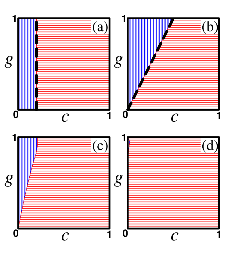
In Fig. 1, we draw C-rich and D-rich regions for BD by blue-vertical and red-horizontal lines respectively for four different values of selection intensities. C-rich regions in (a) and (b) are consistent with the analysis in the $wN$ limit [inequality (151)] and in the $Nw$ limit [inequality (153)] respectively. The dark-dashed lines, given by $c=1/5$ and $g=2c$ , are the boundaries between C-rich and D-rich regions predicted in the $wN$ and $Nw$ limits respectively. For $w=10$ shown in (d), defectors are more abundant for almost entire region. This is consistent with the $w\rightarrow\infty$ analysis which always predict $x_{\!{}_{D}}>x_{\!{}_{C}}$ for $n=1$ . For the intermediate value of $w=1$ shown in (c), we do not know the analytic boundary but we observe that the numerical boundary lies between the boundary for $w=10^{-2}$ of (b) and that for $w=10$ of (d) as expected.

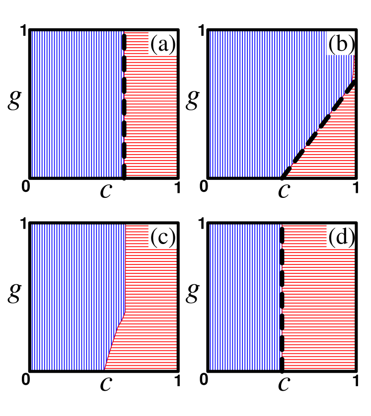
For DB, we show C-rich and D-rich regions for $N=10^{4}$ in Fig. 2. As in Fig. 1, they are represented by blue-vertical and red-horizontal lines respectively for four different values of selection intensities. C-rich regions in (a) and (b) coincide with the predictions for the $wN$ and $Nw$ limits respectively. The dark-dashed lines, given by $c=7/11$ and $g=\frac{4}{3}\left({c-\frac{1}{2}}\right)$ , are the boundaries between C-rich and D-rich regions predicted in the $wN$ and $Nw$ limits respectively. For $w=10$ shown in (d), cooperators are more abundant if $c<1/2$ as predicted in the $w\rightarrow\infty$ limit. As in the case of BD, we do not know the analytic boundary for the intermediate value of $w=1$ shown in (c). Yet, at least, we confirm that the numerical boundary lies between the boundary in the $Nw$ limit and that in the $w\rightarrow\infty$ limit.

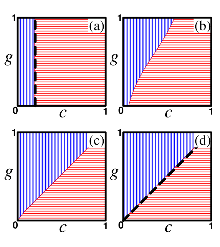
In Fig. 3, we show C-rich and D-rich regions for MP by blue-vertical and red-horizontal lines respectively. For MP, we do not have an analytic expression for the fixation probability in a closed form. Hence we need to calculate fixation probabilities directly from Eq. (52). Due to numerical cost for calculating abundance, which increases rapidly with $N$ , we investigate relatively small population of $N=100$ . However, they seem to be big enough to confirm the analytic prediction of the boundaries between C-rich and D-rich regions in the $wN$ limit and in the large $w$ limit. The dark-dashed lines in (a) and (d), given by $c=1/5$ and $g=c$ , are the predicted boundaries in the $wN$ and large $w$ limits respectively.

7.2 Combined effects of optionality and spatial structure

Now, let us compare the effects of the option to be loners on the structured population (BD and DB) to those on the well-mixed population (MP). It is immediately clear that the effects of spatial structure depend on the update rule. Comparing Figures 1 and 3, we see that BD updating does not support cooperation, in accordance with findings from other models (Ohtsuki & Nowak,, 2006; Ohtsuki et al.,, 2006; Hauert et al.,, 2014) In panels 1(a) and 3(a), where $Nw=0.1$ , the C-rich regions for BD and MP appear to coincide. This accords with our results that, in the $wN$ limit, the condition for $x_{C}>x_{D}$ is $c<b/5$ for both MP and BD (see Section 6). In the other panels of Figures 1 and 3, we see that the C-rich regions for BD are smaller than those for MP, suggesting that BD updating actually impedes cooperation relative to its success in a well-mixed population.

DB updating is generally favorable to cooperation, as can be seen by comparing Figures 2 and 3. In the $wN$ limit, for example, the condition for $x_{C}>x_{D}$ is $c<7b/11$ under DB updating (see Section 6), which is less stringent than the corresponding condition for MP, $c<b/5$ . These conditions correspond approximately to the C-rich regions shown in Figrues 2(a) and 3(a). However, we find that as $w$ increases, the C-rich regions for DB do not necessarily contain those for MP. In other words, for large selection intensity, there are parameter combinations under which cooperation is favored in a well-mixed population but disfavored on the cycle with DB updating. This effect is most visible in Figures 2(d) and 3(d), but it can also be seen in 2(c) and 3(c). In the $w\to\infty$ limit, we found (Section 6) that cooperation is favored for MP if $c<g$ , while it is favored for DB for $c<b/2$ . Either one of these conditions can be satisfied while the other fails, as can be seen (approximately) in Figures 2(d) and 3(d).

Optionality of the game and spatial structure (with DB updating) are two mechanisms that support cooperation. Do these mechanisms combine in a synergistic way? We find little evidence that they do. Let us consider first the $wN$ limit. With spatial structure alone (DB updating with $n=0$ loner strategies), cooperation succeeds if $c<b/2$ . With optionality alone (MP with $n=1$ ), cooperation succeeds if $c<b/5$ . With both optionality and spatial structure (DB with $n=1$ ), the condition is $c<7b/11$ , and we observe that the $7b/11$ threshold is less than the sum $b/2+b/5=7b/10$ of the thesholds corresponding to the the two mechanisms acting alone. The lack of synergy is even more apparent as the selection intensity $w$ increases, since, as noted above, there are parameter combinations for which cooperation is favored for MP but disfavored for DB.

7.3 Effects of selection intensity

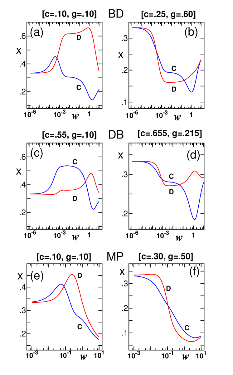
Let us now take a closer look at the effects of selection intensity. As shown in Fig. 1-3, the boundary between $C$ -rich region and $D$ -rich region changes as the selection intensity, $w$ varies. In other words, selection intensity may switch the rank of strategy abundance for some regions of parameter space as recently reported (Wu et al.,, 2013). In Fig. 4, we show selection intensity dependence of abundance for a couple of different pairs of $c$ and $g$ . Abundance is numerically calculated using Eq. (71) with $N=10^{4}$ for BD and DB. For MP, we consider $N=100$ due to numerical cost. In the left panels, we choose parameters $c$ and $g$ such that cooperators are more abundant than defectors ( $x_{\!{}_{C}}>x_{\!{}_{D}}$ ) in the $wN$ limit but change abundance order ( $x_{\!{}_{D}}>x_{\!{}_{C}}$ ) in the $Nw$ limit (for BD and DB) or large $w$ limit (for MP). For (a) BD, (c) DB, and (e) MP, we choose $(c,g)=(0.1,0.1)$ , $(0.55,0.1)$ , and $(0.1,0.1)$ respectively and find “crossing intensity”, $w_{c}$ . Population remains as $C$ -rich phase for $w<w_{c}$ where $w_{c}$ is around 0.0005, 0.4, and 0.08 for (a), (c), and (e) respectively. In the right panels, we consider the opposite cases and choose parameters such that defectors are more abundant in the $wN$ limit but becomes less abundant in the $Nw$ limit (for BD and DB) or large $w$ limit (for MP). For (b) BD, (d) DB, and (f) MP, we choose $(c,g)=(0.25,0.6)$ , $(0.655,0.215)$ , and $(0.3,0.5)$ respectively. For BD and DB, cooperators seem to be more abundant only in the $Nw$ limit. They are less abundant than defectors for large $w$ limit as well as in the $wN$ limit. In other words, there are two crossing intensities, $w_{c_{1}}$ and $w_{c_{2}}$ , such that $x_{\!{}_{C}}$ is larger than $x_{\!{}_{D}}$ only for $w_{c_{1}}<w<w_{c_{2}}$ . They are given by $w_{c_{1}}=0.0003$ and $w_{c_{2}}=0.25$ for (b) and $w_{c_{1}}=0.001$ and $w_{c_{2}}=0.04$ for (d). For MP shown in (f), there seems to be only one crossing point around at $w=0.1$ .

7.4 Simulation with finite mutation rate

Abundance of Eq. (71) is calculated in the low mutation limit using the fixation probabilities. After the invasion of a mutant to the mono-strategy population, the possibility of further mutation during the fixation is ignored. Strictly speaking, this is valid only when the mutation rate $u$ goes to zero. Here, we measure the abundance of three strategies, $x_{\!{}_{C}}$ , $x_{\!{}_{D}}$ , and $x_{\!{}_{L}}$ by Monte Carlo simulations with a small but finite mutation rate and compare them with abundance of Eq. (71).

We start from a random arrangement of three strategies $C$ , $D$ , and $L$ on a cycle (BD and DB) or a complete graph (MP) with $N$ sites. Population evolves with BD, DB, or MP updating. The mutation probability of the offspring is $u$ ; it bears its parent strategy with probability $1-u$ and takes one of the other two strategies with probability $u$ . In the mutation process, both strategies have equal chances, i.e., probability of $u/2$ for each.

To get statistical properties, we perform $M=6\times 10^{4}$ independent simulations and calculate the average frequencies of strategies. We monitor the time evolution of the average frequencies and see if the population evolves to a steady state in which average frequency remains constant. In the ensemble of steady states, we believe that the probability distribution of frequencies are stationary. For a single simulation, frequencies in the population may oscillate through mutation-fixation cycles for small mutation rates. However, the ensemble average of $M$ independent simulations effectively provides mean frequencies equivalent to time average over many fixations. We call this mean frequency as abundance.

Time to reach a steady state from the random initial configuration increases rapidly with population size $N$ . Hence, we simulate relatively small population of $N=50$ . We use mutation rate $u=0.0002$ such that $Nu=0.01$ in all simulations.

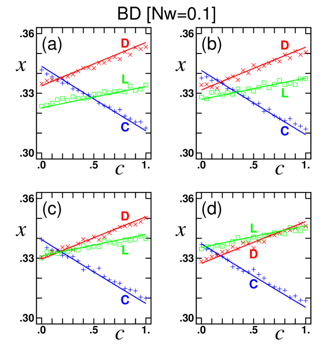
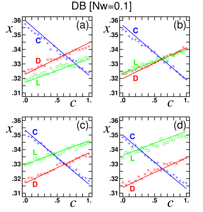
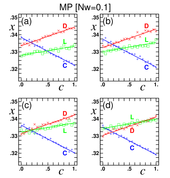
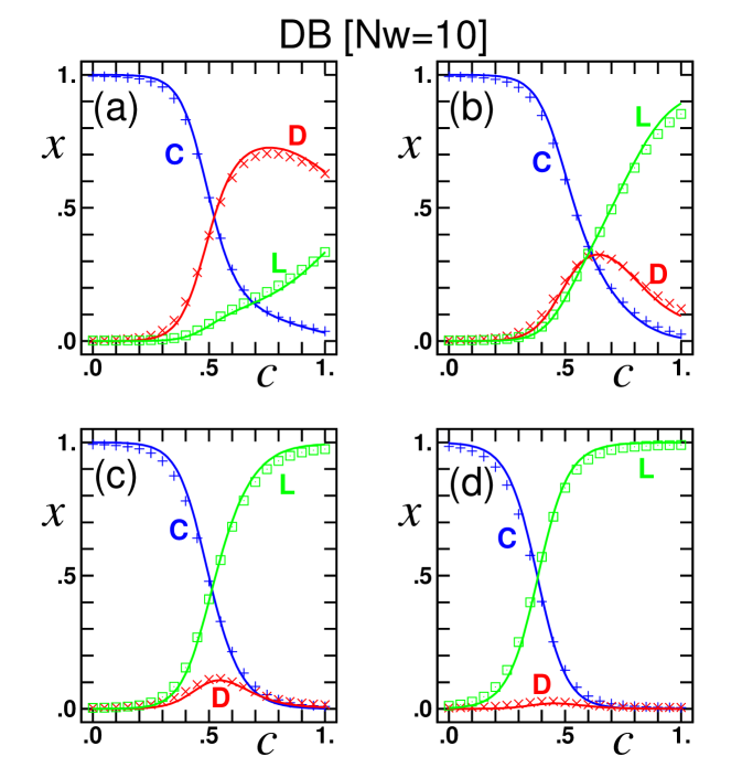
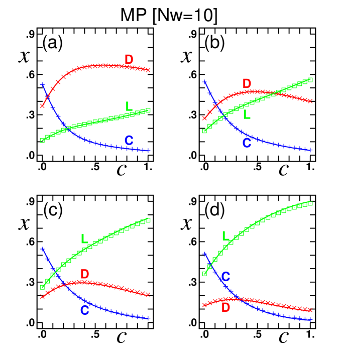
We first measure abundance of cooperators, $x_{\!{}_{C}}$ , defectors, $x_{\!{}_{D}}$ , and loners, $x_{\!{}_{L}}$ in the small $Nw$ regime with $Nw=0.1$ . Abundance versus cost, $x$ - $c$ plots are shown in Fig. 5, 6, and 7 for BD, DB, and MP respectively. For each updating process, we simulate population dynamics with 21 different values of $c$ , $c=0.$ , 0.05, $\ldots$ , 1, for each of four different values of $g$ , (a) 0, (b) 0.2, (c) 0.4, and (d) 0.6. Blue plus, red cross, and green square symbols represent the $x_{\!{}_{C}}$ , $x_{\!{}_{D}}$ , and $x_{\!{}_{L}}$ respectively. They are compared with abundance of Eq. (71), calculated using fixation probabilities, which are represented by blue, red, and green solid lines. We first note that the abundance of all strategies are around 1/3 as expected in the $wN$ limit. Measured data from simulations are consistent with abundance of Eq. (71) except a tiny but systematic deviation. When abundance is larger than 1/3, measured data tend to stay below the lines while they seem to stay above the lines when it is smaller than 1/3. These deviations seem to come from the fact that we use finite mutation rate ( $u=0.0002$ ) instead of infinitesimal rate. Random mutations make abundance move to the average value (1/3) regardless of its strategy. Except this small discrepancy, simulation data seem to follow all features of calculated abundance of Eq. (71). For example, $x_{\!{}_{D}}$ and $x_{\!{}_{L}}$ increase linearly and $x_{\!{}_{C}}$ decreases linearly with increasing $c$ . Especially, we note that crossing points of $x_{\!{}_{C}}$ and $x_{\!{}_{D}}$ are independent of $g$ as predicted. $x_{\!{}_{C}}$ and $x_{\!{}_{D}}$ meet near $c=1/5$ for BD and MP, and near $c=7/11\simeq 0.64$ for DB.

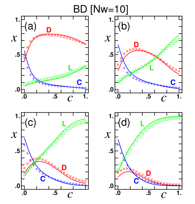
Simulation data for the large $Nw$ also follow the predicted abundance of Eq. (71) quite well. Figures 8, 9 and and 10 show $x$ - $c$ plots for BD, DB, and MP respectively for $w=0.2$ ( $Nw=10$ ). As before, $x_{\!{}_{C}}$ , $x_{\!{}_{D}}$ , and $x_{\!{}_{L}}$ versus $c$ graphs are represented by blue plus, red cross, and green square symbols respectively for four different values of $g$ , (a) 0, (b) 0.2, (c) 0.4, and (d) 0.6. They are compared with calculated abundance of Eq. (71), shown by blue, red, and green solid lines. As before, we observe small but systematic discrepancies between simulation data and predicted abundance of Eq. (71). Measure abundance deference between (different) strategies are smaller than the predictions. This can be understood from the fact that mutations reduce the abundance difference between strategies. Aside from this systematic deviation, simulation data follow the features of predicted abundance very well.

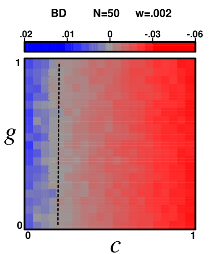
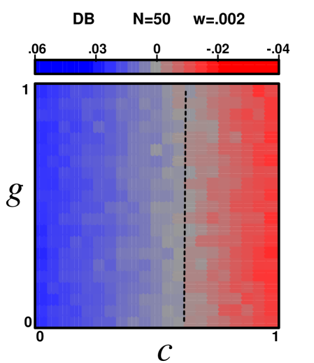
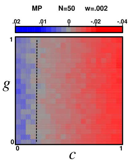
We now investigate C-rich and D-rich regions in the parameter space of $c$ and $g$ and compare them with those in the low mutation limit. We first measure $x_{\!{}_{C}}$ and $x_{\!{}_{D}}$ for $21\times 21$ different $c$ - $g$ pairs in $r\in[0\ 1]$ and $g\in[0\ 1]$ with intervals of 0.05. Then, we plot a normalized abundance difference between cooperators and defectors, $r=(x_{\!{}_{C}}-x_{\!{}_{D}})/(x_{\!{}_{C}}+x_{\!{}_{D}})$ in color in $21\times 21$ mesh in the $c$ - $g$ parameter space (Figs. 11 and 12) to illustrate C-rich and D-rich regions. As before, we use population of $N=50$ with mutation rate $u=0.0002$ . The blue-vertical and the red-horizontal paintings represent C-rich and D-rich regions respectively.

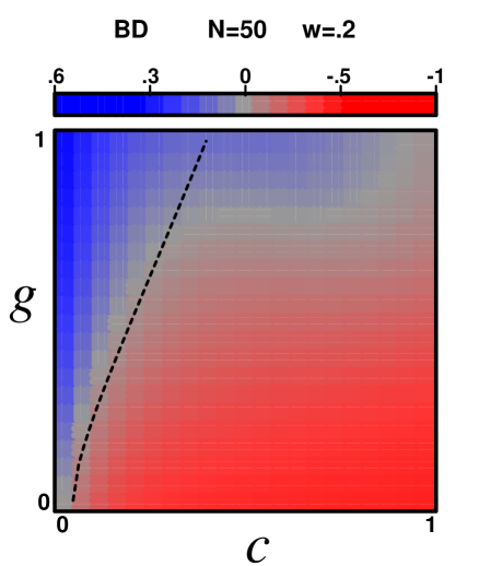
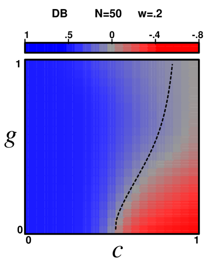
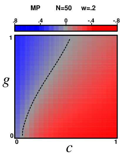
Figure 11 shows the normalized abundance difference, $r$ in the small $Nw$ regime for the three processes with $w=0.002$ ( $Nw=0.1$ ). As predicted by the panels (a) in Fig. 1-3, blue-rich region changes to red-rich region as $c$ increases, more or less, uniformly regardless of $g$ values. The phase boundaries calculated in the low mutation limit are shown in black-dashed lines. Those lines locate near $c=1/5$ for BD and MP and near $c=7/11$ for DB updating and they are consistent to the boundaries between two colors.

Boundaries (of C-rich and D-rich regions) obtained from the simulations for the large $Nw$ regime are also consistent with those calculated in the low mutation limit. Figure 12 shows the normalized abundance difference, $r$ in color for the three processes with $w=0.2$ ( $Nw=10$ ) in the $c$ - $g$ parameter space. As in Fig. 11, the blue-vertical and the red-horizontal paintings represent C-rich and D-rich regions respectively. The phase boundaries calculated in the low mutation limit are shown in black-dashed lines. They are consistent with color boundaries quite well expect for large $g$ for BD updating. We observe that cooperators favored over defectors for wider range of $c$ for large $g$ for BD updating. However, the absolute abundance of cooperators is small (although it is still larger than $x_{\!{}_{D}}$ ) when $g$ is large, since loners prevail the population.

8 Conclusion

We have analyzed strategy selection in optional games on cycles and on complete graphs and found a non-trivial interaction between volunteering and spatial selection.

For $2\times 2$ games on cycles using exponential fitness, we have presented a closed form expression for the fixation probability for any intensity of selection and any population size. Using this fixation probability, we have found the conditions for strategy selection analytically in the limits of weak intensity of selection and large population size. We have presented results for two orders of limits: (i) $w\to 0$ followed by $N\to\infty$ (which we call the $wN$ -limit) and (ii) $N\to\infty$ followed by $w\to 0$ (which we call the $Nw$ -limit). In the first case we have $wN\ll 1$ ; in the second we have $Nw\gg 1$ . We have also obtained numerical results for finite $w$ in the low mutation limit.

According to our observations, increasing the number of loner strategies relaxes the social dilemma and promotes evolution of cooperation. Increasing the number of loner strategies is equivalent to increasing mutational bias toward loner strategies. More loner strategies (or equivalently, more bias in mutation toward loners) favors cooperation by enabling loners to invade defector clusters and facilitate the return of cooperators. In the limit of an infinite number of loner strategies the social dilemma is completely resolved for any selection intensity. For high intensity of selection ( $w\gg 1$ ), the social dilemma can be fully resolved if there is mutational bias toward loner strategies (or there are more than one loner strategies).

While optionality of the game and spatial population structure both support cooperation, we have not found evidence of synergy between these mechanisms. This lack of synergy appears due to the fact that these mechanisms act in different ways. Spatial structure supports cooperation by allowing cooperators to isolate themselves, while optionality supports cooperation by allowing loners to infiltrate defectors. Neither mechanism appears to improve the efficacy of the other. In fact, for strong selection (the $w\to\infty$ limit) these mechanisms appear to counteract one another, in that there are parameter combinations for which coopeation is favored in the well-mixed population but disfavored for DB updating on the cycle.

We speculate that the role of loner strategies in relaxing social dilemmas, which we observe in our study, is qualitatively valid for games on general graphs. Since the population structures in our study, cycles and complete graphs, are at the two extreme ends of the spectrum of spatial structures, we expect loner strategies in optional games on other graphs also to relax social dilemma. The relaxation effect of volunteering increases as more loner strategies are available.

9 Acknowledgments

Support from the program for Foundational Questions in Evolutionary Biology (FQEB), the National Philanthropic Trust, the John Templeton Foundation and the National Research Foundation of Korea grant (NRF-2010-0022474) is gratefully acknowledged.

References

Allen et al., (2013) Allen, B., Gore, J., Nowak, M. A. & Bergstrom, C. T. 2013. Spatial dilemmas of diffusible public goods. eLife, 2, e01169.
Allen & Nowak, (2014) Allen, B. & Nowak, M. 2014. Games on graphs. EMS Surv. Math. Sci. 1 (1), 113–151.
Batali & Kitcher, (1995) Batali, J. & Kitcher, P. 1995. Evolution of altriusm in optional and compulsory games. J Theor Biol, 175, 161–171.
Boyd & Richerson, (1992) Boyd, R. & Richerson, P. J. 1992. Punishment allows the evolution of cooperation (or anything else) in sizable groups. Ethology and Sociobiology, 13 (3), 171–195.
Challet & Zhang, (1997) Challet, D. & Zhang, Y.-C. 1997. Emergence of Cooperation and Organization in an Evolutionary Game. Physica A-Statistical Mechanics and Its Applications, 246, 407–418.
Cressman, (2003) Cressman, R. 2003. Evolutionary Dynamics and Extensive Form Games. MIT Press, Cambridge.
De Silva et al., (2009) De Silva, H., Hauert, C., Traulsen, A. & Sigmund, K. 2009. Freedom, enforcement, and the social dilemma of strong altruism. J Evol Econ, 20 (2), 203–217.
Foster & Young, (1990) Foster, D. & Young, P. 1990. Stochastic evolutionary game dynamics. Theor Popul Biol, 38 (2), 219–232.
Friedman, (1998) Friedman, D. 1998. On economic applications of evolutionary game theory. J Evol Econ, 8 (1), 15–43.
(10) Fu, F., Chen, X., Liu, L. & Wang, L. 2007a. Social dilemmas in an online social network: The structure and evolution of cooperation. Phys Lett A, 371 (1-2), 58–64.
(11) Fu, F., Chen, X., Liu, L. & Wang, L. 2007b. Promotion of cooperation induced by the interplay between structure and game dynamics. Physica A-Statistical Mechanics and Its Applications, 383 (2), 651–659.
Garcia & Traulsen, (2012) Garcia, J. & Traulsen, A. 2012. The structure of mutations and the evolution of cooperation. Plos One, 7 (4), e35287.
Gokhale & Traulsen, (2011) Gokhale, C. S. & Traulsen, A. 2011. Strategy abundance in evolutionary many-player games with multiple strategies. J Theor Biol, 283 (1), 180–191.
Hauert, (2002) Hauert, C. 2002. Volunteering as Red Queen Mechanism for Cooperation in Public Goods Games. Science, 296 (5570), 1129–1132.
Hauert et al., (2002) Hauert, C., De Monte, S., Hofbauer, J. & Sigmund, K. 2002. Replicator dynamics for optional public good games. J Theor Biol, 218 (2), 187–194.
Hauert et al., (2014) Hauert, C., Doebeli, M. & barre, F. D. e. 2014. Social evolution in structured populations. Nat Commun, 5, 3409.
Hauert et al., (2006) Hauert, C., Michor, F., Nowak, M. A. & Doebeli, M. 2006. Synergy and discounting of cooperation in social dilemmas. J Theor Biol, 239 (2), 195–202.
Hauert et al., (2007) Hauert, C., Traulsen, A., Brandt, H., Nowak, M. A. & Sigmund, K. 2007. Via Freedom to Coercion: The Emergence of Costly Punishment. Science, 316 (5833), 1905–1907.
Hilbe & Sigmund, (2010) Hilbe, C. & Sigmund, K. 2010. Incentives and opportunism: from the carrot to the stick. P R Soc B, 277 (1693), 2427–2433.
Hofbauer & Sigmund, (1998) Hofbauer, J. & Sigmund, K. 1998. Evolutionary Games and Population Dynamics. Cambridge University Press.
Hofbauer & Sigmund, (1988) Hofbauer, J. & Sigmund, K. S. 1988. The theory of evolution and dynamical systems. Cambridge University Press.
Imhof & Nowak, (2006) Imhof, L. A. & Nowak, M. A. 2006. Evolutionary game dynamics in a Wright-Fisher process. J. Math. Biol. 52 (5), 667–681.
Kitcher, (1993) Kitcher, P. 1993. The evolution of human altruism. The Journal of Philosophy, 90 (10), 497–516.
Lieberman et al., (2005) Lieberman, E., Hauert, C. & Nowak, M. A. 2005. Evolutionary dynamics on graphs. Nature, 433 (7023), 312–316.
Maciejewski, (2014) Maciejewski, W. 2014. Reproductive value in graph-structured populations. J Theor Biol, 340, 285–293.
Michor & Nowak, (2002) Michor, F. & Nowak, M. A. 2002. Evolution: The good, the bad and the lonely. Nature, 419 (6908), 677–679.
Nakamaru & Iwasa, (2005) Nakamaru, M. & Iwasa, Y. 2005. The evolution of altruism by costly punishment in lattice-structured populations: score-dependent viability versus score-dependent fertility. Evolutionary ecology research, 7, 853–870.
Nakamaru et al., (1997) Nakamaru, M., Matsuda, H. & Iwasa, Y. 1997. The Evolution of Cooperation in a Lattice-Structured Population. J Theor Biol, 184 (1), 65–81.
Nowak, (2004) Nowak, M. A. 2004. Evolutionary Dynamics of Biological Games. Science, 303 (5659), 793–799.
(30) Nowak, M. A. 2006a. Five Rules for the Evolution of Cooperation. Science, 314 (5805), 1560–1563.
(31) Nowak, M. A. 2006b. Evolutionary Dynamics: Exploring the Equations of Life. Harvard University Press, Cambridge.
Nowak, (2012) Nowak, M. A. 2012. Evolving cooperation. J Theor Biol, 299, 1–8.
Nowak et al., (1994) Nowak, M. A., Bonhoeffer, S. & May, R. M. 1994. Spatial games and the maintenance of cooperation. Proceedings of the National Academy of Sciences, 91, 4877–4811.
Nowak & May, (1992) Nowak, M. A. & May, R. M. 1992. Evolutionary games and spatial chaos. Nature, 359, 826–829.
Nowak et al., (2004) Nowak, M. A., Sasaki, A., Taylor, C. & Fudenberg, D. 2004. Emergence of cooperation and evolutionary stability in finite populations. Nature, 428 (6983), 646–650.
Nowak et al., (2010) Nowak, M. A., Tarnita, C. E. & Antal, T. 2010. Evolutionary dynamics in structured populations. Philosophical Transactions of the Royal Society B: Biological Sciences, 365 (1537), 19–30.
Ohtsuki et al., (2006) Ohtsuki, H., Hauert, C., Lieberman, E. & Nowak, M. A. 2006. A simple rule for the evolution of cooperation on graphs and social networks. Nature, 441 (25), 502–505.
Ohtsuki & Nowak, (2006) Ohtsuki, H. & Nowak, M. A. 2006. Evolutionary games on cycles. P R Soc B, 273 (1598), 2249–2256.
Perc, (2011) Perc, M. 2011. Does strong heterogeneity promote cooperation by group interactions? New J. Phys. 13 (12), 123027.
Perc & Szolnoki, (2010) Perc, M. & Szolnoki, A. 2010. Coevolutionary games—A mini review. Biosystems, 99 (2), 109–125.
Rand & Nowak, (2011) Rand, D. G. & Nowak, M. A. 2011. The evolution of antisocial punishment in optional public goods games. Nat Commun, 2, 434.
Rand & Nowak, (2013) Rand, D. G. & Nowak, M. A. 2013. Human cooperation. Trends in cognitive sciences, 17 (8), 413–425.
Santos & Pacheco, (2005) Santos, F. & Pacheco, J. 2005. Scale-Free Networks Provide a Unifying Framework for the Emergence of Cooperation. Phys. Rev. Lett. 95 (9), 098104.
Santos et al., (2008) Santos, F. C., Santos, M. D. & Pacheco, J. M. 2008. Social diversity promotes the emergence of cooperation in public goods games. Nature, 454 (7201), 213–216.
Sigmund, (2007) Sigmund, K. 2007. Punish or perish? Retaliation and collaboration among humans. Trends in Ecology & Evolution, 22 (11), 593–600.
Szabó & Fáth, (2007) Szabó, G. & Fáth, G. 2007. Evolutionary games on graphs. Physics Reports, 446 (4-6), 97–216.
(47) Szabó, G. & Hauert, C. 2002a. Evolutionary prisoner’s dilemma games with voluntary participation. Phys. Rev. E, 66 (6), 062903.
(48) Szabó, G. & Hauert, C. 2002b. Phase transitions and volunteering in spatial public goods games. Phys. Rev. Lett. 89 (11), 118101.
(49) Tarnita, C. E., Antal, T., Ohtsuki, H. & Nowak, M. A. 2009a. Evolutionary dynamics in set structured populations. Proceedings of the National Academy of Sciences, 106 (21), 8601–8604.
(50) Tarnita, C. E., Ohtsuki, H., Antal, T., Fu, F. & Nowak, M. A. 2009b. Strategy selection in structured populations. J Theor Biol, 259 (3), 570–581.
Tarnita et al., (2011) Tarnita, C. E., Wage, N. & Nowak, M. A. 2011. Multiple strategies in structured populations. Proceedings of the National Academy of Sciences, 108 (6), 2334–2337.
Taylor et al., (2004) Taylor, C., Fudenberg, D., Sasaki, A. & Nowak, M. A. 2004. Evolutionary game dynamics in finite populations. Bull. Math. Biol. 66 (6), 1621–1644.
Traulsen et al., (2009) Traulsen, A., Hauert, C., De Silva, H., Nowak, M. A. & Sigmund, K. 2009. Exploration dynamics in evolutionary games. Proceedings of the National Academy of Sciences, 106 (3), 709–712.
Traulsen et al., (2006) Traulsen, A., Pacheco, J. M. & Imhof, L. A. 2006. Stochasticity and evolutionary stability. Phys. Rev. E, 74, 021905.
Traulsen et al., (2008) Traulsen, A., Shoresh, N. & Nowak, M. A. 2008. Analytical Results for Individual and Group Selection of Any Intensity. Bull. Math. Biol. 70 (5), 1410–1424.
van Veelen & Nowak, (2012) van Veelen, M. & Nowak, M. A. 2012. Multi-player games on the cycle. J Theor Biol, 292, 116–128.
Vincent & Brown, (2005) Vincent, T. L. & Brown, J. S. 2005. Evolutionary Game Theory, Natural Selection, and Darwinian Dynamics. Cambridge University Press.
Weibull, (1997) Weibull, J. W. 1997. Evolutionary Game Theory. MIT Press.
Wu et al., (2013) Wu, B., Garcia, J., Hauert, C. & Traulsen, A. 2013. Extrapolating weak selection in evolutionary games. PLoS Comp Biol, 9 (12), e1003381.

Optional games on cycles and complete graphs

Abstract

1 Introduction

2 Model and main results

2.1 w​NwN limit

2.2 Nw limit

2.3 Numerical analysis

3 Derivation of general expressions for fixation probability and abundance

3.1 Fixation probability

3.2 Abundance in the low mutation limit

3.3 Optional prisoner’s dilemma game

4 Analysis of the w​NwN limit

4.1 Fixation probability

4.2 Strategy selection

4.3 Optional prisoner’s dilemma game

5 Analysis of the N​wNw limit

5.1 Fixation probability

5.2 Strategy selection

5.3 Optional prisoner’s dilemma game

6 Optional game with simplified prisoner’s dilemma

7 Numerical analysis

7.1 Numerical comparison of abundance of cooperators and defectors

7.2 Combined effects of optionality and spatial structure

7.3 Effects of selection intensity

7.4 Simulation with finite mutation rate

8 Conclusion

9 Acknowledgments

References

2.1 $wN$ limit

4 Analysis of the $wN$ limit

5 Analysis of the $Nw$ limit