Optomechanics with a position-modulated Kerr-type nonlinear coupling

The system we consider can be described by an extension of standard optomechanical setups, such as the membrane-in-the-middle model Bhattacharya2008 ; Thompson2008 ; Biancofiore2011 , where the membrane is modeled as a harmonic oscillator with a single mechanical frequency $\Omega_{m}$ and nondimensional position and momentum operators $(\hat{q},\hat{p})$. The cavity field is modeled as a harmonic oscillator and described by the bosonic creation and annihilation operators, $\hat{a}^{\dagger}$ and $\hat{a}$, which create photons with the resonant frequency $\omega_{0}$. The membrane and the cavity interact via radiation pressure, which pushes the membrane and therefore changes the resonance frequency, making it position dependent $\omega(\hat{q})$. Since the harmonic oscillator is described by $\hbar\omega(\hat{q})\hat{a}^{\dagger}\hat{a}$, this gives rise to a position-dependent interaction which is linear in the optical-field operators. While it is possible to perform the analytic treatment with no assumptions of the form of $\omega(\hat{q})$ Biancofiore2011 , we will consider the case of

from the beginning as this clarifies the relation between the two types of interaction we will consider. Within the linearity assumption the optomechanical interaction is then described as $\hat{H}_{\text{L,int}}=-\hbar\hat{a}^{\dagger}\hat{a}g_{\text{L}}\hat{q}$.

The second type of interaction we consider is nonlinear in the optical field operators, which corresponds to a simultaneous two-photon process that can be facilitated by a $\chi^{(3)}$ material and is described by the term $H_{\text{Kerr}}=\eta\hbar\hat{a}^{\dagger}\hat{a}^{\dagger}\hat{a}\hat{a}$. In order to obtain a position-dependent interaction with a moving membrane the nonlinear coefficient has to become dependent on its position $\eta(\hat{q})$. If this can be engineered, then the nonlinear coefficient will be given similarly to the linear coefficient as

Throughout the paper we will generally use the dimensionless position-coordinate $\hat{q}$, but in order to derive the values of these coefficients for a specific physical system, it is easier to use the dimensional position coordinate $\hat{x}$, which is related to the nondimensional coordinate by some characteristic length scale $x_{0}$ as $\hat{q}=\hat{x}/x_{0}$. Correspondingly, one can relate coupling strengths for the nondimensional coordinates to those of the dimensional coordinates by $g_{\text{NL}}=x_{0}G_{\text{NL}},g_{\text{L}}=x_{0}G_{\text{L}}$. The characteristic length scale in optomechanics is generally the zero-point motion of the mechanical element $x_{\text{zp}}$ RevModPhys.86.1391 .

The optomechanical setup we are considering is an open system and interactions with the environment in the form of photon losses, mechanical dissipation, and noise have to be taken into account. We do this by utilizing the quantum Langevin formalism and consider photon loss associated with the end mirrors of the cavity $\kappa_{0}$ and photon loss associated with a moving element, such as a membrane $\kappa_{1}(\hat{q})$. While experimental evidence suggest that the dependence of $\kappa_{1}(\hat{q})$ on the position is usually small Karuza2012 , we take it into account to get the most general picture. The losses have associated noise operators $\hat{a}_{0}^{in}$ and $\hat{a}_{1}^{in}$, which have the correlation relation Biancofiore2011

In addition to the losses associated with the optical field, mechanical dissipation of the membrane $\gamma_{m}$ must be considered. For this the associated noise operator has the correlation relation

where $\nu$ is the Fourier space frequency and

is the mean phonon number at temperature $T_{0}$ and $\delta^{\prime}(t-t^{\prime})$ is the derivative of the Dirac-delta function. Adding these to the Heisenberg equations for the Hamiltonian (4) we arrive at the quantum Langevin equations (QLE)

The $\partial_{q}\kappa_{1}(\hat{q})$ term is an effective noise term arising from the absorption in the membrane, as long as it is not assumed constant Biancofiore2011 . Solving this full set of quantum-mechanical equations is not a trivial task and we therefore employ a semiclassical approximation where we assume the physical operators can be expressed as a classical average $\{q,p,\alpha\}$ plus some small quantum fluctuation $\{\delta\hat{q},\delta\hat{p},\delta\hat{a}\}$

This assumption only holds when the classical part is large, which is the situations experiments are commonly in. In the next section we will look at various aspects of the solutions for the system.

To determine the classical steady-state solutions we consider the quantum fluctuations to be small compared to the classical c-numbers, so that any terms containing them can be neglected. Setting all derivatives in the QLE to zero then leads to

where $\kappa(q_{s})=\kappa_{0}+\kappa_{1}(q_{s})$. Assuming that $\kappa_{1}(q_{s})=\kappa_{\text{L}}q_{s}$ these two coupled equations can be expressed as a single seventh-order polynomial for the mean photon number $n_{s}=|\alpha_{s}|^{2}$ of the form

Even though this seventh-order polynomial equation has in principle seven roots, all complex solutions can be discarded as the mean photon number has to be real. The steady-state position of the membrane can then be found by inserting the resulting solution for $n_{s}$ into expression (12). We note that doing a similar analysis for the linear system leads to a third-order polynomial only.

To determine the stability of the steady-state solutions and to calculate physical values that depend solely on the quantum fluctuations, such as the temperature of the membrane, we will in this section look at the effects of the fluctuation terms. For this we use the quadratures of the electric field $\hat{\delta X}=(\delta\hat{a}+\delta\hat{a}^{\dagger})/\sqrt{2}$ , $\hat{\delta Y}=(\delta\hat{a}-\delta\hat{a}^{\dagger})/\sqrt{2}i$, $\hat{X}^{in}_{j}=(\hat{a}_{j}^{in}+\hat{a}_{j}^{in\dagger})/\sqrt{2}$ and $\hat{Y}^{in}_{j}=(\hat{a}_{j}^{in}-\hat{a}_{j}^{in\dagger})/\sqrt{2}i$ and insert the steady-state solution plus the quantum-fluctuations into the QLEs. We are still considering the quantum fluctuations and the noise operators to be small and therefore only keep terms up to first order in these operators. This leads to the linearized quantum Langevin equations (LQLE) of the form

where we have defined the effective loss rate due to the position-dependent $\kappa_{1}(\hat{q})$ as $\Gamma=\sqrt{2}\partial_{q}\kappa_{1}(q_{s})\alpha_{s}$ and the overall effective coupling in the system as $G=\sqrt{2}\alpha_{s}(g_{\text{L}}+2g_{\text{NL}}|\alpha_{s}|^{2})$. Additionally we have defined the effective detuning $\Delta(q_{s})=\Delta-g_{\text{L}}q_{s}$. It is worth noting that the nonlinear coupling enters the effective coupling scaled with the mean photon number in the cavity and it can therefore be expected to have a much stronger effect than the linear coupling.

The LQLE can be rewritten as the matrix equation of the form

where

and

The drift matrix is given by

and can be seen to reduce to the linear drift matrix for $g_{\text{NL}}=0$ Biancofiore2011 . The four eigenvalues appear as complex conjugate pairs and give information about the quantum fluctuations in the system. Their real parts corresponds to the cooling (or heating rate) of the membrane and the cavity, which means that the system is only stable if both of these are negative and the system relaxes towards a steady state. The imaginary parts describe the dressed eigenfrequencies of the membrane and the optical field. The stationary state is characterized by the covariance matrix V, which is determined by the Lyapunov equation

and where D, known as the diffusion matrix, is related to the noise vector $c(t)$ by Biancofiore2011

It is explicitly given by Biancofiore2011

The mean occupation number for the phonons $n$ can be obtained from the mean energy of the mechanical resonator which is given by

where $V_{11}$ and $V_{22}$ are matrix elements from the covariance matrix.

The spectral function for the system is defined as Kumar2010

where $\nu$ is the Fourier space frequency. Taking the Fourier transformation of the LQLE one finds

where $C_{3}=C_{1}C_{2}-\delta G^{2}+(\kappa(q_{s})-i\nu)\Gamma,C_{1}=[\kappa(q_{s})-i\omega]^{2}+\delta^{\prime 2}$ and $C_{2}=\frac{\Omega_{m}^{2}+h\omega_{m}-\nu^{2}-i\nu\gamma_{m}}{\Omega_{m}}$ with $\delta^{\prime}(q_{s})^{2}=\Delta(q_{s})^{2}+12g_{\text{NL}}^{2}q_{s}^{2}-8\Delta(q_{s})g_{\text{NL}}q_{s}$ and $\delta(q_{s})=\Delta(q_{s})-2g_{\text{NL}}q_{s}$. Using the correlation relations for the noise operators in Fourier space then gives the spectrum

where the thermal and radiation pressure spectra are given by

and we have an extra noise spectrum associated with membrane absorption

Here $|\chi_{\text{eff}}|^{2}$ us the effective susceptibility and is given by

Again we note that the spectrum reduces to the linear one discussed in Ref. Biancofiore2011 if we assume that $g_{\text{NL}}=0$.

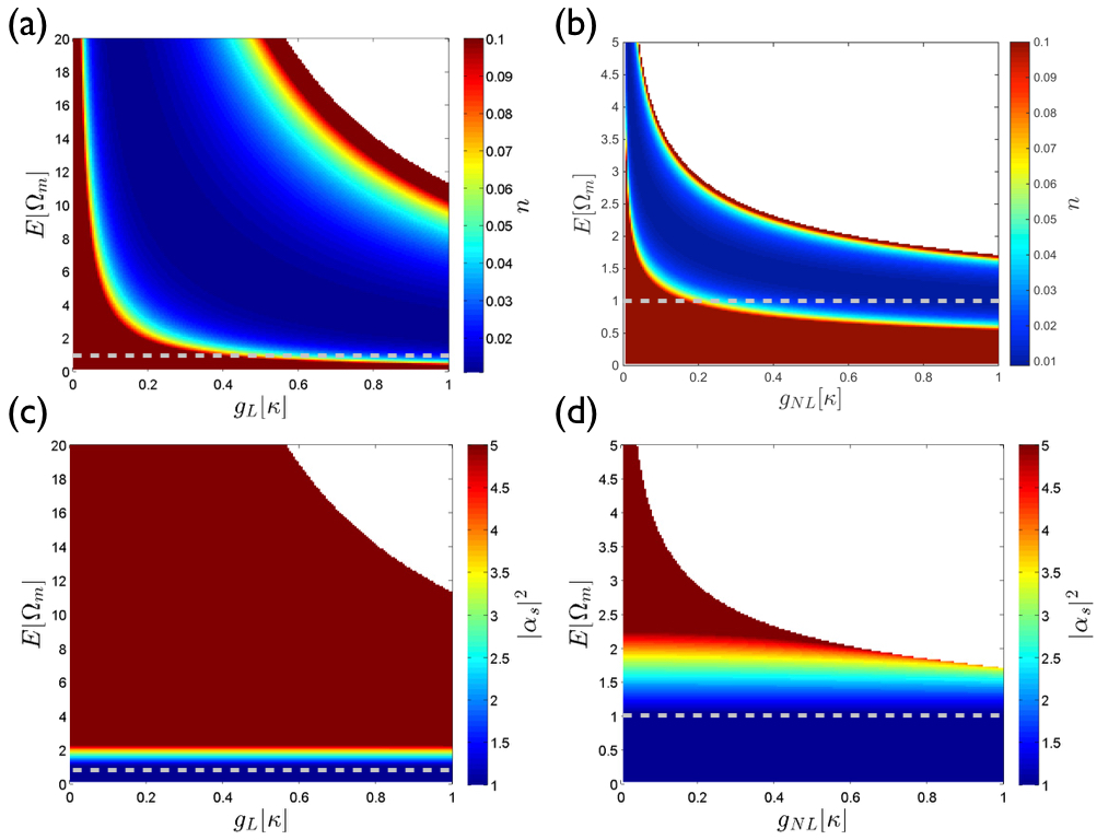
The phonon number as a function of the input energy of the laser and the linear and nonlinear couplings, respectively, for $\Delta=\Omega_{m}$ is shown in Figs. 1(a) 1(b). This corresponds to the resolved sideband regime where optimal cooling can be expected. One can see that for any value of $g_{\text{L}}$ or $g_{\text{NL}}$ there is a value of $E$ for which the same maximal cooling ($n\approx 0.01$) is obtained and this value reduces as the coupling strength is increased. In fact, the nonlinear coupling simply enhances this behavior that is already present in the linear case, reducing the value of $E$ required to achieve the same amount of cooling as in the linear case. Additionally one can see a rise in temperature as $E$ increases beyond the value for maximal cooling, until the solutions become unstable (white areas in the figures). The photon numbers for the same parameter ranges are plotted in Figs. 1(c) and 1(d). One can see that they generally increase with energy as one would expect; however, it is more relevant to confirm whether the photon number stays above 1 in the regime of relevance, i.e., the regime of maximal cooling, since our model is otherwise inapplicable. In fact, for very small values of $E$ it drops below 1 and to get maximal cooling for large values of $g_{\text{NL}}$, values of $E$ approaching this inapplicable regime must be chosen. For the most part, however, this limitation does not pose a problem. Situations where both $(g_{\text{L}}$ and $g_{\text{NL}})$ are finite behave similarly to the two limiting cases discussed here.

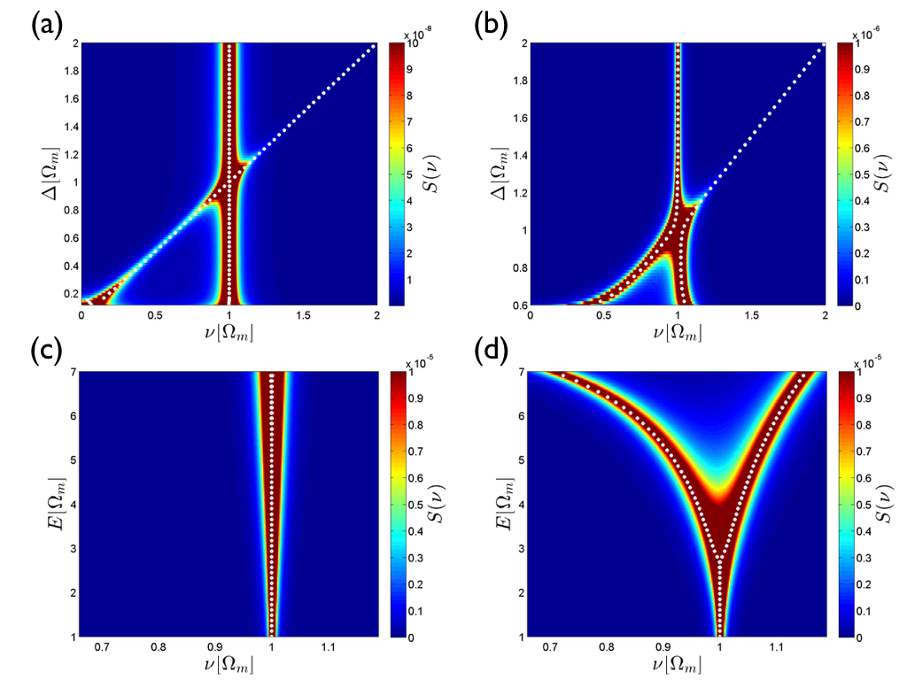
To investigate the existence of a strong-coupling regime at small laser intensities, we will look next at the spectrum $S(\nu)$ for $(g_{\text{L}},g_{\text{NL}})=(0.1\kappa,0)$ and $(g_{\text{L}},g_{\text{NL}})=(0.1\kappa,0.01\kappa)$. In both cases we have a fairly weak linear coupling and therefore do not expect the first case to be in the strong-coupling regime. The spectrum as a function of the detuning $\Delta$ at $E=4\Omega_{m}$ is plotted in Figs. 2(a) and 2(b), and one can see that without the nonlinear coupling the system is indeed in the weak-coupling regime (no splitting is visible). However, adding a comparatively small amount of nonlinear coupling, $g_{\text{NL}}=0.1g_{\text{L}}$, brings the system into the strong-coupling regime, signified by the avoided crossing of the dressed eigenfrequencies. This is quite remarkable as it allows for strong coupling at much smaller laser energies by adding just a small nonlinearity to the system. The spectrum as a function of the energy $E$ at $\Delta=\Omega_{m}$, is plotted in Figs. 2(c) and 2(d), where the normal-mode splitting for the nonlinear coupling $g_{\text{NL}}=0.1g_{\text{L}}$ is distinctly visible and clearly absent for the linear case at these energies. The figures also shows that our results are self-consistent as the imaginary part of the eigenvalues of the drift matrix $A$ (dotted white lines) correspond to the two peak positions in frequency space.

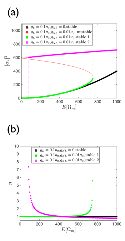
Another situation where the dramatic effect of a small nonlinearity becomes visible is shown in Fig. 3(a). Here the photon number is given as a function of $E$ for $(g_{\text{L}},g_{\text{NL}})=(0.1\kappa,0)$ and $(g_{\text{L}},g_{\text{NL}})=(0.1\kappa,0.01\kappa)$ at $\Delta=50\Omega_{m}$. The linear system can be seen to have only one solution in the displayed energy range, but adding the small nonlinearity leads to optical bistability as evidenced by the characteristic S-shaped curve. Starting at $E=0$ and slowly increasing the energy the system moves along the first stable solution with the smallest number of photons. When this solution becomes unstable there is a first order transition to the second stable solution which has the largest number of photons. If the energy is then decreased the system stays in this second steady state until it becomes unstable at which point a first-order transition to the first steady state takes place. This is the characteristic signature of optical hysteresis. In Fig. 3(b) the corresponding phonon numbers are plotted. The temperature (phonon number) of the solutions are fairly constant in the stable regimes but rise rapidly as a solution becomes unstable.

It is worth stressing again that this optical bistability appears at quite low energies, because the nonlinearity leads to strong effective coupling. To see bistability with linear coupling only, much larger energies would be needed.

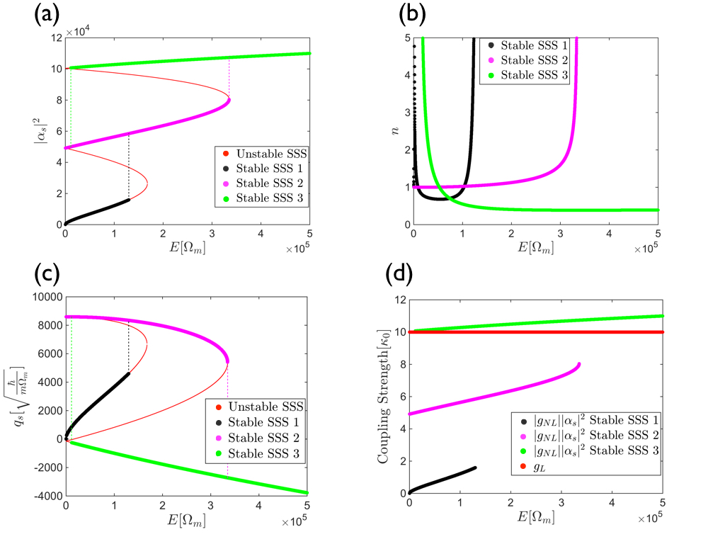
While we have shown above that choosing the linear and the nonlinear coupling strength to have the same sign leads to mostly an enhancement of the effects already present in the linear case, qualitatively new effects can appear when they have opposite signs. For this we consider in the following $(g_{\text{L}},g_{\text{NL}})=(10\kappa,-10^{-4}\kappa)$ and $\Delta=50\Omega_{m}$. The reason for the large difference between the linear and the nonlinear coupling strength is that if the couplings were chosen to be of comparable size, the nonlinear coupling will dominate the system as it enters the effective coupling scaled with the photon number, i.e., $G=\sqrt{2}\alpha_{s}(g_{\text{L}}+2g_{\text{NL}}|\alpha_{s}|^{2})$. Therefore, in order to engineer competition between the two forces, values for which the contribution of the nonlinear coupling $g_{\text{NL}}|\alpha_{s}|^{2}$ and the linear coupling $g_{\text{L}}$ are comparable must be chosen. In Fig. 4 we show the behavior of $|\alpha_{s}|^{2},n,q_{s},$ and $g_{\text{NL}}|\alpha_{s}^{2}$. Five steady-state solutions can be found, but only three of them are stable. To ease the discussion we will denote the three stable branches as 1, 2, and 3, where 1 corresponds to the stable solution with the smallest number of photons, 2 corresponds to the middle solution, while 3 corresponds to the solution with largest photon number [see Fig. 4(a)]. For increasing $E$, starting from $E=0$ the system will be in a state on the first branch, jump to the second branch at energies where the first branch is no longer stable, before finally moving to the third branch. Looking at the position of the membrane for these states, one can see from Fig. 4(c) that it moves in the positive direction along the first branch, then changes direction and moves in the negative direction along the second branch, and, finally, jumps to a negative value moving in the negative direction when the system enters the third branch. This means that as the system jumps from the second to the third branch, the position of the membrane should jump from being displaced in the positive direction to being displaced in the negative one. Since $q_{s}=(g_{\text{L}}+g_{\text{NL}}|\alpha_{s}|^{2})\frac{|\alpha_{s}|^{2}}{\Omega_{m}}$ one can understand this behavior by looking at the size of $g_{\text{L}}$ and $g_{\text{NL}}|\alpha_{s}|^{2}$, which is plotted in Fig. 4(d). Along the first branch $g_{\text{L}}$, which is positive, is dominant and so the membrane is pushed in the positive direction. Along the second branch $g_{\text{NL}}|\alpha_{s}|^{2}$, which depends on the photon number, becomes comparable with $g_{\text{L}}$ and though $q_{s}$ stays positive the effective coupling $G$ becomes negative. Increasing values of $E$ mean an effective decrease in the (positive) position $q_{s}$. On the third branch $g_{\text{NL}}|\alpha_{s}|^{2}$ is always much larger than $g_{\text{L}}$ and therefore the membrane has a negative effective coupling, while also being at a negative value in position space. This means that the system moves between attractive and repulsive regimes for the interaction between the membrane and the cavity field as it jumps between stable solutions. Finally, looking at the phonon number in Fig. 4(b), one can see that the temperature (phonon number) of the second branch is considerably higher than that of the other two, with the third branch having the lowest temperature.

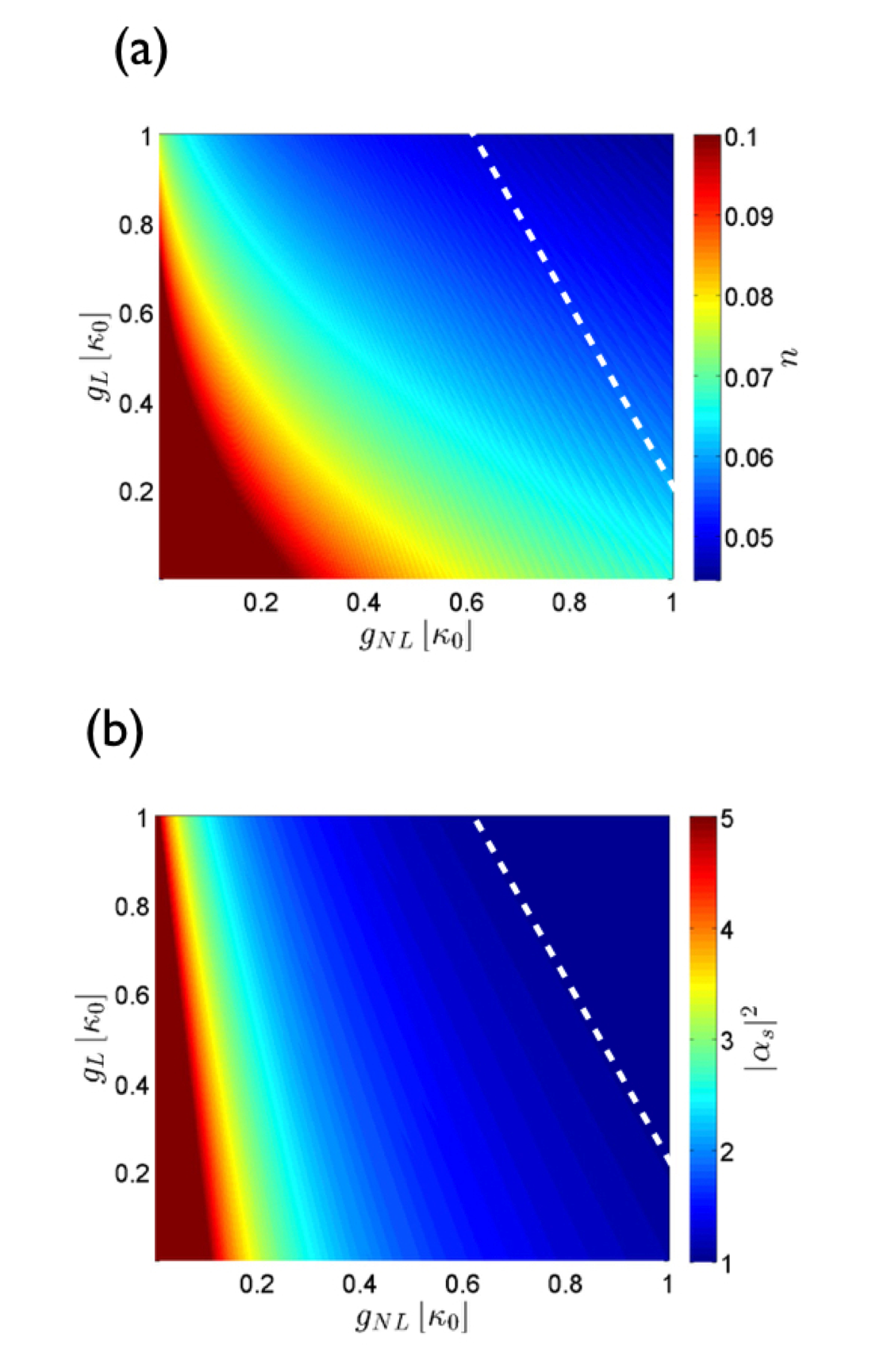
Finally we consider the case of letting the membrane absorption depend on the position, i.e., $\kappa_{1}(\hat{q})=\kappa_{\text{L}}\hat{q}$ with $\kappa_{\text{L}}=0.0130\kappa_{0}$ and $\kappa_{0}=77{\rm kHz}$, and study how this affects the cooling in the resolved sideband regime, where $\Delta=\Omega_{m}$. For this, the phonon number $n$ and the photon number $|\alpha_{s}|^{2}$ as a function of $g_{\text{NL}}$ and $g_{L}$ are shown in Fig. 5, where the energy at each point has been chosen so as to minimize $n$. One can see that the position dependent absorption coefficient leads to overall worse cooling [compare with $n\approx 0.01$ from Figs. 1 (a) and 1 (b)], which is to be expected. However, by increasing the coupling this trend can be counteracted, leading to more efficient cooling for a more strongly coupled system. As can be seen from Fig. 5 this favors the nonlinear coupling, which is always stronger than the linear coupling. Therefore in this case the nonlinear coupling can lead to more efficient cooling. Looking at the photon number however, one must be wary as the energy for which optimal cooling is obtained corresponds to photon numbers on the order of one for very strongly coupled systems. While this means that the basic assumption for our model breaks down, we find enhanced cooling for the majority of the investigated ranges without encountering this problem.

References

- (1) M. Aspelmeyer, T.J. Kippenberg and F. Marquardt, Rev. Mod. Phys. 86, 1391 (2008)
- (2) J.D. Teufel, T. Donner, D. Li, J.W. Harlow, M.S. Allman, K. Cicak, A.J. Sirois, J.D. Whittaker, K.W. Lehnert and R.W. Simmonds, Nature 475, 359 (2011)
- (3) J. Chan, T.P. Mayer Alegre, A.H. Safavi-Naeini, J.T. Hill, A. Krause, S. Groeblacher, M. Aspelmeyer and O. Painter, Nature 478, 89 (2011)
- (4) S. Weis, R. Rivi’ere, S. Del’eglise, E. Gavartin, O. Arcizet, A. Schliesser and T.J. Kippenberg, Science 330, 1520 (2010)
- (5) A.H. Safavi-Naeini, T.P.M. Alegre, J. Chan, M. Eichenfield, M. Winger, Q. Lin, J.T. Hill, D.E. Chang and O. Painter, Nature 472, 69 (2011)
- (6) D.W.C. Brooks, T. Botter, S. Schreppler, T.P. Purdy, N. Brahms and D.M. Stamper-Kurn, Nature 488, 476 (2012)
- (7) T.P. Purdy, P.L. Yu, R.W. Peterson, N.S. Kampel and C.A. Regal, Phys. Rev. X 3, 031012 (2013)
- (8) A.H. Safavi-Naeini, S. Groeblacher, J.T. Hill, J. Chan, M. Aspelmeyer and O. Painter, Nature 500, 185 (2013)
- (9) E.E. Wollman, C.U. Lei, A.J. Weinstein, J. Suh, A. Kronwald, F. Marquardt, A.A. Clerk and K.C. Schwab, Science 349, 952 (2015)
- (10) J.M. Pirkkalainen, E. Damskagg, M. Brandt, F. Massel and M.A. Sillanpaa, Phys. Rev. Lett. 115, 243601 (2015)
- (11) Y.D. Wang, and A.A. Clerk, Phys. Rev. Lett. 110, 253601 (2013)
- (12) T.A. Palomaki, J.D. Teufel, R.W. Simmondsand K.W. Lehnert, Science 342, 710 (2013)
- (13) V.C. Vivoli, T. Barnea, C. Galland and N. Sangouard, Phys. Rev. Lett. 116, 070405 (2016)
- (14) R. Riedinger, S. Hong, R.A. Norte, J.A. Slater, J. Shang, A.G. Krause, V. Anant, M. Aspelmeyer and S. Groblacher, Nature 530, 313 (2016)
- (15) M. Schmidt, M. Ludwig and F. Marquardt, New J. Phys. 14, 125005 (2012)
- (16) S. Rips and M.J. Hartmann, Phys. Rev. Lett. 110, 120503 (2013)
- (17) O. Houhou, H. Aissaoui and A. Ferraro, Phys. Rev. A 92, 063843 (2015)
- (18) S. Forstner, S. Prams, J. Knittel, E.D. van Ooijen, J.D. Swaim, G.I. Harris, A. Szorkovszky, W.P.Bowen and H. Rubinsztein-Dunlop, Phys. Rev. Lett. 108, 120801 (2012)
- (19) T. Bagci, A. Simonsen, S. Schmid, L.G. Villanueva, E. Zeuthen, J. Appel, J.M. Taylor, A. Sorensen, K. Usami, A. Schliesser and E.S. Polzik, Nature 507, 81 (2014)
- (20) M. Wu, A.C. Hryciw, C. Healey, D.P. Lake, H. Jayakumar, M.R. Freeman, J.P. Davis and P.E. Barclay, Phys. Rev. X 4, 021052 (2014)
- (21) S. Aldana, C. Bruder and A. Nunnenkamp, Phys. Rev. A 88, 043826 (2013)
- (22) M.R. Vanner, Phys. Rev. X 1, 021011 (2011)
- (23) T.K. Paraiso, M. Kalaee, L. Zang, H. Pfeifer, F. Marquardt and O. Painter, Phys. Rev. X 5, 041024 (2015)
- (24) G.A. Brawley, M.R. Vanner, P.E. Larsen, S. Schmid, A. Boisen and W.P. Bowen, Nature Comms. 7, 10988 (2016)
- (25) W. Xiong, D.-Y. Jin, Y. Qiu, C.-H. Lam and J. Q. You, Phys.Rev. A 93, 023844 (2016)
- (26) T. Kumar, A.B. Bhattacherjee and ManMohan Phys.Rev.A 81, 013835 (2010)
- (27) S. Shahidani, M.H. Naderi and M. Soltanolkotabi, Phys. Rev. A 88, 053813 (2013)
- (28) X. Lu, J.Y. Lee, S. Rogers and Q. Lin, Opt. Express 22, 30826 (2014)
- (29) X. Lu, J.Y. Lee and Q. Lin, Sci. Rep. 5, 17005 (2015)
- (30) H. Schmidt and A. Imamoglu, Opt. Lett. 21, 1936 (1996)
- (31) S. Rebic, J. Twamley and G.J. Milburn, Phys. Rev. Lett. 103, 150503 (2009)
- (32) J.D. Teufel, D. Li, M.S. Allman, K. Cicak, A.J. Sirois, J.D. Whittaker and R.W. Simmonds, Nature 471, 204 (2011)
- (33) O. Kyriienko, T.C.H. Liew and I.A. Shelykh, Phys. Rev. Lett. 112, 076402 (2014)
- (34) B. Jusserand, A.N. Poddubny, A.V. Poshakinskiy, A. Fainstein and A. Lemaitre, Phys. Rev. Lett. 115, 267402 (2015)
- (35) N. Bobrovska, M. Matuszewski, T.C.H. Liew and O. Kyriienko, Phys. Rev. B 95, 085309 (2017)
- (36) S. Kato and T. Aoki, Phys. Rev. Lett. 115, 093603 (2015)
- (37) H.L. Sørensen, J.B. B’eguin, K.W. Kluge, I. Iakoupov, A.S. Sørensen, J.H. Müller, E.S. Polzik and J. Appel, Phys. Rev. Lett. 117, 133604 (2016)
- (38) R. Kumar, V. Gokhroo and S. Nic Chormaic New J. Phys. 17, 123012 (2015)
- (39) M. Bhattacharya, H. Uys and P. Meystre, Phys. Rev. A 77, 033819 (2008)
- (40) J.D. Thompson, B.M. Zwickl, A.M. Jayich, F. Marquardt, S.M. Girvin and J.G.E. Harris, Nature 452, 72 (2008)
- (41) C. Biancofiore, M. Karuza, M. Galassi, R. Natali, P. Tombesi, G. Di Giuseppe and D. Vitali, Phys. Rev. A 84, 033814 (2011)
- (42) M. Karuza, C. Molinelli, M. Galassi, C. Biancofiore, R. Natali, P. Tombesi, G. Di Giuseppe and D. Vitali, New J. Phys. 14, 095015 (2012)
- (43) F. Marquardt, J.G.E. Harris and S.M. Girvin, Phys. Rev. Lett. 96, 103901 (2006)
- (44) M. Ludwig, B. Kubala, and M. Marquardt, New J. Phys. 10, 095013 (2008)
- (45) O. Gywat, F. Meier, D. Loss and D. Awschalom, Phys.Rev. B 73, 125336 (2006)