Oracle complexities of augmented Lagrangian methods for nonsmooth manifold optimization
Abstract
In this paper, we present two novel manifold inexact augmented Lagrangian methods, ManIAL for deterministic settings and StoManIAL for stochastic settings, solving nonsmooth manifold optimization problems. By using the Riemannian gradient method as a subroutine, we establish an oracle complexity result of ManIAL, matching the best-known complexity result. Our algorithm relies on the careful selection of penalty parameters and the precise control of termination criteria for subproblems. Moreover, for cases where the smooth term follows an expectation form, our proposed StoManIAL utilizes a Riemannian recursive momentum method as a subroutine, and achieves an oracle complexity of , which surpasses the best-known result. Numerical experiments conducted on sparse principal component analysis and sparse canonical correlation analysis demonstrate that our proposed methods outperform an existing method with the previously best-known complexity result. To the best of our knowledge, these are the first complexity results of the augmented Lagrangian methods for solving nonsmooth manifold optimization problems.
1 Introduction
We are concerned with the following nonsmooth composite manifold optimization problem
| (1.1) |
where is a continuously differentiable function, is a linear mapping, is a proper closed convex function, and is an embedded Riemannian submanifold. Hence, the objective function of (1.1) can be nonconvex and nonsmooth. Manifold optimization with smooth objective functions (i.e., smooth manifold optimization) has been extensively studied in the literature; see [1, 6, 39, 21] for a comprehensive review. Recently, manifold optimization with nonsmooth objective functions has been growing in popularity due to its wide applications in sparse principal component analysis [25], nonnegative principal component analysis [44, 24], semidefinite programming [8, 41], etc. Different from smooth manifold optimization, solving problem (1.1) is challenging because of the nonsmoothness. Recently, a range of algorithms is developed to address nonsmooth optimization problems. Notably, one category of algorithms is the augmented Lagrangian framework, as introduced by [37, 46]. Compared with other existing works, such algorithm framework can deal with the case of the general along with possible extra constraints [46]. However, they both only provide an asymptotic convergence result, and the iteration complexity or oracle complexity is unclear. This naturally raises the following question:
Can we design an augmented Lagrangian algorithm framework for (1.1) with oracle complexity guarantee?
We answer this question affirmatively, giving two novel augmented Lagrangian algorithms that achieves the oracle complexity of in the deterministic setting and in the stochastic setting. The main contributions of this paper are given as follows:
-
•
Developing an inexact augmented Lagrangian algorithm framework for solving problem (1.1). Our algorithm relies on carefully selecting penalty parameters and controlling termination criteria for subproblems. In particular, when the Riemannian gradient descent method is used for the inner iterates, we prove that our algorithm, ManIAL, finds an -stationary point with calls to the first-order oracle (refer to Theorem 3.13). To the best of our knowledge, this is the first complexity result for the augmented Lagrangian method for solving (1.1).
-
•
Addressing scenarios where the objective function takes the form . We introduce a stochastic augmented Lagrangian method. Owing to the smoothness of the subproblem, we are able to apply the Riemannian recursive momentum method as a subroutine within our framework. Consequently, we establish that StoManIAL achieves the oracle complexity of (refer to Theorem 4.10), which is better than the best-known result [30].
-
•
Our algorithm framework is highly flexible, allowing for the application of various Riemannian (stochastic) optimization methods, including first-order methods, semi-smooth Newton methods, and others, to solve sub-problems. This is due to the smoothness properties of the subproblems. Additionally, we provide two options for selecting the stopping criteria for subproblems, based on either a given residual or a given number of iterations, further enhancing the flexibility of the algorithm.
1.1 Related works
When the objective function is geodesically convex over a Riemannian manifold, the subgradient-type methods are studied in [4, 15, 14]. An asymptotic convergence result is first established in [14], while an iteration complexity of is established in [4, 15]. For the general nonsmooth problem on the Riemannian manifold, the Riemannian subgradient may not exist. By sampling points within a neighborhood of the current iteration point at which the objective function is differentiable, the Riemannian gradient sampling methods are developed in [18, 19].
There are many works addressing nonsmooth problems in the form of (1.1). When in (1.1) is the identity operator and the proximal operator of can be calculated analytically, Riemannian proximal gradient methods [10, 22, 23] are proposed. These methods achieve an outer iteration complexity of for attaining an -stationary solution. It should be emphasized that each iteration in these algorithms involves solving a subproblem that lacks an explicit solution, and they utilize the semismooth Newton method to solve it. For the general , Peng et al. [37] develop the Riemannian smoothing gradient method by utilizing a smoothing technique from the Moreau envelope. They show that the algorithm achieves an iteration complexity of . Moreover, Beck and Rosset [3] propose a dynamic smoothing gradient descent on manifold and obtain an iteration complexity of . Very recently, based on a similar smoothing technique, a Riemannian alternating direction method of multipliers (RADMM) is proposed in [29] with an iteration complexity result of for driving a Karush–Kuhn–Tucker (KKT) residual based stationarity. This complexity result is a bit worse than [37] because there is a lack of adaptive adjustment of the smoothing parameter. There is also a line of research based on the augmented Lagrangian function. Deng and Peng [12] proposed a manifold inexact augmented Lagrangian method for solving problem (1.1). Zhou et al. [46] consider a more general problem and propose a globalized semismooth Newton method to solve its subproblem efficiently. In these two papers, they only give the asymptotic convergence result, while the iteration complexity is missing.
In the case when the manifold is specified by equality constraints , e.g., the Stiefel manifold. Problem (1.1) can be regarded as a constrained optimization problem with a nonsmooth and nonconvex objective function. Given that is often nonconvex, we only list the related works in case of that the constraint functions are nonconvex. Papers [32, 38] propose and study the iteration complexity of augmented Lagrangian methods for solving nonlinearly constrained nonconvex composite optimization problems. The iteration complexity results they achieve for an -stationary point are both . More specifically, [38] uses the accelerated gradient method of [16] to obtain the approximate stationary point. On the other hand, the authors in [32] obtain such approximate stationary point by applying an inner accelerated proximal method as in [9, 26], whose generated subproblems are convex. It is worth mentioning that both of these papers make a strong assumption about how the feasibility of an iterate is related to its stationarity. Lin et al. [34] propose an inexact proximal-point penalty method by solving a sequence of penalty subproblems. Under a non-singularity condition, they show a complexity result of .
Finally, we point out that there exist several works for nonsmooth expectation problems on the Riemannian manifold, i.e., when in problem (1.1). In particular, Li et al. [30] focus on a class of weakly convex problems on the Stiefel manifold. They present a Riemannian stochastic subgradient method and show that it has an iteration complexity of for driving a natural stationarity measure below . Peng et al. [37] propose a Riemannian stochastic smoothing method and give an iteration complexity of for driving a natural stationary point. Li et al. [33] propose a stochastic inexact augmented Lagrangian method to solve problems involving a nonconvex composite objective and nonconvex smooth functional constraints. Under certain regularity conditions, they establish an oracle complexity result of with a stochastic first-order oracle. Wang et al. [40] propose two Riemannian stochastic proximal gradient methods for minimizing a nonsmooth function over the Stiefel manifold. They show that the proposed algorithm finds an -stationary point with first-order oracle complexity. It should be emphasized that each oracle call involves a subroutine whose iteration complexity remains unclear.
In Table 1, we summarize our complexity results and several existing methods to produce an -stationary point. The definitions of first-order oracle in determined and stochastic settings are provided in Definition 3.12 and 4.9, respectively. The notation denotes the dependence of a factor. Here, we only consider the scenario where both the objective function and the nonlinear constraint are nonconvex. For the iteration complexity of ALM in convex case, please refer to [2, 35, 43, 42, 27], etc. We do not add the proximal type algorithms in [10, 40, 22, 23] since those algorithms involve using the semismooth Newton method to solve the subproblem, where the overall oracle complexity is not clear. It can easily be shown that our algorithms achieve better oracle complexity results both in determined and stochastic settings. In particular, in the stochastic setting, our algorithm establishes an oracle complexity of , which is better than the best-known result.
| Algorithms | Constraints | Objective | Complexity | |
| iALM [38] | determine | |||
| iPPP [34] | determine | 111We only give the case of is nonconvex and a non-singularity condition holds on | ||
| improved iALM [32] | determine | |||
| Sto-iALM [33] | stochastic | |||
| RADMM [29] | general | compact submanifold | determine | |
| DSGM [3] | general | compact submanifold | determine | |
| subgradient [30] | general | Stiefel manifold | determine | |
| stochastic | ||||
| smoothing [37] | general | compact submanifold | determine | |
| stochastic | ||||
| this paper | general | compact submanifold | determine | |
| stochastic |
1.2 Notation
Let and be the Euclidean product and induced Euclidean norm. Given a matrix , we use to denote the Frobenius norm, to denote the norm. For a vector , we use and to denote its Euclidean norm and norm, respectively. The indicator function of a set , denoted by , is set to 0 on and otherwise. The distance from to is denoted by . We use and to denote the Euclidean gradient and Riemannian gradient of , respectively.
2 Preliminaries
In this section, we introduce some necessary concepts for Riemannian optimization and the Moreau envelope.
2.1 Riemannian optimization
An -dimensional smooth manifold is an -dimensional topological manifold equipped with a smooth structure, where each point has a neighborhood that is diffeomorphism to the -dimensional Euclidean space. For all , there exists a chart such that is an open set and is a diffeomorphism between and an open set in the Euclidean space. A tangent vector to at is defined as tangents of parametrized curves on such that and
where is the set of all real-valued functions defined in a neighborhood of in . Then, the tangent space of a manifold at is defined as the set of all tangent vectors at point . The manifold is called a Riemannian manifold if it is equipped with an inner product on the tangent space at each . If is a Riemannian submanifold of an Euclidean space , the inner product is defined as the Euclidean inner product: . The Riemannian gradient is the unique tangent vector satisfying
If is a compact Riemannian manifold embedded in an Euclidean space, we have that , where is the Euclidean gradient, is the projection operator onto the tangent space . The retraction operator is one of the most important ingredients for manifold optimization, which turns an element of into a point in .
Definition 2.1 (Retraction, [1]).
A retraction on a manifold is a smooth mapping with the following properties. Let be the restriction of at . It satisfies
-
•
, where is the zero element of ,
-
•
,where is the identity mapping on .
We have the following Lipschitz-type inequalities on the retraction on the compact submanifold.
Proposition 2.2 ([7, Appendix B]).
Let be a retraction operator on a compact submanifold . Then, there exist two positive constants such that for all and all , we have
| (2.1) |
Another basic ingredient for manifold optimization is the vector transport.
Definition 2.3 (Vector Transport, [1]).
The vector transport is a smooth mapping
| (2.2) |
satisfying the following properties for all :
-
•
for any , ,
-
•
.
When there exists such that , we write .
2.2 Moreau envelope and retraction smoothness
We first introduce the concept of the Moreau envelope.
Definition 2.4.
For a proper, convex and lower semicontinuous function , the Moreau envelope of with the parameter is given by
The following result demonstrates that the Moreau envelope of a convex function is not only continuously differentiable but also possesses a bounded gradient norm.
Proposition 2.5.
[5, Lemma 3.3] Let be a proper, convex, and -Lipschitz continuous. Then, the Moreau envelope has Lipschitz continuous gradient over with constant , and the gradient is given by
| (2.3) |
where denote the subdifferential of , is the proximal operator. Moreover, it holds that
| (2.4) |
Next, we provide the definition of retraction smoothness. This concept plays a crucial role in the convergence analysis of the algorithms proposed in the subsequent sections.
Definition 2.6.
[7, Retraction smooth] A function is said to be retraction smooth (short to retr-smooth) with constant and a retraction , if for it holds that
| (2.5) |
where and .
Similar to the Lipschitz continuity of gradient in Euclidean space, we give the following extended definition of the Lipschitz continuity of the Riemannian gradient.
Definition 2.7.
The Riemannian gradient is Lipschitz continuous with respect to a vector transport if there exists a positive constant such that for all ,
| (2.6) |
The following lemma shows that the Lipschitz continuity of can be deduced by the Lipschitz continuity of .
Lemma 2.8.
Suppose that is a compact submanifold embedded in the Euclidean space, given and , the vector transport is defined as , where . Denote and . Let be the Lipschitz constant of over . For a function with Lipschitz continuous gradient with constant , i.e., , then we have that
| (2.7) |
Proof 2.9.
It follows from the definition of Riemannian gradient and vector transport that
| (2.8) | ||||
where the third inequality utilizes the Lipschitz continuity of and over , the last inequality follows from (2.1) and . This proof is completed.
3 Augmented Lagrangian method
In this section, we present an augmented Lagrangian method to solve (1.1). The subproblem is solved by the Riemannian gradient descent method. We also give the iteration complexity result. Throughout this paper, we make the following assumptions.
Assumption 1.
The following assumptions hold:
-
1.
The manifold is a compact Riemannian submanifold embedded in ;
-
2.
The function is -smooth but not necessarily convex. The function is convex and -Lipschitz continuous but is not necessarily smooth; is bounded from below.
3.1 KKT condition and stationary point
We say is an -stationary point of problem (1.1) if there exists such that . As in [45], there is no finite time algorithm that can guarantee -stationarity in the nonconvex nonsmooth setting. Motivated by the notion of -stationarity introduced in [45], we introduce a generalized -stationarity for problem (1.1) based on the Lagrangian function.
Since problem (1.1) contains the nonsmooth term, we introduce the auxiliary variable , which results in the following equivalent split problem:
| (3.1) |
The Lagrangian function of (3.1) is given by:
| (3.2) |
where is the corresponding Lagrangian multiplier. Then the KKT condition of (1.1) is given as follows [12]: A point satisfies the KKT condition if there exists such that
| (3.3) |
Based on the KKT condition, we give the definition of -stationary point for (1.1):
3.2 Augmented Lagrangian function of (1.1)
Before constructing the augmented Lagrangian function of (1.1), we first focus on the equivalent split problem (3.1). In particular, the augmented Lagrangian function of (3.1) is constructed as follows:
| (3.5) | ||||
where is the penalty parameter. It is shown that the augmented Lagrangian method involves the variable and the auxiliary variables . However, for the original problem (1.1), which only features the variable , the corresponding augmented Lagrangian function should solely include as well as the associated multipliers.
An intuitive way of introducing the augmented Lagrangian function associated with (1.1) is to eliminate the auxiliary variables in (3.5), i.e.,
| (3.6) |
Note that the optimal solution of the above minimization problem has the following closed-form solution:
| (3.7) |
Therefore, one can obtain the explicit form of :
| (3.8) | ||||
where is the Moreau envelope given in Definition 2.4. It is important to emphasize that the augmented Lagrangian function (3.6) only retains as the primal variable. The Lagrangian multiplier corresponds to the nonsmooth function . When comparing with , it becomes evident that involves fewer variables. We will also demonstrate that the augmented Lagrangian function (3.6) possesses favorable properties, such as being continuously differentiable. This characteristic proves to be advantageous when it comes to designing and analyzing algorithms [13, 31].
3.3 Algorithm
As shown in [12], a manifold augmented Lagrangian method based on the augmented Lagrangian function (3.5) can be written as
| (3.9) |
By the definition of and (3.7), we know that (3.9) can be rewritten as
| (3.10) |
We call (3.10) the augmented Lagrangian method based on (3.6) for (1.1). The authors in [12] show that an inexact version of (3.10) converges to a stationary point. However, the iteration complexity result is unknown. Motivated by [38], we design a novel manifold inexact augmented Lagrangian framework, as outlined in Algorithm 1 to efficiently find an -KKT point of (1.1). The key distinction from (3.10) lies in the update strategy for the Lagrangian multiplier and the careful selection of . This strategic choice will enable us to bound the norm of and ensures that converges to zero.
| (3.11) |
-
•
Option I: satisfies
(3.12) -
•
Option II: return with the fixed iteration number .
| (3.13) |
| (3.14) |
In Algorithm 1, we introduce the dual stepsize , which is used in the update of the dual variable (also called the Lagrangian multiplier). The update rule (3.13) of is to make sure that the dual variable is bounded when . The detailed derivation is given in the proof of Theorem 3.8. Moreover, for the convenience of checking the termination criteria and subsequent convergence analysis, we introduce an auxiliary sequence denoted as . The main difference between our algorithm and the one presented in [12] lies in our algorithm’s reliance on a more refined selection of step sizes and improved control over the accuracy of -subproblem solutions. Another crucial difference is the stopping criteria for the subproblem. In particular, we provide two options based on either a given residual or a given number of iterations, further enhancing the flexibility of the algorithm These modifications allow us to derive results pertaining to the iterative complexity of the algorithm.
The function with respect to exhibits favorable properties, such as continuous differentiability, enabling a broader range of choices in selecting subproblem-solving algorithms. Let us denote . By the property of the proximal mapping and the Moreau envelope in Proposition 2.5, one can readily conclude that is continuously differentiable and
| (3.15) |
The main computational cost of Algorithm 1 lies in solving the subproblem (3.11). In the next subsection, we will give a subroutine to solve (3.11).
3.4 Subproblem solver
In this subsection, we give a subroutine to find each in Algorithm 1. We first present a general algorithm for smooth problems on Riemannian manifolds, and then try to apply the algorithm to solve the subproblem (3.11) in Algorithm 1 by checking the related condition. Let us focus on the following smooth problem on the Riemannian manifold:
| (3.16) |
where is a Riemannian submanifold embedded in Euclidean space. Denote . We assume that is retr-smooth with and , i.e.,
| (3.17) |
| (3.18) |
We adopt a Riemannian gradient descent method (RGD) [1, 6] to solve problem (3.16). The detailed algorithm is given in Algorithm 2. The following lemma gives the iteration complexity result of Algorithm 2.
Lemma 3.2 (Iteration complexity of RGD).
Suppose that is retr-smooth with constant and a retraction operator . Let be the iterative sequence of Algorithm 2. Given an integer , it holds that
Proof 3.3.
To apply Algorithm 2 for computing in Algorithm 1, it is crucial to demonstrate that is retr-smooth, meaning it satisfies (3.17). The following lemma provides the essential insight.
Lemma 3.4.
Suppose that Assumption 1 holds. Then, for , there exists finite such that for all , and is retr-smooth in the sense that
| (3.22) |
for all , where
Proof 3.5.
With Lemmas 3.2 and 3.4, we can apply Algorithm 2 to find each . The lemma below gives the inner iteration complexity for the -th outer iteration of Algorithm 1.
Lemma 3.6.
3.5 Convergence analysis of ManIAL
We have shown the oracle complexity for solving the subproblems of ManIAL. Now, let us first investigate the outer iteration complexity and conclude this subsection with total oracle complexity.
3.5.1 Outer iteration complexity of ManIAL
Without specifying a subroutine to obtain , we establish the outer iteration complexity result of Algorithm 1 in the following lemma.
Theorem 3.8 (Iteration complexity of ManIAL with Option I).
Proof 3.9.
It follows from the update rule of in Algorithm 1 with Option I and (3.15) that
| (3.28) |
Moreover, the update rule of implies that
| (3.29) |
Combining (3.28), (3.29) and the definition of in (3.27) yields
| (3.30) |
Before bounding the feasibility condition , we first give a uniform upper bound of the dual variable . By (3.13), (3.14), and , we have that for any ,
| (3.31) | ||||
where the last inequality utilize that for and . For the feasibility bound , we have that for all ,
| (3.32) | ||||
where the second inequality utilizes (2.4). By the definition of and , we have that
| (3.33) |
Therefore, is an -KKT point of (3.4).
Analogously, we also have the following outer iteration complexity for ManIAL with Option II.
Theorem 3.10 (Iteration complexity of ManIAL with Option II).
Proof 3.11.
Similar to Theorem 3.8, for any , we have that
| (3.34) |
Moreover, it follows from Lemma 3.6 that
| (3.35) |
Next, we show that is bounded for any . By the properties of the Moreau envelope, we have that
| (3.36) |
Since is a compact submanifold, is bounded by and has the low bound, there exist and such that for any and . Therefore, we have that
| (3.37) |
Let us denote . By the fact that , we have
| (3.38) | ||||
Combining with (3.34) and (3.35) yields
| (3.39) |
Without loss of generality, we assume that . This implies that . Letting , one can shows that
| (3.40) |
This implies that is an -KKT point pair.
3.5.2 Overall oracle complexity of ManIAL
Before giving the overall oracle complexity of ManIAL, we give the definition of a first-order oracle for (1.1).
Definition 3.12 (first-order oracle).
For problem (1.1), a first-order oracle can be defined as follows: compute the Euclidean gradient , the proximal operator , and the retraction operator .
Now, let us combine the inner oracle complexity and the outer iteration complexity to derive the overall oracle complexity of ManIAL.
Theorem 3.13 (Oracle complexity of ManIAL).
Suppose that Assumption 1 holds. We use Algorithm 2 as the subroutine to solve the subproblems in ManIAL. The following holds:
-
(a)
If we set for some and , then ManIAL with Option I finds an -KKT point, after at most calls to the first-order oracle.
-
(b)
If we set , then ManIAL with Option II finds an -KKT point, after at most calls to the first-order oracle.
Proof 3.14.
Let denote the number of (outer) iterations of Algorithm 1 to reach the accuracy . Let us show (a) first. It follows from Theorem 3.8 that . By Lemma 3.6, in the -th iterate, one needs at most iterations of Algorithm 2. Therefore, one can bound :
| (3.41) | ||||
where the first inequality follows from (3.38). Secondly, it follows from Theorem 3.10 that . Then we have
| (3.42) | ||||
The proof is completed.
It should be emphasized that ManIAL with Option I, as well as the existing works, such as [34] and [34], achieves an oracle complexity of up to a logarithmic factor. However, ManIAL with Option II achieves an oracle complexity of independently of the logarithmic factor. In that sense, we demonstrate that ManIAL with Option II achieves a better oracle complexity result.
4 Stochastic augmented Lagrangian method
In this section, we focus on the case that in problem (1.1) has the expectation form, i.e., . In particular, we consider the following optimization problem on manifolds:
| (4.1) |
Here, we assume that the function is convex and -Lipschitz continuous, is -Lipschitz continuous. The following assumptions are made for the stochastic gradient :
Assumption 2.
For any , the algorithm generates a sample and returns a stochastic gradient , there exists a parameter such that
| (4.2) | |||
| (4.3) |
Moreover, is -Lipschitz continuous.
Similarly, we give the definition of -stationary point for problem (4.1):
Definition 4.1.
4.1 Algorithm
We define the augmented Lagrangian function of (4.1):
| (4.5) | ||||
To efficiently find an -stationary point of (4.1), we design a Riemannian stochastic gradient-type method based on the framework of the stochastic manifold inexact augmented Lagrangian method (StoManIAL), which is given in Algorithm 3. To simplify the notation, in the -iterate, let us denote
| (4.6) |
and . Under Assumption 2, it can be easily shown that
| (4.7) |
Moreover, as shown in (3.15), one can derive the Euclidean gradient of as follows
| (4.8) |
Note that, unlike ManIAL, the condition (4.10) of Option I in StoManIAL cannot be checked in the numerical experiment due to the expectation operation, although its validity can be assured by the convergence rule result of the subroutine, which will be presented in the next subsection. In contrast, the condition in Option II is checkable.
4.2 Subproblem solver
In this subsection, we present a Riemannian stochastic optimization method to solve the -subproblem in Algorithm 3. As will be shown in Lemma 4.3, the function is retr-smooth with respect to , and its retr-smoothness parameter depends on , which, in turn, is ultimately determined by a prescribed tolerance . To achieve a favorable overall complexity outcome with a lower order, it is essential to employ a subroutine whose complexity result exhibits a low-order dependence on the smoothness parameter .
A recent work, the momentum-based variance-reduced stochastic gradient method known as Storm [11], has demonstrated efficacy in solving nonconvex smooth stochastic optimization problems in Euclidean space, yielding a low-order overall complexity result. Despite the existence of a Riemannian version [17] of Storm (RSRM) that matches the same overall complexity result, its dependence on the smoothness parameters is excessively significant for this outcome. Therefore, we introduce a modified Riemannian version of Storm. Subsequently, in the next subsection, we elaborate on its application in determining within Algorithm 3.
Consider the following general stochastic optimization problem on a Riemannian manifold
| (4.12) |
Suppose the following conditions hold: for some finite constants
| (4.13) | |||
| (4.14) | |||
| (4.15) |
With the above conditions, we give the modified Riemannian version of Storm in Algorithm 4 and the complexity result in Lemma 4.2. The proof is similar to Theorem 1 in [11]. We provide it in the Appendix.
Lemma 4.2.
To apply Algorithm 4 to find , we need to validate conditions (4.13)-(4.15) for the associated subproblem.
Lemma 4.3.
Suppose that Assumption 1 holds. Then, for , there exists finite such that for all . Moreover, the function is retr-smooth with constant and the Riemannian gradient is Lipschitz continuous with constant , where
| (4.17) |
and and are defined in Lemma 2.8. Moreover, under Assumption 2, conditions (4.13)-(4.15) with constants and hold for subproblem (4.9).
Proof 4.4.
We first show (4.17). By Proposition 2.5, one shows that is Lipschitz continuous with constant . The retraction smoothness of can directly follow from Lemma 3.4. The Lipschitz continuity of follows from Lemma 2.8. These induce conditions (4.14) and (4.15). Under Assumption 2, condition (4.13) is directly follows from the definition of and (4.7). We complete the proof.
As shown in Lemma 4.3, the Lipschitz constant increases as the penalty parameter increases. Therefore, we analyze the dependence of for the right-hand side in (4.16) when tends to infinity. Noting that , and , we can simplify the expression of (4.16) via notation:
| (4.18) |
where is due to the dependence of .
4.3 Convergence analysis of StoManIAL
We have shown the oracle complexity for solving the subproblems of StoManIAL. Now, let us first investigate the outer iteration complexity and conclude this subsection with the overall oracle complexity.
4.3.1 Outer iteration complexity of StoManIAL
Without specifying a subroutine to obtain , we establish the outer iteration complexity result of Algorithm 3 in the following lemma. Since the proof is similar to Theorem 3.8, we omit it.
Theorem 4.6 (Iteration complexity of StoManIAL with Option I).
Analogous to Theorem 4.6, we also have the following theorem on the iteration complexity of StoManIAL with a fixed number of inner iterations.
Theorem 4.7 (Iteration complexity of StoManIAL with Option II).
4.3.2 Overall oracle complexity of StoManIAL
To measure the oracle complexity of our algorithm, we give the definition of a stochastic first-order oracle for (4.1).
Definition 4.9 (stochastic first-order oracle).
For the problem (4.1), a stochastic first-order oracle can be defined as follows: compute the Euclidean gradient given a sample , the proximal operator and the retraction operator .
We are now able to establish the overall oracle complexity in the following theorem.
Theorem 4.10 (Oracle complexity of StoManIAL).
Suppose that Assumptions 1 and 2 hold. We choose Algorithm 4 as the subroutine of StoManIAL. The following holds:
-
(a)
If we set for some and , then StoManIAL with Option I finds an -KKT point, after at most calls to the stochastic first-order oracle.
-
(b)
If we set , then StoManIAL with Option II finds an -KKT point, after at most calls to the stochastic first-order oracle.
5 Numerical results
In this section, we demonstrate the performance of the proposed methods ManIAL and StoManIAL on the sparse principal component analysis. We use ManIAL-I and ManIAL-II to denote Algorithms ManIAL with option I and option II, respectively. Due to that StoManIAL with option I is not checkable, we only give the comparison of StoManIAL with option II. We compare those algorithms with the subgradient method (we call it Rsub) in [30] that achieves the state-of-the-art oracle complexity for solving (4.1). All the tests were performed in MATLAB 2022a on a ThinkPad X1 with 4 cores and 32GB memory. The following relative KKT residual of problem (1.1) is set to a stopping criterion for our ManIAL:
| (5.1) |
where “tol” is a given accuracy tolerance and
| (5.2) | ||||
In the following experiments, we will first run our algorithms ManIAL-I and ManIAL-II, and terminate them when either condition (5.1) is satisfied or the maximum iteration steps of 10,000 are reached. The obtained function value of ManIAL-I is denoted as . For the other algorithms, we terminate them when either the objective function value satisfies or the maximum iteration steps of 10,000 are reached.
5.1 Sparse principal component analysis
Given a data set where , the sparse principal component analysis (SPCA) problem is
| (5.3) |
where is a regularization parameter. Let , problem (5.3) can be rewritten as:
| (5.4) |
Here, the constraint consists of the Stiefel manifold . The tangent space of is defined by . Given any , the projection of onto is [1]. In our experiment, the data matrix is produced by MATLAB function , in which all entries of follow the standard Gaussian distribution. We shift the columns of such that they have zero mean, and finally the column vectors are normalized. We use the polar decomposition as the retraction mapping.
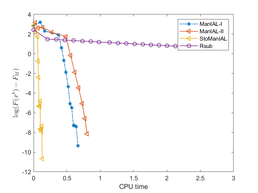
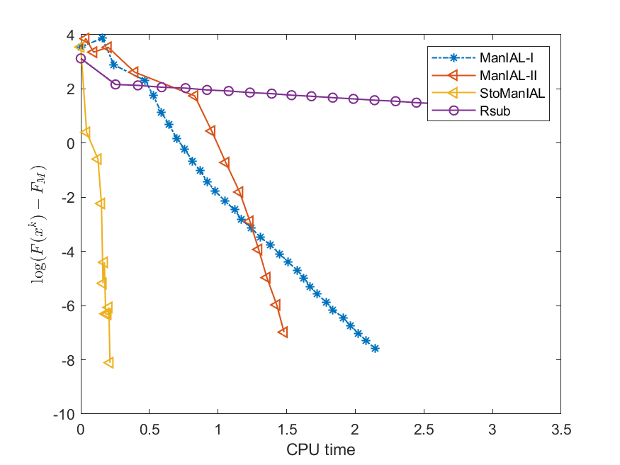
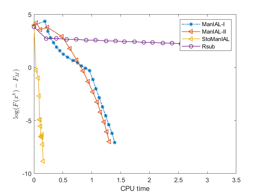
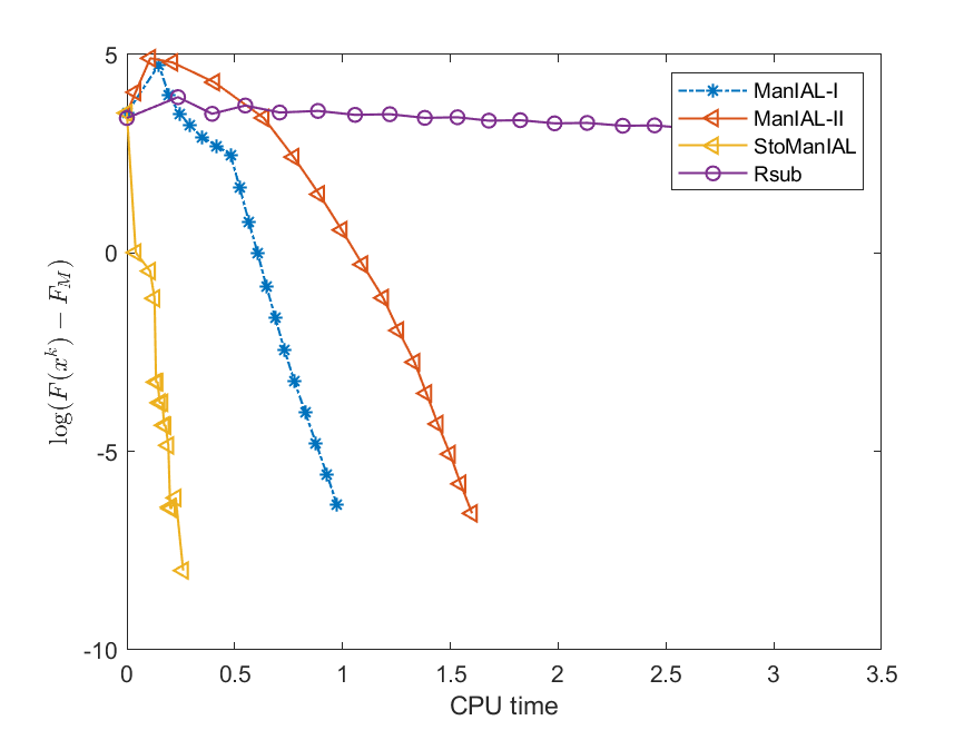
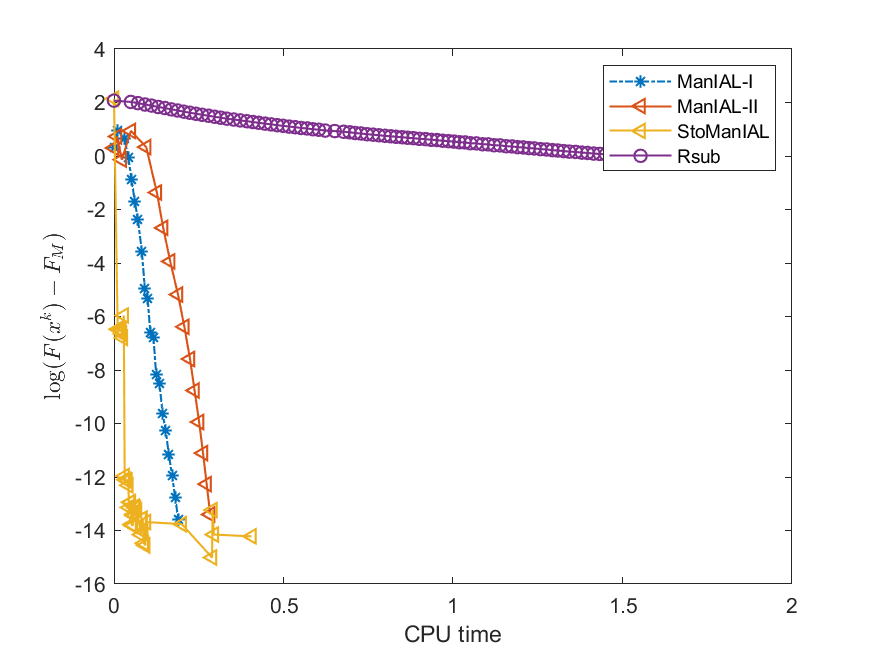
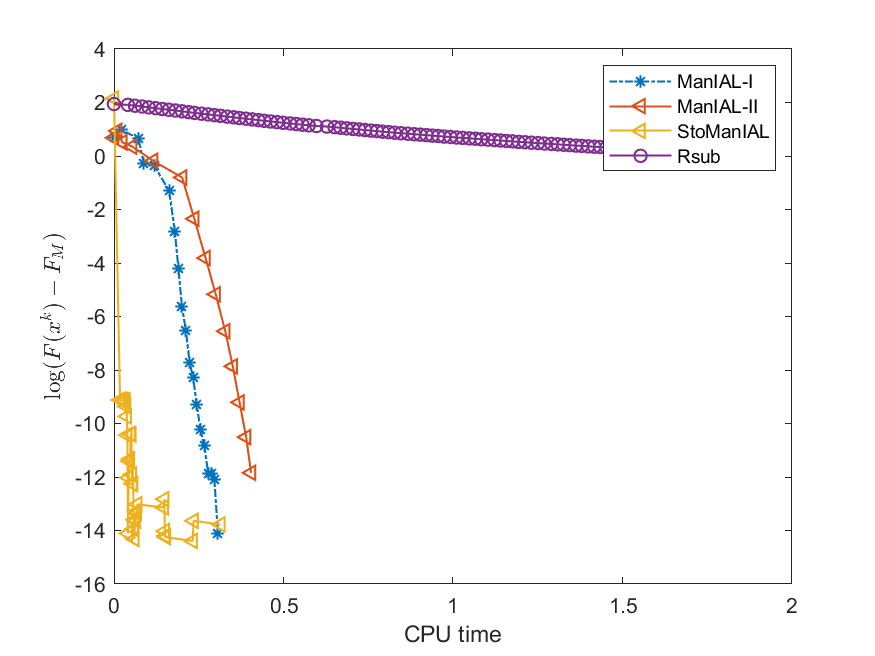
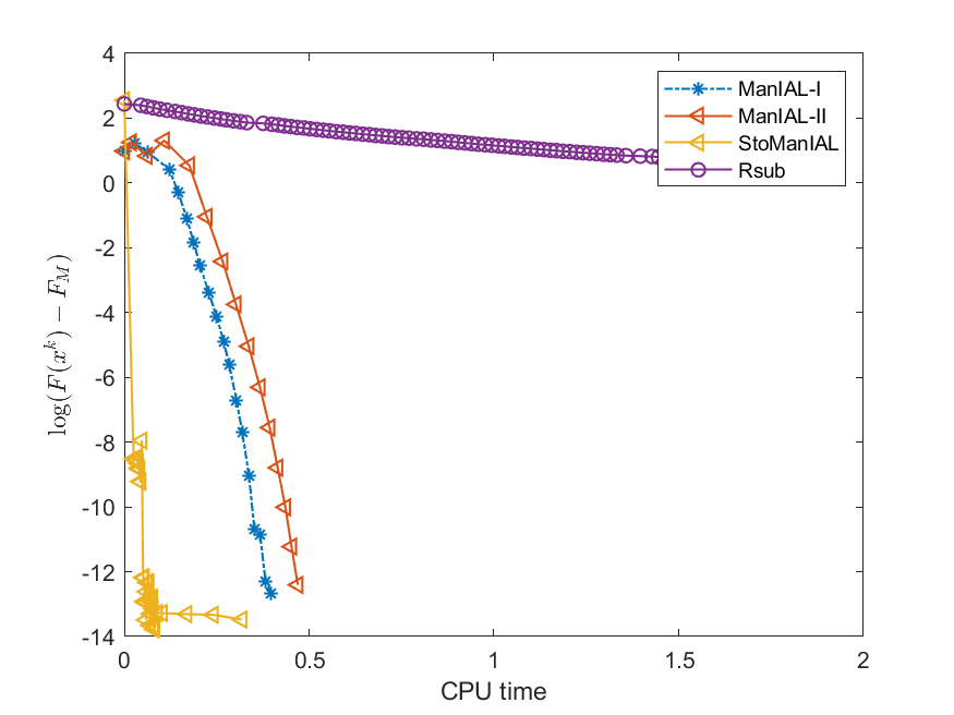
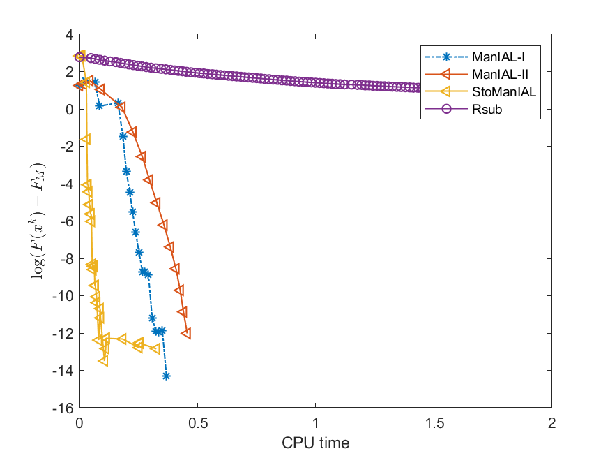
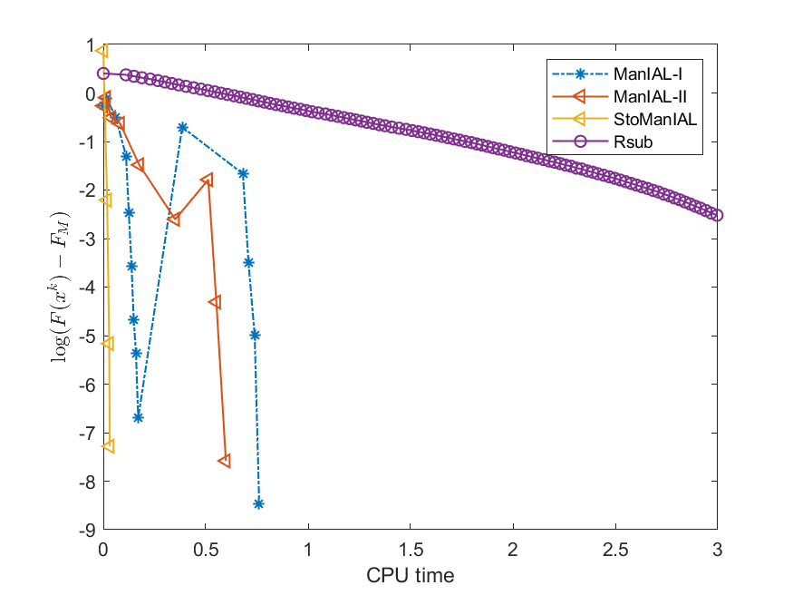
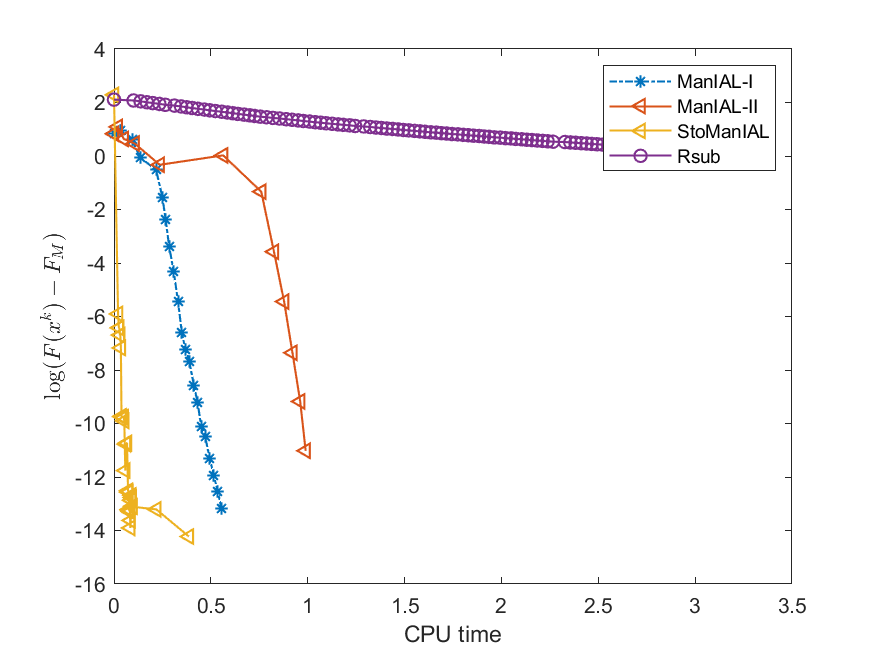
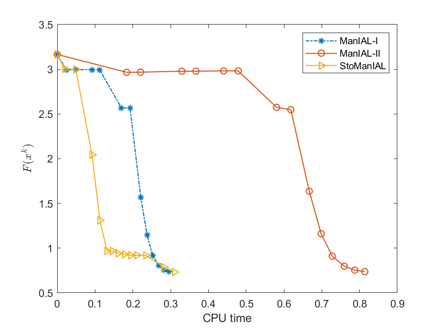
We first compare the performance of the proposed algorithms on the SPCA problem with random data, i.e., we set . For the StoManIAL, we partition the 50,000 samples into 100 subsets, and in each iteration, we sample one subset. The tolerance is set . Figure 1 presents the results of the four algorithms for fixed and varying and . The horizontal axis represents CPU time, while the vertical axis represents the objective function value gap: , where is given by the ManIAL-I. The results indicate that StoManIAL outperforms the deterministic version. Moreover, among the deterministic versions, ManIAL-I and ManIAL-II have similar performance. In conclusion, compared with the Rsub, our algorithms achieve better performance.
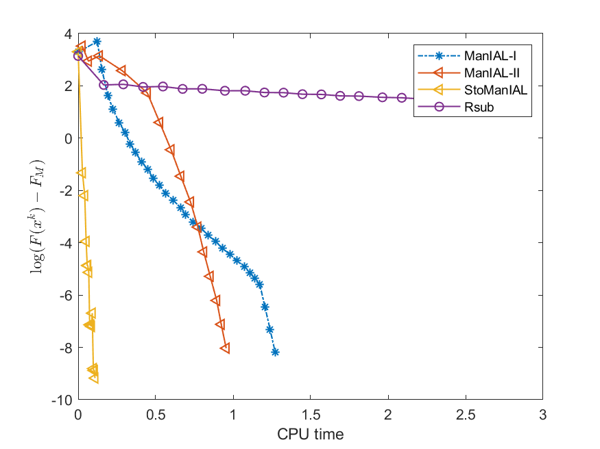
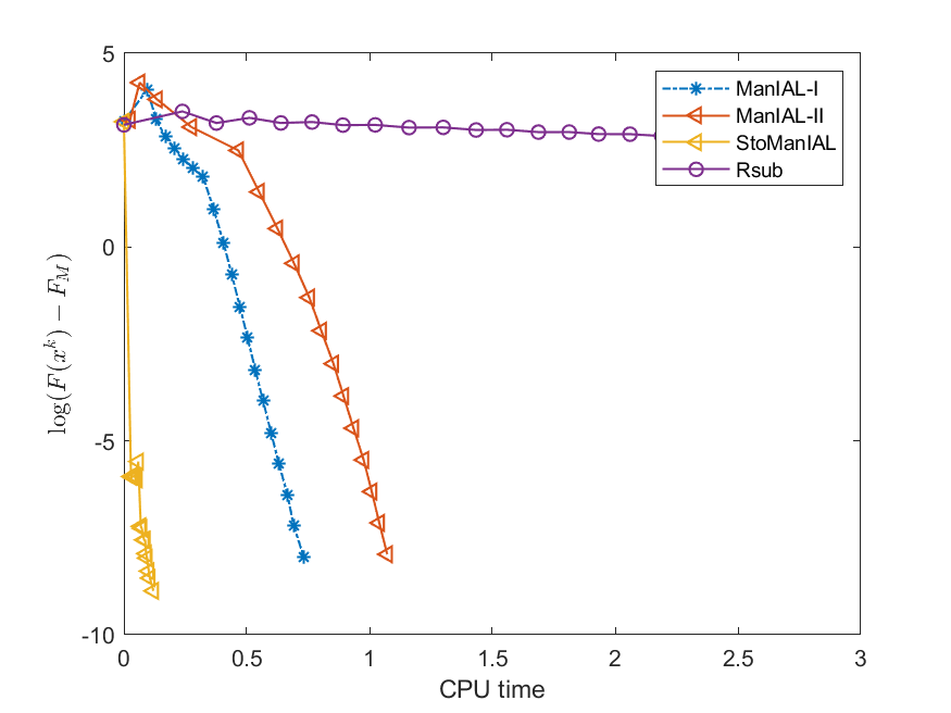
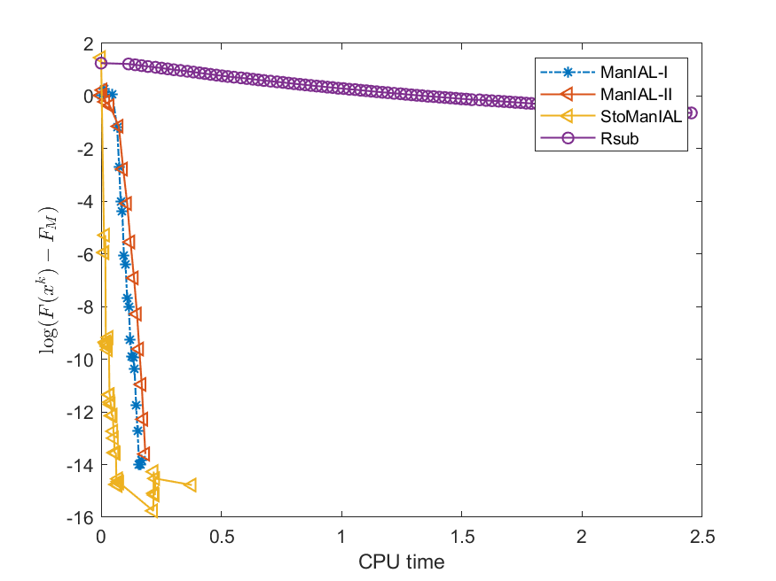
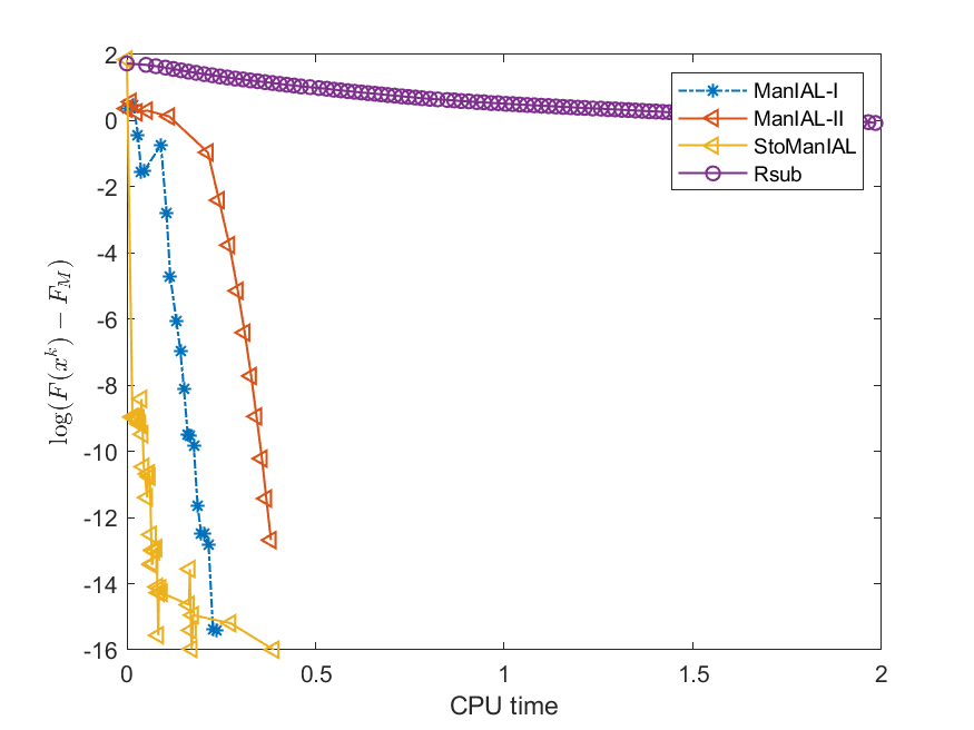
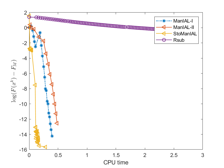
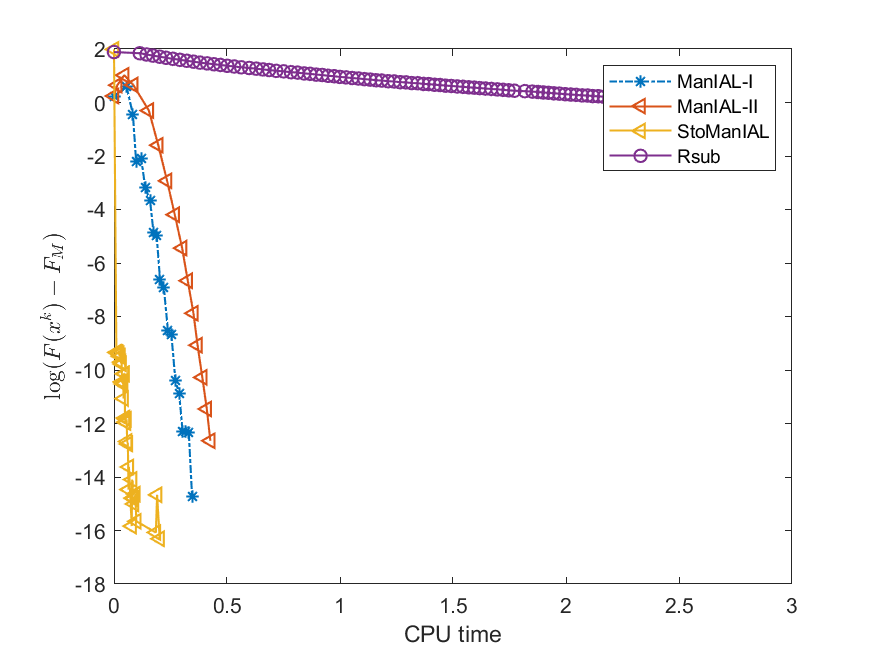
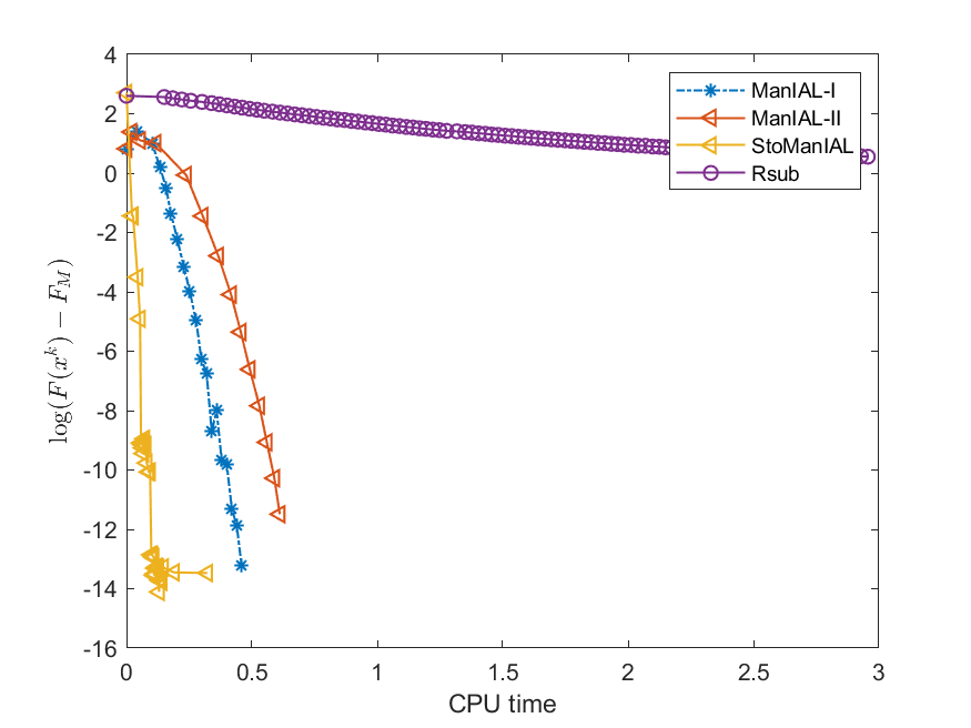
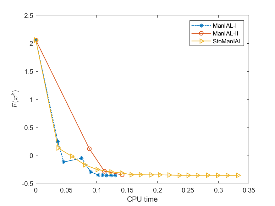
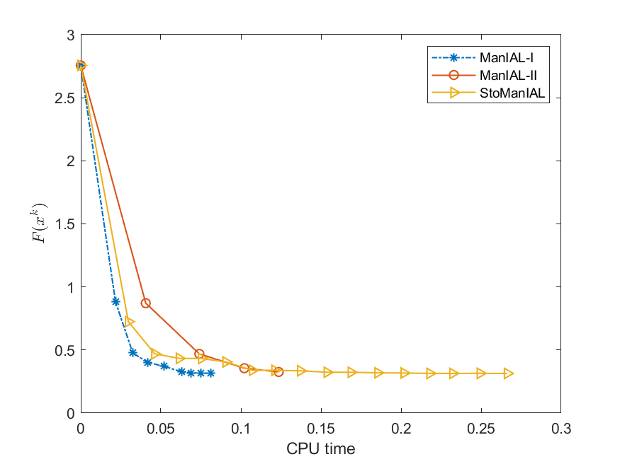
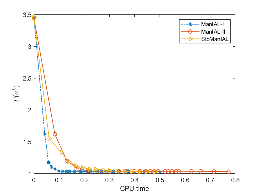
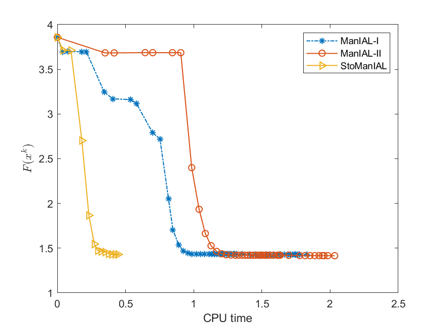
Next, we conduct experiments on two real datasets: coil100 [36] and mnist [28]. The coil100 dataset contains RGB images of 100 objects taken from different angles. The mnist dataset has grayscale digit images of size . Our experiments, illustrated in Figures 2 and 3, demonstrate that our algorithms outperform Rsub.
5.2 Sparse canonical correlation analysis
Canonical correlation analysis (CCA) first proposed by Hotelling [20] aims to tackle the associations between two sets of variables. The sparse CCA (SCCA) model is proposed to improve the interpretability of canonical variables by restricting the linear combinations to a subset of original variables. Suppose that there are two data sets: containing variables and containing variables, both are obtained from observations. Let be the sample covariance matrices of and , respectively, and be the sample cross-covariance matrix, then the SCCA can be formulated as
| (5.5) |
Let us denote and . Without loss of generality, we assume that and are positive definite (otherwise, we can impose a small identity matrix). In this case, and are two generalized Stiefel manifolds, problem (5.5) is a nonsmooth problem on a product manifold . Moreover, since , where denote the -th row of and , respectively, we can rewrite (5.5) as the following finite-sum form:
| (5.6) |
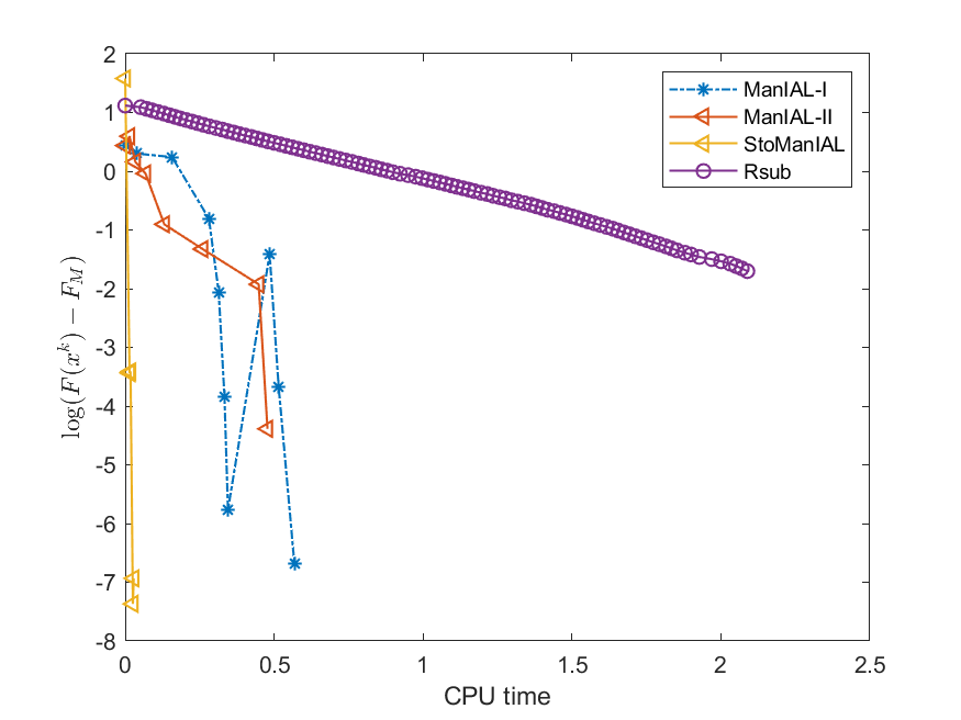
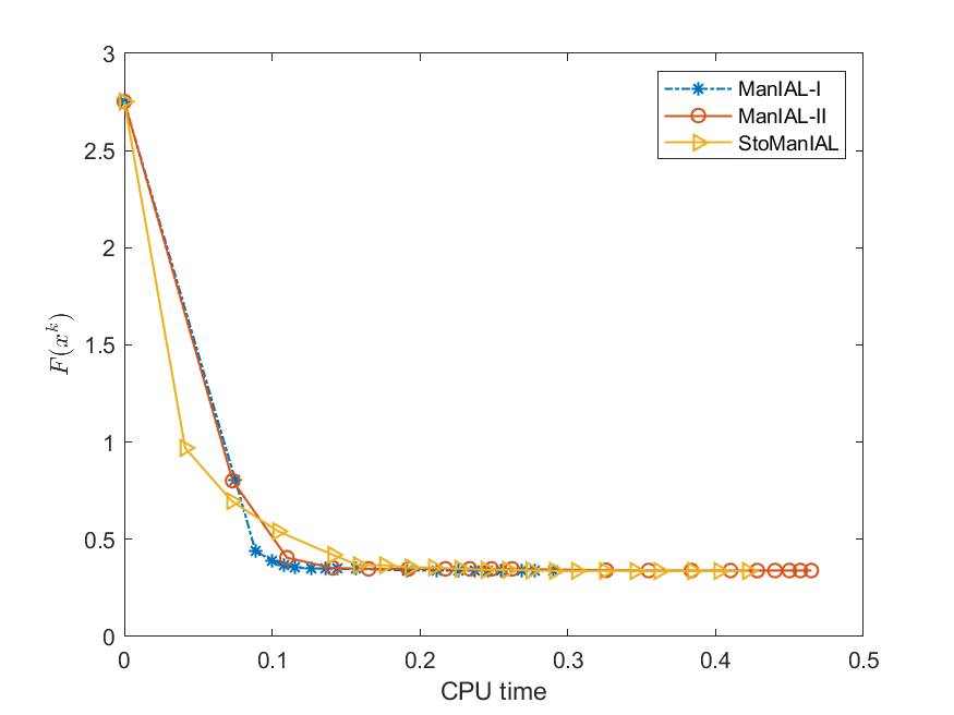
Therefore, we can apply our algorithms ManIAL and StoManIAL to solve (5.6). Owing to the poor performance in the SPCA problem, we only list the numerical comparisons of our algorithms. We compare the performance of the proposed algorithms on the SPCA problem with random data, i.e., we set . For the StoManIAL, we partition the 50,000 samples into 100 subsets, and in each iteration, we sample one subset. The tolerance is set . Figure 1 presents the results of the four algorithms for fixed and varying and . The results show that all algorithms have similar performance.
6 Conclusions
This paper proposes two novel manifold inexact augmented Lagrangian methods, namely ManIAL and StoManIAL, with the oracle complexity guarantee. To the best of our knowledge, this is the first complexity result for the augmented Lagrangian method for solving nonsmooth problems on Riemannian manifolds. We prove that ManIAL and StoManIAL achieve the oracle complexity of and , respectively. Numerical experiments on SPCA and SCCA problems demonstrate that our proposed methods outperform an existing method with the previously best-known complexity result.
References
- [1] P.-A. Absil, R. Mahony, and R. Sepulchre, Optimization Algorithms on Matrix Manifolds, Princeton University Press, Princeton, NJ, 2008.
- [2] N. Aybat and G. Iyengar, A first-order augmented Lagrangian method for compressed sensing, SIAM Journal on Optimization, 22 (2012), p. 429.
- [3] A. Beck and I. Rosset, A dynamic smoothing technique for a class of nonsmooth optimization problems on manifolds, SIAM Journal on Optimization, 33 (2023), pp. 1473–1493, https://doi.org/10.1137/22M1489447.
- [4] G. C. Bento, O. P. Ferreira, and J. G. Melo, Iteration-complexity of gradient, subgradient and proximal point methods on Riemannian manifolds, Journal of Optimization Theory and Applications, 173 (2017), pp. 548–562.
- [5] A. Böhm and S. J. Wright, Variable smoothing for weakly convex composite functions, Journal of optimization theory and applications, 188 (2021), pp. 628–649.
- [6] N. Boumal, An introduction to optimization on smooth manifolds, Cambridge University Press, Cambridge, England, 2023, https://doi.org/10.1017/9781009166164.
- [7] N. Boumal, P.-A. Absil, and C. Cartis, Global rates of convergence for nonconvex optimization on manifolds, IMA Journal of Numerical Analysis, 39 (2019), pp. 1–33.
- [8] S. Burer and R. D. Monteiro, A nonlinear programming algorithm for solving semidefinite programs via low-rank factorization, Mathematical programming, 95 (2003), pp. 329–357.
- [9] Y. Carmon, J. C. Duchi, O. Hinder, and A. Sidford, Accelerated methods for nonconvex optimization, SIAM Journal on Optimization, 28 (2018), pp. 1751–1772.
- [10] S. Chen, S. Ma, A. Man-Cho So, and T. Zhang, Proximal gradient method for nonsmooth optimization over the Siefel manifold, SIAM Journal on Optimization, 30 (2020), pp. 210–239.
- [11] A. Cutkosky and F. Orabona, Momentum-based variance reduction in non-convex sgd, Advances in neural information processing systems, 32 (2019).
- [12] K. Deng and Z. Peng, A manifold inexact augmented Lagrangian method for nonsmooth optimization on Riemannian submanifolds in Euclidean space, IMA Journal of Numerical Analysis, (2022), https://doi.org/10.1093/imanum/drac018.
- [13] Z. Deng, K. Deng, J. Hu, and Z. Wen, An augmented Lagrangian primal-dual semismooth newton method for multi-block composite optimization, arXiv preprint arXiv:2312.01273, (2023).
- [14] O. Ferreira and P. Oliveira, Subgradient algorithm on Riemannian manifolds, Journal of Optimization Theory and Applications, 97 (1998), pp. 93–104.
- [15] O. P. Ferreira, M. S. Louzeiro, and L. Prudente, Iteration-complexity of the subgradient method on Riemannian manifolds with lower bounded curvature, Optimization, 68 (2019), pp. 713–729.
- [16] S. Ghadimi and G. Lan, Accelerated gradient methods for nonconvex nonlinear and stochastic programming, Mathematical Programming, 156 (2016), pp. 59–99.
- [17] A. Han and J. Gao, Riemannian stochastic recursive momentum method for non-convex optimization, arXiv preprint arXiv:2008.04555, (2020).
- [18] S. Hosseini, W. Huang, and R. Yousefpour, Line search algorithms for locally Lipschitz functions on Riemannian manifolds, SIAM Journal on Optimization, 28 (2018), pp. 596–619.
- [19] S. Hosseini and A. Uschmajew, A Riemannian gradient sampling algorithm for nonsmooth optimization on manifolds, SIAM Journal on Optimization, 27 (2017), pp. 173–189.
- [20] H. Hotelling, Relations between two sets of variates, in Breakthroughs in statistics: methodology and distribution, Springer, 1992, pp. 162–190.
- [21] J. Hu, X. Liu, Z.-W. Wen, and Y.-X. Yuan, A brief introduction to manifold optimization, Journal of the Operations Research Society of China, 8 (2020), pp. 199–248.
- [22] W. Huang and K. Wei, Riemannian proximal gradient methods, Mathematical Programming, 194 (2022), pp. 371–413.
- [23] W. Huang and K. Wei, An inexact Riemannian proximal gradient method, Computational Optimization and Applications, 85 (2023), pp. 1–32.
- [24] B. Jiang, X. Meng, Z. Wen, and X. Chen, An exact penalty approach for optimization with nonnegative orthogonality constraints, Mathematical Programming, 198 (2023), pp. 855–897.
- [25] I. T. Jolliffe, N. T. Trendafilov, and M. Uddin, A modified principal component technique based on the LASSO, Journal of computational and Graphical Statistics, 12 (2003), pp. 531–547.
- [26] W. Kong, J. G. Melo, and R. D. Monteiro, Complexity of a quadratic penalty accelerated inexact proximal point method for solving linearly constrained nonconvex composite programs, SIAM Journal on Optimization, 29 (2019), pp. 2566–2593.
- [27] G. Lan and R. D. Monteiro, Iteration-complexity of first-order augmented Lagrangian methods for convex programming, Mathematical Programming, 155 (2016), pp. 511–547.
- [28] Y. LeCun, The mnist database of handwritten digits, http://yann. lecun. com/exdb/mnist/, (1998).
- [29] J. Li, S. Ma, and T. Srivastava, A Riemannian ADMM, arXiv preprint arXiv:2211.02163, (2022).
- [30] X. Li, S. Chen, Z. Deng, Q. Qu, Z. Zhu, and A. Man-Cho So, Weakly convex optimization over Stiefel manifold using Riemannian subgradient-type methods, SIAM Journal on Optimization, 31 (2021), pp. 1605–1634.
- [31] X. Li, D. Sun, and K.-C. Toh, A highly efficient semismooth Newton augmented Lagrangian method for solving lasso problems, SIAM Journal on Optimization, 28 (2018), pp. 433–458.
- [32] Z. Li, P.-Y. Chen, S. Liu, S. Lu, and Y. Xu, Rate-improved inexact augmented Lagrangian method for constrained nonconvex optimization, in International Conference on Artificial Intelligence and Statistics, PMLR, 2021, pp. 2170–2178.
- [33] Z. Li, P.-Y. Chen, S. Liu, S. Lu, and Y. Xu, Stochastic inexact augmented Lagrangian method for nonconvex expectation constrained optimization, Computational Optimization and Applications, 87 (2024), pp. 117–147.
- [34] Q. Lin, R. Ma, and Y. Xu, Inexact proximal-point penalty methods for constrained non-convex optimization, arXiv preprint arXiv:1908.11518, (2019).
- [35] Z. Lu and Z. Zhou, Iteration-complexity of first-order augmented Lagrangian methods for convex conic programming, SIAM journal on optimization, 33 (2023), pp. 1159–1190.
- [36] S. A. Nene, S. K. Nayar, H. Murase, et al., Columbia object image library (coil-20), (1996).
- [37] Z. Peng, W. Wu, J. Hu, and K. Deng, Riemannian smoothing gradient type algorithms for nonsmooth optimization problem on compact Riemannian submanifold embedded in Euclidean space, Applied Mathematics & Optimization, 88 (2023), p. 85.
- [38] M. F. Sahin, A. Eftekhari, A. Alacaoglu, F. L. Gómez, and V. Cevher, An inexact augmented Lagrangian framework for nonconvex optimization with nonlinear constraints, in Proceedings of NeurIPS 2019, 2019.
- [39] H. Sato, Riemannian optimization and its applications, Springer Cham, Cham, 2021, https://doi.org/doi.org/10.1007/978-3-030-62391-3.
- [40] B. Wang, S. Ma, and L. Xue, Riemannian stochastic proximal gradient methods for nonsmooth optimization over the Stiefel manifold, Journal of machine learning research, 23 (2022), pp. 1–33.
- [41] Y. Wang, K. Deng, H. Liu, and Z. Wen, A decomposition augmented Lagrangian method for low-rank semidefinite programming, SIAM Journal on Optimization, 33 (2023), pp. 1361–1390.
- [42] Y. Xu, First-order methods for constrained convex programming based on linearized augmented Lagrangian function, INFORMS Journal on Optimization, 3 (2021), pp. 89–117.
- [43] Y. Xu, Iteration complexity of inexact augmented Lagrangian methods for constrained convex programming, Mathematical Programming, 185 (2021), pp. 199–244.
- [44] R. Zass and A. Shashua, Nonnegative sparse PCA, Advances in neural information processing systems, 19 (2006).
- [45] J. Zhang, H. Lin, S. Jegelka, S. Sra, and A. Jadbabaie, Complexity of finding stationary points of nonconvex nonsmooth functions, in International Conference on Machine Learning, PMLR, 2020, pp. 11173–11182.
- [46] Y. Zhou, C. Bao, C. Ding, and J. Zhu, A semismooth Newton based augmented Lagrangian method for nonsmooth optimization on matrix manifolds, Mathematical Programming, (2022), pp. 1–61.
Appendix A Technical lemmas
The next lemma is a technical observation and follows from Lemma 3 in [11].
Proof A.3.
By retr-smoothness of , we have
where for the last inequality we choose .
The following technical lemma, which follows from Lemma 3 in [11], provides a recurrence variance bound.
Lemma A.4.
Appendix B The proof of Lemma 4.2
Proof B.1.
First, since , we have from the update formula of that . It follows from Lemma A.2 that
| (B.1) |
Consider the potential function . Since and , we have that for all
Then, we first consider . Using Lemma A.4, we obtain
Let us focus on the terms of this expression individually. For the first term, , observing that , we have
where in the second to last inequality we used Lemma 4 in [11]. For the second term , we have
Let us estimate . Using the concavity of , we have . Therefore:
where we use . Further, since , we have
Thus, we obtain . Putting all this together yields:
| (B.2) |
Now, we are ready to analyze the potential . It follows from (B.1) that
Summing over and using (B.2), we obtain
Reordering the terms, we have
where the last inequality is given by the definition of and in the algorithm. Now, we relate to . First, since is decreasing,
Therefore, if we set , to get
| (B.3) | ||||
It follows from (4.13) that
| (B.4) |
Plugging this in (B.3) and using we obtain:
where we have used the concavity of for all to move expectations inside the exponents. Now, define . Then the above can be rewritten as:
Note that this implies that either , or . Solving for in these two cases, we obtain
Finally, observe that by Cauchy-Schwarz we have so that
where we used in the last inequality.