Order Estimates for the Exact Lugannani–Rice Expansion

Takashi Kato ^*^**Division of Mathematical Science for Social Systems, Graduate School of Engineering Science, Osaka University, 1-3, Machikaneyama-cho, Toyonaka, Osaka 560-8531, Japan, E-mail: kato@sigmath.es.osaka-u.ac.jp Jun Sekine ^†^††Division of Mathematical Science for Social Systems, Graduate School of Engineering Science, Osaka University, 1-3, Machikaneyama-cho, Toyonaka, Osaka 560-8531, Japan, E-mail: sekine@sigmath.es.osaka-u.ac.jp Kenichi Yoshikawa ^‡^‡‡Sumitomo Mitsui Banking Corporation, E-mail: k.yoshi6208@gmail.com

(First version: October 12, 2013
This version: June 15, 2014)

Abstract

The Lugannani–Rice formula is a saddlepoint approximation method for estimating the tail probability distribution function, which was originally studied for the sum of independent identically distributed random variables. Because of its tractability, the formula is now widely used in practical financial engineering as an approximation formula for the distribution of a (single) random variable. In this paper, the Lugannani–Rice approximation formula is derived for a general, parametrized sequence $\displaystyle(X^{(\varepsilon)})_{\varepsilon>0}$ of random variables and the order estimates (as $\displaystyle\varepsilon\to 0$ ) of the approximation are given.

⁰⁰0Mathematical Subject Classification (2010) 62E17, 91G60, 65D15
⁰⁰0JEL Classification (2010) C63 , C65

Keywords: Saddlepoint approximation, The Lugannani–Rice formula, Order estimates, Asymptotic expansion, Stochastic volatility models

1 Introduction

Saddlepoint approximations (SPAs) provide effective methods for approximating probability density functions and tail probability distribution functions, using their cumulant generating functions (CGFs). In mathematical statistics, SPA methods originated with Daniels (1954), in which an approximation formula was given for the density function of the sample mean $\displaystyle\bar{X}_{n}=(X_{1}+\cdots+X_{n})/n$ of independent identically distributed (i.i.d.) random variables $\displaystyle(X_{i})_{i\in{\mathbb{N}}}$ , provided that the law of $\displaystyle X_{1}$ has the density function. Lugannani and Rice (1980) derives the following approximation formula for the right tail probability:

P(\bar{X}_{n}>x)=1-\Phi(\hat{w}_{n})+\phi(\hat{w}_{n})\left(\frac{1}{\hat{u}_{n}}-\frac{1}{\hat{w}_{n}}\right)+O(n^{-3/2})

(1.1)

as $\displaystyle n\to\infty$ . Here, $\displaystyle\Phi(w)$ and $\displaystyle\phi(w)$ are the standard normal distribution function and its density function $\displaystyle\phi:=\Phi^{\prime}$ , respectively, and $\displaystyle\hat{u}_{n}$ and $\displaystyle\hat{w}_{n}$ are expressed by using the CGF $\displaystyle K(\cdot)$ of $\displaystyle X_{1}$ and the saddlepoint $\displaystyle\hat{\theta}$ of $\displaystyle K(\cdot)$ . That is, $\displaystyle\hat{\theta}$ satisfies $\displaystyle K^{\prime}(\hat{\theta})=x$ . Related SPA formulae have been studied in Daniels (1987), Jensen (1995), Kolassa (1997), Butler (2007), the references therein, and others.

Strictly, the Lugannani–Rice (LR) formula (1.1) should be interpreted as an asymptotic result as $\displaystyle n\rightarrow\infty$ . However, it is popular in many practical applications of financial engineering as an approximation formula for the right tail probability because of its tractability. This approximation is

\displaystyle\displaystyle P(X_{1}>x)\approx 1-\Phi(\hat{w}_{1})+\phi(\hat{w}_{1})\left(\frac{1}{\hat{u}_{1}}-\frac{1}{\hat{w}_{1}}\right).

(1.2)

In other words, LR formula (1.1) is applied even when $\displaystyle n$ is $\displaystyle 1$ ! For financial applications of SPA formulae, we refer the readers to papers such as Rogers and Zane (1999), Xiong, Wong, and Salopek (2005), Aït-Sahalia and Yu (2006), Yang, Hurd, and Zhang (2006), Glasserman and Kim (2009), and Carr and Madan (2009). It is interesting that the approximation formula (1.2) still works surprisingly well in many financial examples, despite its lack of theoretical justification.

The aim of this paper is to provide a measure of the effectivity of the “generalized usage” of the LR formula (1.2) from an asymptotic theoretical viewpoint. We consider a general parametrized sequence of random variables $\displaystyle(X^{(\varepsilon)})_{\varepsilon>0}$ and assume that the $\displaystyle r$ th cumulant of $\displaystyle X^{(\varepsilon)}$ has order $\displaystyle O(\varepsilon^{r-2})$ as $\displaystyle\varepsilon\rightarrow 0$ for each $\displaystyle r\geq 3$ . This implies that $\displaystyle X^{(\varepsilon)}$ converges in law to a normally distributed random variable (a motivation is provided for this assumption in Remark 2 of Section 3). We next derive the expansion

P\left(X^{(\varepsilon)}>x\right)=1-\Phi(\hat{w}_{\varepsilon})+\sum^{\infty}_{m=0}\Psi^{\varepsilon}_{m}(\hat{w}_{\varepsilon}),

(1.3)

which we call the exact LR expansion (see Theorem 1 of Section 2). Here, $\displaystyle\hat{w}_{\varepsilon}$ is given by (2.1) and (2.3), and the $\displaystyle\Psi^{\varepsilon}_{m}(\hat{w}_{\varepsilon})$ ( $\displaystyle m\in{\mathbb{Z}}_{+}$ ) are given by (2.8). We then show that

\displaystyle\Psi^{\varepsilon}_{0}(\hat{w}_{\varepsilon})=O(\varepsilon)

and

\displaystyle\Psi^{\varepsilon}_{m}(\hat{w}_{\varepsilon})=O(\varepsilon^{3})

\displaystyle\varepsilon\rightarrow 0

for all

\displaystyle m\in{\mathbb{N}}

(1.4)

under some conditions. This is the main result of the paper (see Theorem 2 in Section 3 for the details).

Remark 1.

We note that the expansion (1.3) with the order estimates (1.4) and the classical LR formula (1.1) treat different situations, although they may have some overlap. Let

\displaystyle\displaystyle\varepsilon:=\frac{1}{\sqrt{N}}\quad\text{and}\quad X^{(\varepsilon)}:=\varepsilon\sum_{i=1}^{1/\varepsilon^{2}}X_{i},

where $\displaystyle(X_{i})_{i\in{\mathbb{N}}}$ is an i.i.d. sequence of random variables. Then, we can check that the law of $\displaystyle X^{(\varepsilon)}$ satisfies the conditions necessary to apply Theorem 2 in Section 3 (see Remark 2 (iv) in Section 3). So, (1.3) holds with (1.4). On the other hand, the classical LR formula (1.1) gives an approximation formula of the far-right tail probability:

\displaystyle\displaystyle P\left({X}^{(\varepsilon)}>\frac{x}{\varepsilon}\right)=1-\Phi(\hat{w}_{\varepsilon})+\phi(\hat{w}_{\varepsilon})\left(\frac{1}{\hat{u}_{\varepsilon}}-\frac{1}{\hat{w}_{\varepsilon}}\right)+O(\varepsilon^{3})\ \ \mbox{as}\ \ \varepsilon\rightarrow 0.

In this paper, with motivation from financial applications (e.g., call option pricing in Section 4), we choose to analyse the right tail probability $\displaystyle P(X^{(\varepsilon)}>x)$ instead of the far-right tail probability $\displaystyle P(X^{(\varepsilon)}>x/\varepsilon)$ . For a related remark, see (i) in Section 7.

The organisation of the rest of this paper is as follows. In Section 2, we introduce the “exact” LR expansion: we first derive it formally, and next provide a technical condition sufficient to ensure the validity of the expansion. Section 3 states our main results: we derive the order estimates of the higher order terms in the exact LR expansion (1.3). Section 4 discusses some examples: we introduce two stochastic volatility (SV) models and numerically check the accuracy of the higher order LR formula. Section 5 contains the necessary proofs: Subsection 5.1 gives the proof of Theorem 1 and Subsection 5.2 gives the proof of Theorem 2. Section 6 discusses some extensions of Theorem 2: under additional conditions we obtain the sharper estimate $\displaystyle\Psi^{\varepsilon}_{m}(\hat{w}_{\varepsilon})=O(\varepsilon^{2m+1})$ as $\displaystyle\varepsilon\rightarrow 0$ for $\displaystyle m\in{\mathbb{N}}$ , and the related order estimate of the absolute error of the $\displaystyle M$ th order LR formula. In addition, we introduce error estimates for the Daniels-type formula, which is an approximation formula for the probability density function. The last Section 7 contains concluding remarks. In Appendix, we present some toolkits for deriving the explicit forms of $\displaystyle\Psi^{\varepsilon}_{2}(\hat{w}_{\varepsilon})$ and $\displaystyle\Psi^{\varepsilon}_{3}(\hat{w}_{\varepsilon})$ .

2 The Exact Lugannani–Rice Expansion

In this section we derive the exact LR expansion (1.3), which is given as a natural generalisation of the original LR formula. For readability, we introduce here the formal calculations to derive that formula and leave rigorous arguments to Section 5.1 (see also Appendix in Rogers and Zane (1999)).

Let $\displaystyle(\mu_{\varepsilon})_{0\leq\varepsilon\leq 1}$ be a family of probability distribution on $\displaystyle\mathbb{R}$ and define a distribution function $\displaystyle F_{\varepsilon}$ and a tail probability function $\displaystyle\bar{F}_{\varepsilon}$ by

\displaystyle\displaystyle F_{\varepsilon}(x)=\mu_{\varepsilon}((-\infty,x]),\ \ \bar{F}_{\varepsilon}(x)=1-F_{\varepsilon}(x).

We denote by $\displaystyle K_{\varepsilon}$ the CGF of $\displaystyle\mu_{\varepsilon}$ , that is,

\displaystyle\displaystyle K_{\varepsilon}(\theta)=\log\int_{\mathbb{R}}e^{\theta x}\mu_{\varepsilon}(dx).

We assume the following conditions.

[A1]

For each $\displaystyle\varepsilon\in[0,1]$ , the effective domain $\displaystyle\mathcal{D}_{\varepsilon}=\{\theta\in\mathbb{R}\ ;\ |K_{\varepsilon}(\theta)|<\infty\}$ of $\displaystyle K_{\varepsilon}$ contains an open interval that includes zero.

[A2]

For each $\displaystyle\varepsilon\in[0,1]$ , the support of $\displaystyle\mu_{\varepsilon}$ is equal to the whole line $\displaystyle\mathbb{R}$ . Moreover, the characteristic function of $\displaystyle\mu_{\varepsilon}$ is integrable; that is,

\displaystyle\displaystyle\int^{\infty}_{-\infty}\left|\int^{\infty}_{-\infty}e^{i\xi x}\mu_{\varepsilon}(dx)\right|d\xi<\infty,

where $\displaystyle i=\sqrt{-1}$ is the imaginary unit.

It is well known that $\displaystyle K_{\varepsilon}$ is analytic and convex on the interior $\displaystyle\mathcal{O}_{\varepsilon}$ of $\displaystyle\mathcal{D}_{\varepsilon}$ . Moreover, [A2] implies that $\displaystyle\mu_{\varepsilon}$ has a density function, and thus $\displaystyle K_{\varepsilon}$ is a strictly convex function (see Durrett (2010), for instance). Since the range of $\displaystyle K^{\prime}_{\varepsilon}$ coincides with $\displaystyle\mathbb{R}$ under [A1]–[A2], we can always find the solution $\displaystyle\hat{\theta}_{\varepsilon}=\hat{\theta}_{\varepsilon}(x)\in\mathcal{O}_{\varepsilon}$ to

\displaystyle\displaystyle K^{\prime}_{\varepsilon}(\hat{\theta}_{\varepsilon})=x

(2.1)

for any $\displaystyle x\in\mathbb{R}$ . We call $\displaystyle\hat{\theta}_{\varepsilon}$ the saddlepoint of $\displaystyle K_{\varepsilon}$ given $\displaystyle x$ . Here, note that $\displaystyle K_{\varepsilon}$ is analytically continued as the function defined on $\displaystyle\mathcal{O}_{\varepsilon}\times i\mathbb{R}$ .

Now, we derive (1.3). Until the end of this section, we fix an $\displaystyle\varepsilon\in[0,1]$ and an $\displaystyle x\in\mathbb{R}$ . To derive (1.3), we further that require the condition $\displaystyle\hat{\theta}_{\varepsilon}\neq 0$ be satisfied. Applying Levy’s inversion formula, we represent $\displaystyle\bar{F}_{\varepsilon}(x)$ by the integral form

\displaystyle\displaystyle\bar{F}_{\varepsilon}(x)\ =\ \frac{1}{2\pi i}\int^{c+i\infty}_{c-i\infty}\exp(K_{\varepsilon}(\theta)-x\theta)\frac{d\theta}{\theta}

(2.2)

for arbitrary $\displaystyle c\in\mathcal{O}_{\varepsilon}\setminus\{0\}$ (see Proposition 1 in Subsection 5.1).

Next, we represent $\displaystyle\hat{w}_{\varepsilon}\in\mathbb{R}$ as

\displaystyle\displaystyle\hat{w}_{\varepsilon}=\mathrm{sgn}(\hat{\theta}_{\varepsilon})\sqrt{2(x\hat{\theta}_{\varepsilon}-K_{\varepsilon}(\hat{\theta}_{\varepsilon}))},

(2.3)

where $\displaystyle\mathrm{sgn}(a)=1\ (a\geq 0),\ -1\ (a<0)$ . Note that $\displaystyle\hat{w}_{\varepsilon}$ is well defined because of the calculation

	$\displaystyle\displaystyle x\hat{\theta}_{\varepsilon}-K_{\varepsilon}(\hat{\theta}_{\varepsilon})$	$\displaystyle\displaystyle=$	$\displaystyle\displaystyle K_{\varepsilon}(0)-K_{\varepsilon}(\hat{\theta}_{\varepsilon})+K^{\prime}_{\varepsilon}(\hat{\theta}_{\varepsilon})\hat{\theta}_{\varepsilon}$		(2.4)
		$\displaystyle\displaystyle=$	$\displaystyle\displaystyle\int^{1}_{0}(1-u)K^{\prime\prime}_{\varepsilon}(-u\hat{\theta}_{\varepsilon})du\hat{\theta}_{\varepsilon}^{2}\ \geq\ 0$		(2.4)

by virtue of the convexity of $\displaystyle K_{\varepsilon}$ and Taylor’s theorem. We consider the following change of variables between $\displaystyle w$ and $\displaystyle\theta$ :

\displaystyle\displaystyle\frac{1}{2}w^{2}-\hat{w}_{\varepsilon}w=K_{\varepsilon}(\theta)-x\theta.

(2.5)

Then, replacing the variable $\displaystyle\theta$ with $\displaystyle w$ in the right-hand side of (2.2) and applying Cauchy’s integral theorem, we see that

	$\displaystyle\displaystyle\bar{F}_{\varepsilon}(x)$	$\displaystyle\displaystyle=$	$\displaystyle\displaystyle\frac{1}{2\pi i}\int_{\gamma_{\varepsilon}}\exp\left(\frac{1}{2}w^{2}-\hat{w}_{\varepsilon}w\right)\frac{\theta^{\prime}(w)}{\theta(w)}dw$		(2.6)
		$\displaystyle\displaystyle=$	$\displaystyle\displaystyle\frac{1}{2\pi i}\int^{\hat{w}_{\varepsilon}+i\infty}_{\hat{w}_{\varepsilon}-i\infty}\exp\left(\frac{1}{2}w^{2}-\hat{w}_{\varepsilon}w\right)\frac{\theta^{\prime}(w)}{\theta(w)}dw,$		(2.6)

where $\displaystyle\gamma_{\varepsilon}$ is a Jordan curve in $\displaystyle w$ -space corresponding to the line $\displaystyle\{\hat{\theta}_{\varepsilon}\}\times i\mathbb{R}$ and $\displaystyle\theta(w)\ (=\theta_{\varepsilon}(w))$ is defined by (2.5) as an implicit function with respect to $\displaystyle w$ . Note that $\displaystyle\theta(w)$ is well defined for each $\displaystyle w$ and is analytic on each contour under suitable conditions. Denoting

\displaystyle\displaystyle\psi_{\varepsilon}(w)=\frac{\theta^{\prime}(w)}{\theta(w)}-\frac{1}{w}=\frac{d}{dw}\log\left(\frac{\theta(w)}{w}\right),

we can decompose (2.6) into

\displaystyle\displaystyle\bar{F}_{\varepsilon}(x)=N_{\varepsilon}(x)+\frac{1}{2\pi i}\int^{\hat{w}_{\varepsilon}+i\infty}_{\hat{w}_{\varepsilon}-i\infty}\exp\left(\frac{1}{2}w^{2}-\hat{w}_{\varepsilon}w\right)\psi_{\varepsilon}(w)dw,

where

\displaystyle\displaystyle N_{\varepsilon}(x)

\displaystyle\displaystyle=

\displaystyle\displaystyle\frac{1}{2\pi i}\int^{\hat{w}_{\varepsilon}+i\infty}_{\hat{w}_{\varepsilon}-i\infty}\exp\left(\frac{1}{2}w^{2}-\hat{w}_{\varepsilon}w\right)\frac{dw}{w}.

$\displaystyle N_{\varepsilon}(x)$ is just the tail probability of the standard normal distribution; that is, $\displaystyle N_{\varepsilon}(x)=\bar{\Phi}(\hat{w}_{\varepsilon})$ , where

\displaystyle\displaystyle\bar{\Phi}(w)\ =\ \int^{\infty}_{w}\phi(y)dy,\ \ \phi(y)\ =\ \frac{1}{\sqrt{2\pi}}e^{-y^{2}/2}.

Here, if $\displaystyle\hat{w}_{\varepsilon}\neq 0$ , we see that $\displaystyle\psi_{\varepsilon}$ is analytic on $\displaystyle\{\hat{w}_{\varepsilon}\}\times i\mathbb{R}$ ; hence, we obtain

	$\displaystyle\displaystyle\frac{1}{2\pi i}\int^{\hat{w}_{\varepsilon}+i\infty}_{\hat{w}_{\varepsilon}-i\infty}\exp\left(\frac{1}{2}w^{2}-\hat{w}_{\varepsilon}w\right)\psi_{\varepsilon}(w)dw$	(2.7)
$\displaystyle\displaystyle=$	$\displaystyle\displaystyle\frac{1}{2\pi i}\int^{\hat{w}_{\varepsilon}+i\infty}_{\hat{w}_{\varepsilon}-i\infty}\exp\left(\frac{1}{2}w^{2}-\hat{w}_{\varepsilon}w\right)\sum^{\infty}_{n=0}\frac{\psi_{\varepsilon}^{(n)}(\hat{w}_{\varepsilon})}{n!}(w-\hat{w}_{\varepsilon})^{n}dw$
$\displaystyle\displaystyle=$	$\displaystyle\displaystyle\frac{1}{2\pi}e^{-\hat{w}_{\varepsilon}^{2}/2}\int^{\infty}_{-\infty}e^{-y^{2}/2}\sum^{\infty}_{n=0}\frac{\psi_{\varepsilon}^{(n)}(\hat{w}_{\varepsilon})}{n!}(iy)^{n}dy$
$\displaystyle\displaystyle=$	$\displaystyle\displaystyle\frac{1}{2\pi}e^{-\hat{w}_{\varepsilon}^{2}/2}\sum^{\infty}_{n=0}i^{n}\psi_{\varepsilon}^{(n)}(\hat{w}_{\varepsilon})\int^{\infty}_{-\infty}e^{-y^{2}/2}\frac{y^{n}}{n!}dy\ =\ \sum^{\infty}_{m=0}\Psi^{\varepsilon}_{m}(\hat{w}_{\varepsilon}),$

where we define

\Psi_{m}^{\varepsilon}(w)=\phi(w)\frac{(-1)^{m}}{(2m)!!}\psi^{(2m)}_{\varepsilon}(w)=\phi(w)\frac{(-1)^{m}}{(2m)(2m-2)\cdots 4\cdot 2}\psi^{(2m)}_{\varepsilon}(w).

(2.8)

This is the exact LR expansion (1.3). Note here that the $\displaystyle 0$ th order approximation formula

\displaystyle\displaystyle\bar{\Phi}(\hat{w}_{\varepsilon})+\Psi_{0}^{\varepsilon}(\hat{w}_{\varepsilon})

corresponds to the original LR formula (1.1). Indeed, we see that

\displaystyle\displaystyle\Psi_{0}^{\varepsilon}(\hat{w}_{\varepsilon})=\phi(\hat{w}_{\varepsilon})\left\{\frac{1}{\hat{\theta}_{\varepsilon}\sqrt{K^{\prime\prime}_{\varepsilon}(\hat{\theta}_{\varepsilon})}}-\frac{1}{\hat{w}_{\varepsilon}}\right\}.

The $\displaystyle 1$ st order approximation formula

\displaystyle\displaystyle\bar{\Phi}(\hat{w}_{\varepsilon})+\Psi^{\varepsilon}_{0}(\hat{w}_{\varepsilon})+\Psi^{\varepsilon}_{1}(\hat{w}_{\varepsilon})

is also often called the LR formula, where we have that

\displaystyle\displaystyle\Psi_{1}^{\varepsilon}(\hat{w}_{\varepsilon})=\phi(\hat{w}_{\varepsilon})\left\{\frac{1}{\hat{\theta}_{\varepsilon}\sqrt{K^{\prime\prime}_{\varepsilon}(\hat{\theta}_{\varepsilon})}}\left(\frac{1}{8}\hat{\lambda}_{4}-\frac{5}{24}\hat{\lambda}^{2}_{3}\right)-\frac{1}{2\hat{\theta}_{\varepsilon}^{2}K^{\prime\prime}_{\varepsilon}(\hat{\theta}_{\varepsilon})}\hat{\lambda}_{3}-\left(\frac{1}{\hat{\theta}_{\varepsilon}^{3}(K^{\prime\prime}_{\varepsilon}(\hat{\theta}_{\varepsilon}))^{3/2}}-\frac{1}{\hat{w}_{\varepsilon}^{3}}\right)\right\}

with

\displaystyle\displaystyle\hat{\lambda}_{3}=\frac{K^{(3)}_{\varepsilon}(\hat{\theta}_{\varepsilon})}{\left(K^{\prime\prime}_{\varepsilon}(\hat{\theta}_{\varepsilon})\right)^{3/2}},\ \ \hat{\lambda}_{4}=\frac{K^{(4)}_{\varepsilon}(\hat{\theta}_{\varepsilon})}{\left(K^{\prime\prime}_{\varepsilon}(\hat{\theta}_{\varepsilon})\right)^{2}}.

The explicit forms of the higher order terms $\displaystyle\Psi_{2}^{\varepsilon}(\hat{w}_{\varepsilon})$ and $\displaystyle\Psi_{3}^{\varepsilon}(\hat{w}_{\varepsilon})$ are shown in Appendix.

The above formal derivation of the exact LR expansion (1.3) can be made rigorous under suitable conditions, such as the following.

[B1]

For each $\displaystyle\varepsilon\in[0,1]$ , there exists $\displaystyle\delta_{\varepsilon},C_{\varepsilon}>0$ such that $\displaystyle\delta_{\varepsilon}\leq|K^{\prime\prime}_{\varepsilon}|\leq C_{\varepsilon}$ on $\displaystyle\mathcal{O}_{\varepsilon}\times i\mathbb{R}$ .

[B2]

The range of the holomorphic map $\displaystyle\iota_{\varepsilon}:\mathcal{O}_{\varepsilon}\times i\mathbb{R}\longrightarrow\mathbb{C}$ defined by

\displaystyle\displaystyle\iota_{\varepsilon}(\theta)=K_{\varepsilon}(\theta)-x\theta-(K_{\varepsilon}(\hat{\theta}_{\varepsilon})-x\hat{\theta}_{\varepsilon})

includes a convex set that contains $\displaystyle\{2\iota_{\varepsilon}(\hat{\theta}_{\varepsilon}+it)\ ;\ t\in\mathbb{R}\}$ and $\displaystyle(-\infty,0]$ ,

[B3]

$\displaystyle\sum^{\infty}_{n=1}|\psi_{\varepsilon}^{(n)}(\hat{w}_{\varepsilon})|/(n!!)<\infty$ .

Under these conditions, we obtain the following, whose proof is given in Subsection 5.1.

Theorem 1.

Assume $\displaystyle\mathrm{[A1]}$ – $\displaystyle\mathrm{[A2]}$ and $\displaystyle\mathrm{[B1]}$ – $\displaystyle\mathrm{[B3]}$ . Then $\displaystyle(\ref{exact_LR})$ holds.

3 Order Estimates of Approximation Terms

In practical applications, we need to truncate the formula (1.3) with $\displaystyle M\in{\mathbb{N}}$

\displaystyle\displaystyle\bar{F}_{\varepsilon}(x)\approx\bar{F}^{M}_{\varepsilon}(x):=\bar{\Phi}(\hat{w}_{\varepsilon})+\sum^{M}_{m=0}\Psi^{\varepsilon}_{m}(\hat{w}_{\varepsilon}).

(3.1)

We call the right-hand side of (3.1) the $\displaystyle M$ th LR formula. The aim of this section is to derive order estimates for $\displaystyle\Psi_{m}(\hat{w}_{\varepsilon})$ ( $\displaystyle m=0,1,\ldots,$ ) as $\displaystyle\varepsilon\rightarrow 0$ .

We fix $\displaystyle x\in\mathbb{R}$ , which is an arbitrary value such that

\int_{\mathbb{R}}y\mu_{0}(dy)\neq x.

(3.2)

We then impose the following additional assumptions.

[A3]

There is a $\displaystyle\delta_{0}>0$ such that $\displaystyle K^{\prime\prime}_{\varepsilon}(\theta)\geq\delta_{0}$ for each $\displaystyle\theta\in\mathcal{O}_{\varepsilon}$ and $\displaystyle\varepsilon\in[0,1]$ .
[A4]

For each $\displaystyle\varepsilon$ , there is an interval $\displaystyle\mathcal{I}_{\varepsilon}\subset\mathcal{D}_{\varepsilon}$ such that $\displaystyle\mathcal{I}_{\varepsilon}\nearrow\mathbb{R}$ as $\displaystyle\varepsilon\rightarrow 0$ ; that is, $\displaystyle\mathcal{I}_{\varepsilon}\subset\mathcal{I}_{\varepsilon^{\prime}}$ for each $\displaystyle\varepsilon\geq\varepsilon^{\prime}$ and $\displaystyle\cup_{\varepsilon}\mathcal{I}_{\varepsilon}=\mathbb{R}$ .

[A5]

For each nonnegative integer $\displaystyle r$ , $\displaystyle K^{(r)}_{\varepsilon}(\theta)$ converges uniformly to $\displaystyle K^{(r)}_{0}(\theta)$ with $\displaystyle\varepsilon\rightarrow 0$ on any compact subset of $\displaystyle\mathbb{R}$ . Moreover, for each integer $\displaystyle r\geq 3$ , $\displaystyle K^{(r)}_{\varepsilon}(\theta)$ has order $\displaystyle O(\varepsilon^{r-2})$ as $\displaystyle\varepsilon\rightarrow 0$ in the following sense: For each compact set $\displaystyle C\subset\mathbb{R}$ , it holds that

\displaystyle\displaystyle\limsup_{\varepsilon\rightarrow 0}\sup_{\theta\in C}\varepsilon^{-(r-2)}|K^{(r)}_{\varepsilon}(\theta)|<\infty.

(3.3)

Remark 2.

$\displaystyle\mathrm{(i)}$

To derive the formula $\displaystyle(\ref{exact_LR})$ , we need that $\displaystyle\hat{\theta}_{\varepsilon}\neq 0$ . This condition is satisfied for small $\displaystyle\varepsilon$ under $\displaystyle(\ref{cond_not_x})$ and $\displaystyle\mathrm{[A5]}$ jointly. See Corollary 2 in Section 5.2 for the details.
$\displaystyle\mathrm{(ii)}$
From $\displaystyle\mathrm{[A4]}$ , we see that for each compact set $\displaystyle C\subset\mathbb{R}$ there is an $\displaystyle\varepsilon_{0}$ such that $\displaystyle C\subset\mathcal{D}_{\varepsilon}$ for $\displaystyle\varepsilon\leq\varepsilon_{0}$ . Therefore, the assertions in $\displaystyle\mathrm{[A5]}$ make sense for small $\displaystyle\varepsilon$ . Note that one of the sufficient conditions for $\displaystyle\mathrm{[A4]}$ is that
- [A4’]
  
  $\displaystyle\mathcal{D}_{\varepsilon}\nearrow\mathbb{R}$ , $\displaystyle\varepsilon\rightarrow 0$ .
$\displaystyle\mathrm{(iii)}$

$\displaystyle\mathrm{[A5]}$ implies that $\displaystyle K^{(r)}_{0}(\theta)=0$ holds for $\displaystyle r\geq 3$ . Therefore,

$\displaystyle\displaystyle K_{0}(\theta)=m\theta+\frac{1}{2}\sigma^{2}\theta^{2}$

with some $\displaystyle m\in{\mathbb{R}}$ and $\displaystyle\sigma>0$ , where the positivity of $\displaystyle\sigma$ follows from ([A2] or) [A3]. Hence, $\displaystyle\mu_{0}$ is the normal distribution with mean $\displaystyle m$ and variance $\displaystyle\sigma^{2}$ . Note here that the effective domain of $\displaystyle K_{0}$ is equal to $\displaystyle\mathbb{R}$ , which is consistent with [A4].
$\displaystyle\mathrm{(iv)}$

An example which satisfies $\displaystyle\mathrm{[A5]}$ is the following. Let $\displaystyle X_{i}$ for $\displaystyle i\in\mathbb{N}$ be i.i.d. random variables with mean zero, let $\displaystyle\tilde{X}_{n}=(X_{1}+\cdots X_{n})/\sqrt{n}$ , and let $\displaystyle\mu_{1/\sqrt{n}}$ be its distribution. We see that $\displaystyle(\mu_{1/\sqrt{n}})_{n}$ satisfies [A5] by the central limit theorem (setting $\displaystyle\varepsilon:=1/\sqrt{n}$ ). SV models with small “vol of vol” parameters are introduced as additional examples in Section 4.

Now, we introduce our main theorem.

Theorem 2.

Assume that conditions $\displaystyle\mathrm{[A1]}$ – $\displaystyle\mathrm{[A5]}$ hold. Then $\displaystyle\Psi^{\varepsilon}_{0}(\hat{w}_{\varepsilon})=O(\varepsilon)$ and $\displaystyle\Psi^{\varepsilon}_{m}(\hat{w}_{\varepsilon})=O(\varepsilon^{3})$ , both as $\displaystyle\varepsilon\to 0$ for each $\displaystyle m\geq 1$ .

Recall here that the notation $\displaystyle a_{\varepsilon}=O(\varepsilon^{r})$ implies $\displaystyle\limsup_{\varepsilon\rightarrow 0}\varepsilon^{-r}|a_{\varepsilon}|<\infty$ .

Remark 3.

It may be natural to expect that $\displaystyle\Psi_{m}^{\varepsilon}(\hat{w}_{\varepsilon})=O(\varepsilon^{k_{m}})$ holds as $\displaystyle\varepsilon\rightarrow 0$ for some $\displaystyle k_{m}>3$ . In other words, to expect that the relation $\displaystyle\Psi_{m}^{\varepsilon}(\hat{w}_{\varepsilon})=\Theta(\varepsilon^{3})$ may not hold for $\displaystyle m\geq 2$ . Here, $\displaystyle a_{n}=\Theta(b_{n})$ is the Bachmann–Landau “Big-Theta” notation, meaning that

\displaystyle\displaystyle 0<\liminf_{n}\frac{a_{n}}{b_{n}}\leq\limsup_{n}\frac{a_{n}}{b_{n}}<\infty.

Under conditions [A1]–[A5], we have not obtained sharper estimates for $\displaystyle\Psi_{m}^{\varepsilon}(\hat{w}_{\varepsilon})$ ( $\displaystyle m\geq 2$ ) than given in Theorem 2. In Section 6.1 we show that by assuming [A6]–[A7] additionally we obtain

\displaystyle\displaystyle\Psi_{m}^{\varepsilon}(\hat{w}_{\varepsilon})=O(\varepsilon^{2m+1})\quad\text{as}\quad\varepsilon\rightarrow 0

(3.4)

for each $\displaystyle m\geq 0$ , and

\displaystyle\displaystyle\bar{F}_{\varepsilon}(x)=\bar{\Phi}(\hat{w}_{\varepsilon})+\sum^{M}_{m=0}\Psi_{m}^{\varepsilon}(\hat{w}_{\varepsilon})+O(\varepsilon^{2M+3})\quad\text{as}\quad\varepsilon\rightarrow 0

(3.5)

for each $\displaystyle M\geq 0$ . In the next section, we also numerically demonstrate these results by use of examples.

4 Examples

In this section, we introduce some examples and apply our results.

4.1 The Heston SV model

As the first example, we treat Heston’s SV model (Heston (1993)). We consider the following stochastic differential equation (SDE):

	$\displaystyle\displaystyle dX^{\varepsilon}_{t}=-\frac{1}{2}V^{\varepsilon}_{t}dt+\sqrt{V^{\varepsilon}_{t}}dB^{1}_{t},$
	$\displaystyle\displaystyle dV^{\varepsilon}_{t}=\kappa(b-V^{\varepsilon}_{t})dt+\varepsilon\sqrt{V^{\varepsilon}_{t}}(\rho dB^{1}_{t}+\sqrt{1-\rho^{2}}dB^{2}_{t}),$
	$\displaystyle\displaystyle X^{\varepsilon}_{0}=x_{0},\ V^{\varepsilon}_{0}=v_{0},$

where $\displaystyle\kappa,b>0$ , $\displaystyle\rho\in[-1,1]$ , and $\displaystyle\varepsilon\geq 0$ . It is known that the above SDE has the unique solution $\displaystyle(X^{\varepsilon}_{t},V^{\varepsilon}_{t})_{t}$ when $\displaystyle 2\kappa b\geq\varepsilon^{2}$ . The process $\displaystyle(X^{\varepsilon}_{t})_{t}$ is regarded as the log-price process of a risky asset with the stocastic volatility process $\displaystyle(\sqrt{V^{\varepsilon}_{t}})_{t}$ under the risk-neutral probability measure (the risk-free rate is set as zero for simplicity). Our goal is to approximate the tail probability $\displaystyle\bar{F}_{\varepsilon}(x)=P(X^{\varepsilon}_{T}>x)$ for a time $\displaystyle T>0$ .

Here $\displaystyle\varepsilon\geq 0$ is the “vol of vol” parameter, which describes dispersion of the volatility process. In this section, we consider the case of a small $\displaystyle\varepsilon$ . Note that when $\displaystyle\varepsilon=0$ , $\displaystyle X^{\varepsilon}_{T}$ has the normal distribution.

To apply our main result, we verify that the conditions [A1]–[A5] for $\displaystyle\mu_{\varepsilon}=P(X^{\varepsilon}_{T}\in\cdot)$ hold. First, [A1] is satisfied and the explicit form of the CGF of $\displaystyle\mu_{\varepsilon}$ with $\displaystyle\varepsilon>0$ is given as

\displaystyle\displaystyle K_{\varepsilon}(\theta)=x_{0}\theta+\frac{2\kappa b}{\varepsilon^{2}}\left\{\frac{1}{2}(\kappa-\varepsilon\rho\theta)-\log q_{\varepsilon}(\theta)\right\}-\frac{v_{0}(\theta-\theta^{2})\sinh(\sqrt{p_{\varepsilon}(\theta)}T/2)}{\sqrt{p_{\varepsilon}(\theta)}q_{\varepsilon}(\theta)}

(4.1)

on a neighbourhood of the origin, where

	$\displaystyle\displaystyle p_{\varepsilon}(\theta)$	$\displaystyle\displaystyle=$	$\displaystyle\displaystyle(\kappa-\varepsilon\rho\theta)^{2}+\varepsilon^{2}(\theta-\theta^{2}),$
	$\displaystyle\displaystyle q_{\varepsilon}(\theta)$	$\displaystyle\displaystyle=$	$\displaystyle\displaystyle\cosh\frac{\sqrt{p_{\varepsilon}(\theta)}T}{2}+\frac{\kappa-\varepsilon\rho\theta}{\sqrt{p_{\varepsilon}(\theta)}}\sinh\frac{\sqrt{p_{\varepsilon}(\theta)}T}{2}$

(see Rollin, Castilla, and Utzet (2010) or Yoshikawa (2013)). Note that when $\displaystyle\varepsilon=0$ , we have

\displaystyle\displaystyle K_{0}(\theta)=\frac{1}{2}\sigma^{2}(\theta^{2}-\theta)+x_{0}\theta,

where $\displaystyle\sigma^{2}=bT+(v_{0}-b)(1-e^{-\kappa T})/\kappa$ . Moreover, Theorem 3.3 and Corollary 3.4 in Rollin, Castilla, and Utzet (2010) imply [A2]. The same source also tells us that when $\displaystyle\varepsilon\rho<\kappa$ , it is also true that $\displaystyle\mathcal{D}_{\varepsilon}\supset\mathcal{I}_{\varepsilon}:=[u_{\varepsilon,-},u_{\varepsilon,+}]$ , where $\displaystyle u_{\varepsilon,-}<0<u_{\varepsilon,+}$ are given by

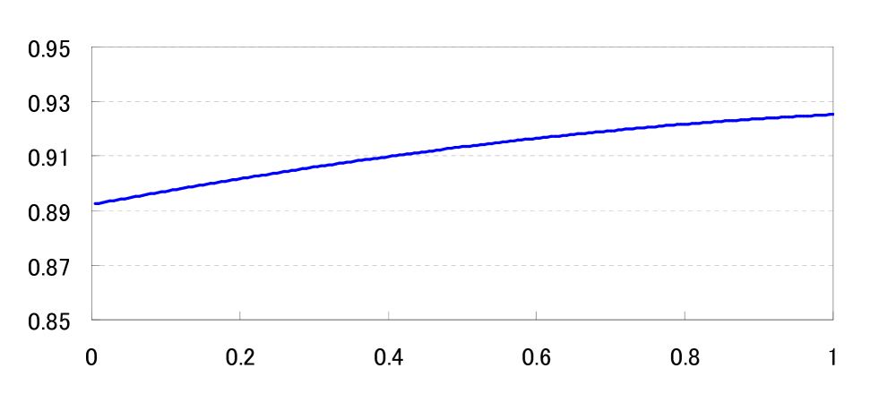
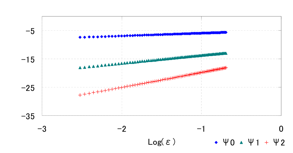
\displaystyle\displaystyle u_{\varepsilon,\pm}=\frac{\varepsilon-2\kappa\rho\pm\sqrt{4\kappa^{2}+\varepsilon^{2}-4\kappa\rho\varepsilon}}{2\varepsilon(1-\rho^{2})}.

We can easily see that $\displaystyle u_{\varepsilon,+}\nearrow\infty$ and $\displaystyle u_{\varepsilon,-}\searrow-\infty$ as $\displaystyle\varepsilon\downarrow 0$ ; thus, [A4] is satisfied. [A5] is obtained by Theorem 3.1 in Yoshikawa (2013). Finally, we numerically compute the minimum value of $\displaystyle K^{\prime\prime}_{\varepsilon}$ for each $\displaystyle\varepsilon$ to confirm [A3]. We set the parameters as $\displaystyle\kappa=1$ , $\displaystyle b=1$ , $\displaystyle x_{0}=0$ , $\displaystyle v_{0}=1$ , $\displaystyle\rho=0.3$ , $\displaystyle T=1$ , and $\displaystyle x=1$ . Then we get Figure 1, which implies that [A3] holds.

Refer to caption — Figure 1: Plots of $\displaystyle\inf_{\theta\in\mathcal{D}_{\varepsilon}}K^{\prime\prime}_{\varepsilon}(\theta)$ . The horizontal axis corresponds to $\displaystyle\varepsilon$ .

Remark 4.

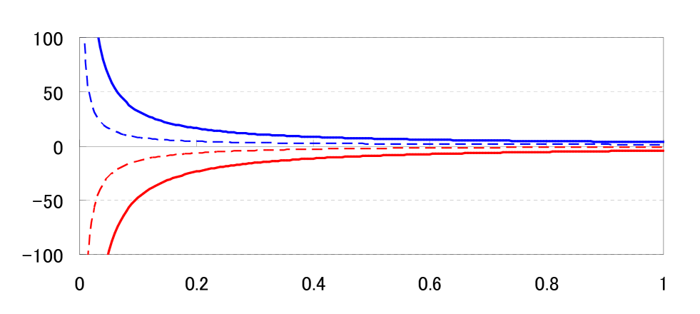
Theorem 3.1 in Rollin, Castilla, and Utzet (2010) presents a method to calculate the lower bound $\displaystyle\theta^{*}_{\varepsilon,-}$ and the upper bound $\displaystyle\theta^{*}_{\varepsilon,+}$ of the effective domain $\displaystyle\mathcal{D}_{\varepsilon}$ . When we set the parameters as above, the bounds $\displaystyle\theta^{*}_{\varepsilon,\pm}$ are obtained by

	$\displaystyle\displaystyle\theta^{*}_{\varepsilon,+}$	$\displaystyle\displaystyle=$	$\displaystyle\displaystyle\mathrm{argmin}\{\tilde{q}_{\varepsilon}(\theta)\ ;\ \theta\in(u_{\varepsilon,+},\alpha_{\varepsilon,+1})\},$
	$\displaystyle\displaystyle\theta^{*}_{\varepsilon,+}$	$\displaystyle\displaystyle=$	$\displaystyle\displaystyle\mathrm{argmax}\{\tilde{q}_{\varepsilon}(\theta)\ ;\ \theta\in(\alpha_{\varepsilon,-1},u_{\varepsilon,-})\},$

where

\displaystyle\displaystyle\tilde{q}_{\varepsilon}(\theta)=\cos\frac{\sqrt{-p_{\varepsilon}(\theta)}T}{2}+\frac{\kappa-\varepsilon\rho\theta}{\sqrt{-p_{\varepsilon}(\theta)}}\sin\frac{\sqrt{-p_{\varepsilon}(\theta)}T}{2}

and $\displaystyle\alpha_{\varepsilon,-1}<0<\alpha_{\varepsilon,+1}$ are the solutions to $\displaystyle p_{\varepsilon}(\theta)=-4\pi^{2}/T^{2}$ . Note that $\displaystyle K_{\varepsilon}(\theta)$ is given by (4.1) on $\displaystyle[u_{\varepsilon,-},u_{\varepsilon,+}]$ and by

\displaystyle\displaystyle K_{\varepsilon}(\theta)=x_{0}\theta+\frac{2\kappa b}{\varepsilon^{2}}\left\{\frac{1}{2}(\kappa-\varepsilon\rho\theta)-\log\tilde{q}_{\varepsilon}(\theta)\right\}-\frac{v_{0}(\theta-\theta^{2})\sin(\sqrt{-p_{\varepsilon}(\theta)}T/2)}{\sqrt{-p_{\varepsilon}(\theta)}\tilde{q}_{\varepsilon}(\theta)}

on $\displaystyle\mathcal{D}_{\varepsilon}\setminus[u_{\varepsilon,-},u_{\varepsilon,+}]$ . In Figure 2, we numerically calculate $\displaystyle u_{\varepsilon,\pm}$ and $\displaystyle\theta^{*}_{\varepsilon,\pm}$ for $\displaystyle\varepsilon\in(0,1]$ . This suggests the modified condition [A4’].

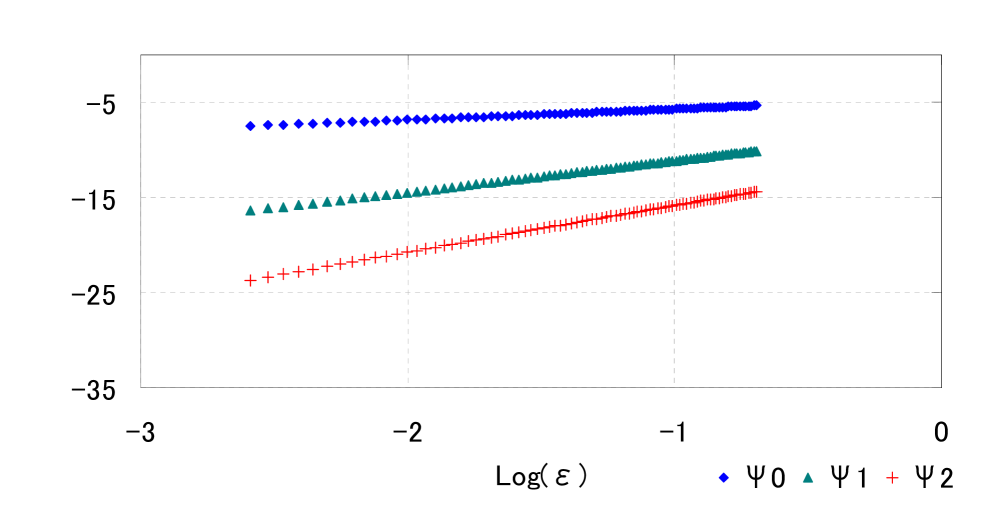
Now we verify the orders of approximate terms $\displaystyle\Psi^{\varepsilon}_{m}(\hat{w}_{\varepsilon})$ with $\displaystyle m=0,1,2$ . Figure 3 represents the log-log plot of the approximations for small $\displaystyle\varepsilon$ . In this figure, we can find the linear relationships between $\displaystyle\log|\Psi^{\varepsilon}_{m}(\hat{w}_{\varepsilon})|$ and $\displaystyle\log\varepsilon$ . We estimate their relationship by linear regression and get

$\displaystyle\displaystyle\log\|\Psi^{\varepsilon}_{0}(\hat{w}_{\varepsilon})\|$	$\displaystyle\displaystyle=$	$\displaystyle\displaystyle 1.1365\log\varepsilon-4.5611,\ \ R^{2}=0.9996,$
$\displaystyle\displaystyle\log\|\Psi^{\varepsilon}_{1}(\hat{w}_{\varepsilon})\|$	$\displaystyle\displaystyle=$	$\displaystyle\displaystyle 3.3152\log\varepsilon-7.8203,\ \ R^{2}=0.9999,$
$\displaystyle\displaystyle\log\|\Psi^{\varepsilon}_{2}(\hat{w}_{\varepsilon})\|$	$\displaystyle\displaystyle=$	$\displaystyle\displaystyle 4.9068\log\varepsilon-10.928,\ \ R^{2}=0.9999.$

Then we can numerically confirm that $\displaystyle\Psi^{\varepsilon}_{m}(\hat{w}_{\varepsilon})=O(\varepsilon^{2m+1})$ as $\displaystyle\varepsilon\rightarrow 0$ for $\displaystyle m=0,1,2$ , which is consistent with Theorem 2 and (3.4) (see also Theorem 3 in Section 6.1).

Next, we calculate the relative errors of the LR formula. We let

Normal formula	$\displaystyle\displaystyle=$	$\displaystyle\displaystyle\bar{\Phi}(\hat{w}_{\varepsilon}),$
$\displaystyle\displaystyle 0\mbox{th formula}$	$\displaystyle\displaystyle=$	$\displaystyle\displaystyle\bar{\Phi}(\hat{w}_{\varepsilon})+\Psi^{\varepsilon}_{0}(\hat{w}_{\varepsilon}),$
$\displaystyle\displaystyle 1\mbox{st formula}$	$\displaystyle\displaystyle=$	$\displaystyle\displaystyle\bar{\Phi}(\hat{w}_{\varepsilon})+\Psi^{\varepsilon}_{0}(\hat{w}_{\varepsilon})+\Psi^{\varepsilon}_{1}(\hat{w}_{\varepsilon}),$
$\displaystyle\displaystyle 2\mbox{nd formula}$	$\displaystyle\displaystyle=$	$\displaystyle\displaystyle\bar{\Phi}(\hat{w}_{\varepsilon})+\Psi^{\varepsilon}_{0}(\hat{w}_{\varepsilon})+\Psi^{\varepsilon}_{1}(\hat{w}_{\varepsilon})+\Psi^{\varepsilon}_{2}(\hat{w}_{\varepsilon}).$

We define the relative error for approximated value $\displaystyle\hat{P}$ of $\displaystyle P(X^{\varepsilon}_{T}>x)$ :

\displaystyle\displaystyle\mathrm{RE}=\left|\frac{\hat{P}}{P(X^{\varepsilon}_{T}>x)}-1\right|.

(4.2)

To find the true value of $\displaystyle P(X^{\varepsilon}_{T}>x)$ (‘True’ in Table 1), we directly calculate the integral (2.2) with $\displaystyle c=\hat{\theta}_{\varepsilon}$ .

$\displaystyle\varepsilon$	$\displaystyle P(X^{\varepsilon}_{T}>x)$					RE
$\displaystyle\varepsilon$	True	Normal	0th	1st	2nd	Normal	0th	1st	2nd
0.2	0.06622	0.06788	0.06622	0.06622	0.06622	2.51E-02	2.84E-05	3.12E-07	3.18E-09
0.4	0.06521	0.06894	0.06523	0.06521	0.06521	5.71E-02	2.88E-04	9.57E-06	4.04E-07
0.6	0.06385	0.06996	0.06392	0.06385	0.06385	9.56E-02	1.11E-03	6.76E-05	6.28E-06
0.8	0.06219	0.07093	0.06237	0.06217	0.06219	1.41E-01	2.82E-03	2.60E-04	4.11E-05
1	0.06029	0.07184	0.06063	0.06025	0.06028	1.92E-01	5.69E-03	7.22E-04	1.40E-04

Table 1: Approximated values of

\displaystyle P(X^{\varepsilon}_{T}>x)

and relative errors with

\displaystyle\varepsilon=0.2,0.4,0.6,0.8,1

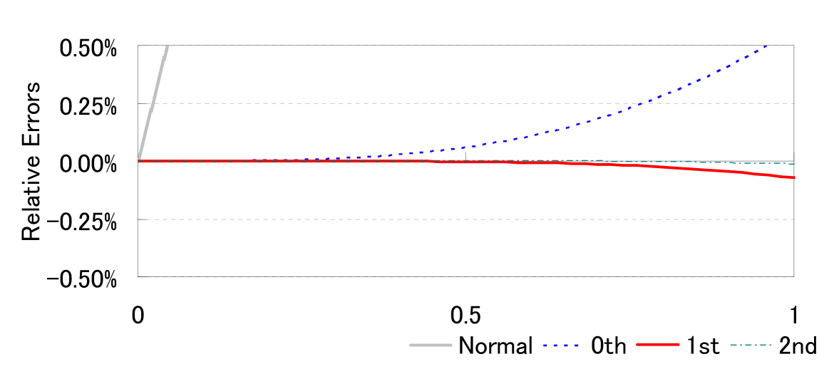
The results are shown in Table 1 and Figure 4. We see that the relative errors decrease when $\displaystyle\varepsilon$ becomes small. Moreover, we can verify that the higher order LR formula gives a more accurate approximation. In particular, the accuracies of the ‘ $\displaystyle 1$ st’ and ‘ $\displaystyle 2$ nd’ formulae are quite high, even when $\displaystyle\varepsilon$ is not small.

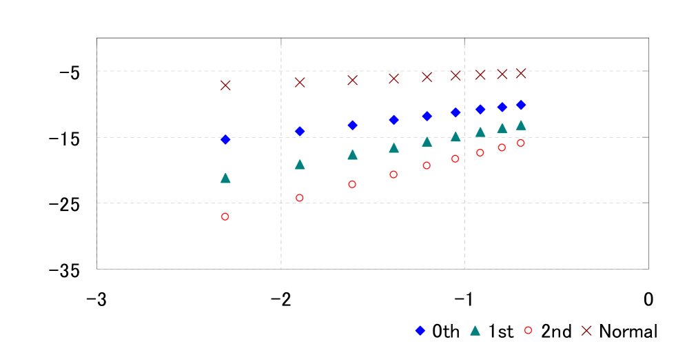
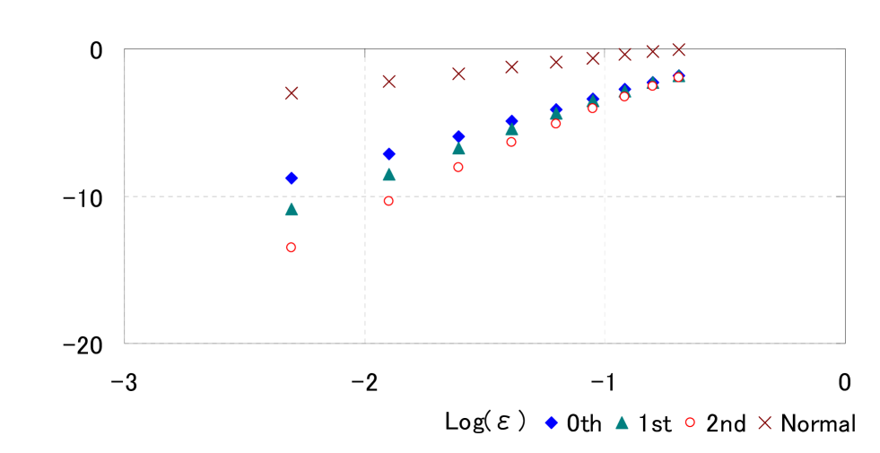
Figure 5 shows the log-log plot of the absolute errors, defined by

\displaystyle\displaystyle\mathrm{AE}=\left|\hat{P}-P(X^{\varepsilon}_{T}>x)\right|.

(4.3)

We see that there are linear relationships between $\displaystyle\log\varepsilon$ and the $\displaystyle\log\mathrm{AE}$ functions: by linear regression, we have

$\displaystyle\displaystyle\log\mathrm{AE}_{\mathrm{Normal}}$	$\displaystyle\displaystyle=$	$\displaystyle\displaystyle 1.1460\log\varepsilon-4.5447,\ \ R^{2}=0.9996,$
$\displaystyle\displaystyle\log\mathrm{AE}_{0\mathrm{th}}$	$\displaystyle\displaystyle=$	$\displaystyle\displaystyle 3.2951\log\varepsilon-7.8692,\ \ R^{2}=0.9999,$
$\displaystyle\displaystyle\log\mathrm{AE}_{1\mathrm{st}}$	$\displaystyle\displaystyle=$	$\displaystyle\displaystyle 4.9353\log\varepsilon-9.7660,\ \ R^{2}=0.9999,$
$\displaystyle\displaystyle\log\mathrm{AE}_{2\mathrm{nd}}$	$\displaystyle\displaystyle=$	$\displaystyle\displaystyle 6.9894\log\varepsilon-11.050,\ \ R^{2}=0.9999.$

These imply that the error of the $\displaystyle m$ th LR formula has order $\displaystyle O(\varepsilon^{2m+3})$ as $\displaystyle\varepsilon\rightarrow 0$ , which is consistent with (3.5) and Theorem 4 in Section 6.1.

At the end of this section, we consider the application to option pricing. We calculate the European call option price

\displaystyle\displaystyle\mathrm{Call}^{\varepsilon}=\mathrm{E}[\max\left\{\exp\left(X^{\varepsilon}_{T}\right)-L,0\right\}]

(4.4)

under the risk-neutral probability measure $\displaystyle P$ , where $\displaystyle L>0$ is the strike price.

The explicit form of $\displaystyle\mathrm{Call}^{\varepsilon}$ was obtained by Heston (1993), so we can calculate the exact value, up to the truncation error associated with numerical integration. Applying the LR formula to (4.4) was proposed by Rogers and Zane (1999). Here, we briefly review the procedure to do so. First, we rewrite (4.4) as

\displaystyle\displaystyle\mathrm{Call}^{\varepsilon}=\mathrm{E}[\exp\left(X^{\varepsilon}_{T}\right)\ ;\ X^{\varepsilon}_{T}>l]-LP(X^{\varepsilon}_{T}>l),

where $\displaystyle l=\log L$ . For the second term in the right-hand side of the above equality, we can directly apply the LR formula. To evaluate the first term, we define a new probability measure $\displaystyle Q$ (called the share measure) by the following Radon–Nikodym density

\displaystyle\displaystyle\frac{dQ}{dP}=\frac{\exp\left(X^{\varepsilon}_{T}\right)}{\mathrm{E}[\exp\left(X^{\varepsilon}_{T}\right)]}=\exp\left(-K_{\varepsilon}(1)\right)\exp\left(X^{\varepsilon}_{T}\right).

From this we obtain

\displaystyle\displaystyle\mathrm{E}[\exp\left(X^{\varepsilon}_{T}\right)\ ;\ X^{\varepsilon}_{T}>l]=\exp\left(K_{\varepsilon}(1)\right)Q(X^{\varepsilon}_{T}>l).

Now, we can easily find the CGF $\displaystyle\tilde{K}_{\varepsilon}(\theta)$ of the distribution $\displaystyle Q(X^{\varepsilon}_{T}\in\cdot)$ :

\displaystyle\displaystyle\tilde{K}_{\varepsilon}(\theta)=K_{\varepsilon}(\theta+1)-K_{\varepsilon}(1).

Obviously, $\displaystyle\tilde{K}_{\varepsilon}(\theta)$ satisfies our assumptions [A1]–[A5]. Therefore, we can apply the LR formula to $\displaystyle Q(X^{\varepsilon}_{T}>l)$ .

Now we set the initial price $\displaystyle e^{x_{0}}$ of the underlying asset as $\displaystyle 100$ and the strike price $\displaystyle L$ as 105. For the model parameters, we set $\displaystyle\kappa=6$ , $\displaystyle b=0.3^{2}$ , $\displaystyle\rho=0.3$ , and $\displaystyle v_{0}=0.2^{2}$ . We denote by $\displaystyle\mathrm{Call}^{\varepsilon}_{\mathrm{Normal}}$ , $\displaystyle\mathrm{Call}^{\varepsilon}_{0\mathrm{th}}$ , $\displaystyle\mathrm{Call}^{\varepsilon}_{1\mathrm{st}}$ and $\displaystyle\mathrm{Call}^{\varepsilon}_{2\mathrm{nd}}$ the approximations of $\displaystyle\mathrm{Call}^{\varepsilon}$ using the LR formulae ‘Normal,’ ‘ $\displaystyle 0$ th,’ ‘ $\displaystyle 1$ st’ and ‘ $\displaystyle 2$ nd’, respectively. RE and AE are the same as in (4.2) and (4.3), respectively, with tail probabilities as option prices.

$\displaystyle\varepsilon$	Call Option Price					RE
$\displaystyle\varepsilon$	True	Normal	0th	1st	2nd	Normal	0th	1st	2nd
0.2	9.352	9.367	9.352	9.352	9.352	1.62E-03	8.93E-06	5.95E-08	7.04E-10
0.4	9.358	9.419	9.357	9.358	9.358	6.46E-03	1.41E-04	3.78E-06	1.60E-07
0.6	9.337	9.471	9.330	9.337	9.337	1.43E-02	7.00E-04	4.29E-05	3.43E-06
0.8	9.291	9.523	9.271	9.293	9.291	2.50E-02	2.14E-03	2.38E-04	2.63E-05
1	9.223	9.576	9.177	9.231	9.224	3.82E-02	5.01E-03	8.79E-04	1.16E-04

Table 2: Approximated values of

\displaystyle\mathrm{Call}^{\varepsilon}

and relative errors with

\displaystyle\varepsilon=0.2,0.4,0.6,0.8,1

in the Heston SV model.

Table 2 and Figure 6 summerise the results. As in the tail probability case, we can see that the LR formulae yield highly accurate approximations.

4.2 The Wishart SV Model

Next, we introduce the Wishart SV model. The Wishart process was first studied by Bru (1991); it was first used to describe multivariate stochastic volatility by Gouriéroux (2006). Since then, modelling of multivariate stochastic volatility by using the Wishart process has been studied in several papers, such as Fonseca, Grasselli, and Tebaldi (2007, 2008), Grasselli and Tebaldi (2008), Gouriéroux, Jasiak, and Sufana (2009), and Benamid, Bensusan, and El Karoui (2010).

We consider the following SDE:

	$\displaystyle\displaystyle dY^{\varepsilon}_{t}=-\frac{1}{2}\mathrm{tr}[\Sigma^{\varepsilon}_{t}]dt+\mathrm{tr}[\sqrt{\Sigma^{\varepsilon}_{t}}(dW_{t}R^{\prime}+dB_{t}\sqrt{I-RR^{\prime}})],$
	$\displaystyle\displaystyle d\Sigma^{\varepsilon}_{t}=(\Omega^{\prime}\Omega+M\Sigma^{\varepsilon}_{t}+\Sigma^{\varepsilon}_{t}M^{\prime})dt+\varepsilon\left\{\sqrt{\Sigma^{\varepsilon}_{t}}dW_{t}Q+Q^{\prime}(dW_{t})^{\prime}\sqrt{\Sigma^{\varepsilon}_{t}}\right\},$
	$\displaystyle\displaystyle\ Y^{\varepsilon}_{0}=y_{0},\ \Sigma^{\varepsilon}_{0}=\Sigma_{0},$

where $\displaystyle I$ is the $\displaystyle n$ -dimensional unit matrix, $\displaystyle R,M,Q\in\mathbb{R}^{n}\otimes\mathbb{R}^{n}$ , and $\displaystyle\varepsilon\geq 0$ . Here, $\displaystyle\mathrm{tr}[A]$ is the trace of $\displaystyle A$ and $\displaystyle A^{\prime}$ denotes the transpose matrix of $\displaystyle A$ . $\displaystyle\Omega\in\mathbb{R}^{n}\otimes\mathbb{R}^{n}$ is assumed to satisfy

\displaystyle\displaystyle\Omega^{\prime}\Omega=\beta Q^{\prime}Q

for some $\displaystyle\beta\geq(n-1)\varepsilon^{2}$ . $\displaystyle(W_{t})_{t}$ and $\displaystyle(B_{t})_{t}$ are $\displaystyle\mathbb{R}^{n}\otimes\mathbb{R}^{n}$ -valued processes whose components are mutually independent standard Brownian motions. The process $\displaystyle(Y^{\varepsilon}_{t})_{t}$ is regarded as the log-price of a security under a risk-neutral probability measure. $\displaystyle(\Sigma^{\varepsilon}_{t})_{t}$ is an $\displaystyle n$ -dimensional matrix-valued process which describes multivariate stochastic volatility. We verify the validity of the approximation terms of the exact LR expansion for $\displaystyle\bar{F}_{\varepsilon}(x)=P(Y^{\varepsilon}_{T}>x)$ .

The explicit form of the CGF of $\displaystyle\mu_{\varepsilon}=P(Y^{\varepsilon}_{T}\in\cdot)$ is studied in Bru (1991), Fonseca, Grasselli and Tebaldi (2008), and others. To simplify, we only treat the case of $\displaystyle n=2$ and restrict the forms of $\displaystyle R,M$ and $\displaystyle Q$ as follows:

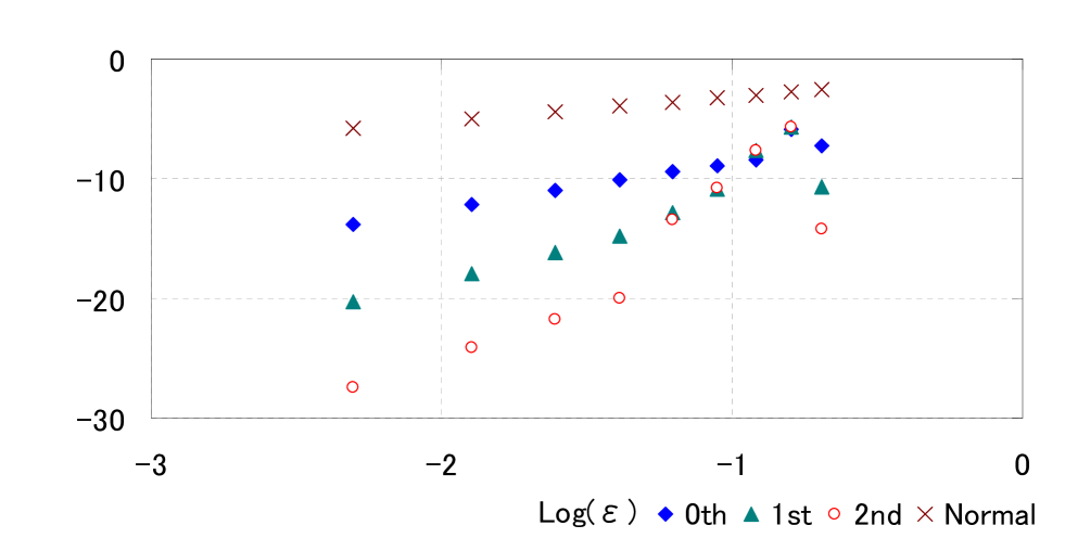
\displaystyle\displaystyle R=\left(\begin{array}[]{cc}r&0\\ 0&r\end{array}\right),\ \ M=\left(\begin{array}[]{cc}-m&0\\ 0&-m\end{array}\right),\ \ Q=\left(\begin{array}[]{cc}q&0\\ 0&q\end{array}\right),\ \ \Sigma_{0}=\left(\begin{array}[]{cc}\sigma^{2}_{0}&0\\ 0&\sigma^{2}_{0}\end{array}\right).

We set parameters as $\displaystyle r=-0.7$ , $\displaystyle q=0.25$ , $\displaystyle m=1$ , $\displaystyle\beta=3$ , $\displaystyle y_{0}=0$ , $\displaystyle\sigma_{0}=1$ , $\displaystyle T=1$ , and $\displaystyle x=1$ . Similar to the case in Section 4.1, we can find linear relationships between $\displaystyle\log|\Psi^{\varepsilon}_{m}(\hat{w}_{\varepsilon})|$ and $\displaystyle\log\varepsilon$ in Figure 7 with $\displaystyle m=0,1,2$ . Linear regression gives

$\displaystyle\displaystyle\log\|\Psi^{\varepsilon}_{0}(\hat{w}_{\varepsilon})\|$	$\displaystyle\displaystyle=$	$\displaystyle\displaystyle 0.9740\log\varepsilon-4.9496,\ \ R^{2}=0.9999,$
$\displaystyle\displaystyle\log\|\Psi^{\varepsilon}_{1}(\hat{w}_{\varepsilon})\|$	$\displaystyle\displaystyle=$	$\displaystyle\displaystyle 2.8128\log\varepsilon-10.943,\ \ R^{2}=0.9995,$
$\displaystyle\displaystyle\log\|\Psi^{\varepsilon}_{2}(\hat{w}_{\varepsilon})\|$	$\displaystyle\displaystyle=$	$\displaystyle\displaystyle 5.2875\log\varepsilon-14.474,\ \ R^{2}=0.9999.$

Thus, for this case also we can numerically confirm that $\displaystyle\Psi^{\varepsilon}_{m}(\hat{w}_{\varepsilon})=O(\varepsilon^{2m+1})$ , $\displaystyle\varepsilon\rightarrow 0$ for $\displaystyle m=0,1,2$ .

Now we investigate the relative errors of the LR formula. We compare the approximations of $\displaystyle P(Y^{\varepsilon}_{T}>x)$ by the formulae ‘Normal,’ ‘ $\displaystyle 0$ th,’ ‘ $\displaystyle 1$ st’, and ‘ $\displaystyle 2$ nd’, defined in the same way as in Section 4.1, with the true value, which is calculated by direct evaluation of the integral in (2.2).

$\displaystyle\varepsilon$	$\displaystyle P(Y^{\varepsilon}_{T}>x)$					RE
$\displaystyle\varepsilon$	True	Normal	0th	1st	2nd	Normal	0th	1st	2nd
0.2	0.06610	0.06462	0.06610	0.06610	0.06610	2.24E-02	2.97E-06	4.62E-09	1.73E-11
0.4	0.06624	0.06333	0.06623	0.06624	0.06624	4.38E-02	2.00E-05	1.88E-07	2.53E-09
0.6	0.06622	0.06198	0.06622	0.06622	0.06622	6.40E-02	5.25E-05	1.77E-06	4.76E-08
0.8	0.06604	0.06056	0.06603	0.06604	0.06604	8.30E-02	8.31E-05	7.92E-06	-6.20E-07
1	0.06568	0.05908	0.06567	0.06568	0.06568	1.00E-01	9.12E-05	4.59E-06	-2.52E-05

Table 3: Approximated values of

\displaystyle P(Y^{\varepsilon}_{T}>x)

and relative errors for

\displaystyle\varepsilon=0.2,0.4,0.6,0.8,1

Similar to the case in Section 4.1, we show the relative errors and the log-log plot of absolute errors of the formulae in Table 3 and Figure 8. We can also confirm that the LR formulae are highly accurate. Using the data shown in Figure 8, we get the linear regression results

$\displaystyle\displaystyle\log\mathrm{AE}_{\mathrm{Normal}}$	$\displaystyle\displaystyle=$	$\displaystyle\displaystyle 0.9732\log\varepsilon-4.9507,\ \ R^{2}=0.9999,$
$\displaystyle\displaystyle\log\mathrm{AE}_{0\mathrm{th}}$	$\displaystyle\displaystyle=$	$\displaystyle\displaystyle 2.7930\log\varepsilon-10.979,\ \ R^{2}=0.9994,$
$\displaystyle\displaystyle\log\mathrm{AE}_{1\mathrm{st}}$	$\displaystyle\displaystyle=$	$\displaystyle\displaystyle 5.3063\log\varepsilon-13.339,\ \ R^{2}=0.9999,$
$\displaystyle\displaystyle\log\mathrm{AE}_{2\mathrm{nd}}$	$\displaystyle\displaystyle=$	$\displaystyle\displaystyle 7.1747\log\varepsilon-15.937,\ \ R^{2}=0.9999,$

which suggest (3.5).

At the end of this section, we confirm the validity for application in option pricing. Similarly to (4.4), we consider the European call option

\displaystyle\displaystyle\mathrm{Call}^{\varepsilon}=\mathrm{E}[\max\left\{\exp\left(Y^{\varepsilon}_{T}\right)-L,0\right\}]

with the strike price $\displaystyle L>0$ . To find the true value of the option price, we apply a closed-form formula proposed in Benabid, Bensusan, and El Karoui (2010). We set the initial price of the underlying asset as $\displaystyle e^{y0}=100$ and $\displaystyle L=105$ . For the initial volatility, we put $\displaystyle\sigma_{0}=0.25$ . Other parameters are the same as in the previous case.

$\displaystyle\varepsilon$	Call Option Price					RE
$\displaystyle\varepsilon$	True	Normal	0th	1st	2nd	Normal	0th	1st	2nd
0.2	10.90	10.91	10.90	10.90	10.90	1.13E-03	1.50E-06	8.61E-09	3.15E-11
0.4	10.76	10.80	10.76	10.76	10.76	4.58E-03	2.10E-05	4.56E-05	4.62E-05
0.6	10.60	10.70	10.59	10.59	10.59	9.88E-03	4.37E-04	3.08E-04	3.02E-04
0.8	10.46	10.60	10.40	10.41	10.41	1.27E-02	5.71E-03	5.29E-03	5.25E-03
1	10.15	10.49	10.20	10.21	10.21	3.37E-02	4.33E-03	5.41E-03	5.55E-03

Table 4: Approximations of

\displaystyle\mathrm{Call}^{\varepsilon}

and relative errors with

\displaystyle\varepsilon=0.2,0.4,0.6,0.8,1

in the Wishart SV model.

The results are shown in Table 4 and Figure 9. Although the linear relationships are not as clear as in Figure 6, we can see that the LR formulae are highly accurate in each case.

5 Proofs

5.1 Proof of Theorem 1

In this subsection, we justify the formal calculations shown in Section 2. For ease of readability, we omit $\displaystyle\varepsilon$ from the notation used in this section.

Proposition 1.

Assume $\displaystyle\mathrm{[A1]}$ – $\displaystyle\mathrm{[A2]}$ hold. Then

\displaystyle\displaystyle\bar{F}(x)\ =\ \frac{1}{2\pi i}\int^{c+i\infty}_{c-i\infty}\exp(K(\theta)-x\theta)\frac{d\theta}{\theta}

for $\displaystyle c\in\mathcal{O}\setminus\{0\}$ .

Proof.

Without loss of generality, we may assume $\displaystyle c>0$ and $\displaystyle x\geq 0$ . By [A2] and Theorem 3.3.5 in Durrett (2010), the density function $\displaystyle f$ of $\displaystyle\mu$ exists and is bounded and continuous. Moreover,

\displaystyle\displaystyle f(y)=\frac{1}{2\pi}\int_{\mathbb{R}}e^{-i\xi y}\varphi(\xi)d\xi

holds, where $\displaystyle\varphi(\xi)=\exp(K(i\xi))$ is the characteristic function of $\displaystyle\mu$ . Then we have for each $\displaystyle R>x$ that

\displaystyle\displaystyle\mu((x,R])=\frac{1}{2\pi}\int^{R}_{x}\int_{\mathbb{R}}e^{-i\xi y}\varphi(\xi)d\xi dy=\frac{1}{2\pi i}\int^{i\infty}_{-i\infty}F(z)dz

by Fubini’s theorem, where

\displaystyle\displaystyle F(z)=\int_{\mathbb{R}}\int^{R}_{x}e^{(s-y)z}f(s)dyds.

Now, consider the four lines $\displaystyle\Gamma_{1},\ldots,\Gamma_{4}\subset\mathbb{C}$ , defined as

	$\displaystyle\displaystyle\Gamma_{1}=\{it\ ;\ t\in[-l,l]\},\ \ \Gamma_{2}=\{t+il\ ;\ t\in[0,c]\},$
	$\displaystyle\displaystyle\Gamma_{3}=\{t-il\ ;\ t\in[0,c]\},\ \ \Gamma_{4}=\{c+it\ ;\ t\in[-l,l]\}$

for a given $\displaystyle l>0$ . By Cauchy’s integral theorem, we have

\displaystyle\displaystyle\int_{\Gamma_{1}\cup\Gamma_{2}\cup\Gamma_{3}\cup\Gamma_{4}}F(z)dz=0.

(5.1)

Here, we observe that

$\displaystyle\displaystyle\int_{\Gamma_{2}\cup\Gamma_{3}}F(z)dz$	$\displaystyle\displaystyle=$	$\displaystyle\displaystyle 2i\int^{c}_{0}\int_{\mathbb{R}}\int^{R}_{x}e^{(s-y)t}f(s)\sin l(s-y)dydsdt$
	$\displaystyle\displaystyle=$	$\displaystyle\displaystyle 2i\int^{c}_{0}\int_{\mathbb{R}}\frac{f(s)}{t^{2}+l^{2}}\Big{[}e^{(s-x)t}(-l\cos l(s-x)+t\sin l(s-x))$
		$\displaystyle\displaystyle\hskip 85.35826pt+e^{(s-R)t}(l\cos l(s-R)-t\sin l(s-R))\Big{]}dsdt$

to conclude

\displaystyle\displaystyle\left|\int_{\Gamma_{2}\cup\Gamma_{3}}F(z)dz\right|\ \leq\ \frac{4(l+c)c}{l^{2}}\int_{\mathbb{R}}e^{cs}f(s)ds=\frac{4(l+c)c}{l^{2}}e^{K(c)}.

Since $\displaystyle c\in\mathcal{O}$ , the integral on the right-hand side is finite. Thus, the left-hand side must converge to zero as $\displaystyle l\rightarrow\infty$ . Combining this result with (5.1), we obtain that

	$\displaystyle\displaystyle\mu((x,R])\ =\ \frac{1}{2\pi i}\lim_{l\rightarrow\infty}\int_{\Gamma_{1}}F(z)dz\ =\ \frac{1}{2\pi i}\lim_{l\rightarrow\infty}\int_{\Gamma_{4}}F(z)dz$
	$\displaystyle\displaystyle=\frac{1}{2\pi i}\int^{c+i\infty}_{c-i\infty}\int_{\mathbb{R}}\int^{R}_{x}e^{(s-y)z}f(s)dydsdz\ =\ \frac{1}{2\pi i}\int^{c+i\infty}_{c-i\infty}\int^{R}_{x}e^{K(z)-yz}dydz.\ \ \ \ \$		(5.2)

Since

\displaystyle\displaystyle\int^{c+i\infty}_{c-i\infty}\int^{\infty}_{0}|e^{K(z)-yz}|dy|dz|\leq\frac{1}{c}e^{K(c)}<\infty,

we can take the limit $\displaystyle R\rightarrow\infty$ on the right-hand side of (5.2); we conclude that

\displaystyle\displaystyle\bar{F}(x)=\frac{1}{2\pi i}\int^{c+i\infty}_{c-i\infty}\int^{\infty}_{x}e^{K(z)-yz}dydz=\frac{1}{2\pi i}\int^{c+i\infty}_{c-i\infty}e^{K(z)-xz}\frac{dz}{z},

which is the assertion of Proposition 1. ∎

Now, we present the rigorous definition of the change of variables (2.5). For each $\displaystyle\theta\in\mathcal{D}$ , we can define $\displaystyle w=w(\theta)\in\mathbb{R}$ by

\displaystyle\displaystyle w(\theta)=\hat{w}+\mathrm{sgn}(\theta-\hat{\theta})\sqrt{2\left\{\left(K(\theta)-x\theta\right)-\left(K(\hat{\theta})-x\hat{\theta}\right)\right\}}.

(5.3)

Obviously, $\displaystyle w(\theta)$ is analytic on $\displaystyle\mathcal{O}\setminus\{\hat{\theta}\}$ . Moreover, by straightforward calculation we observe

\displaystyle\displaystyle\frac{dw}{d\theta}=\mathrm{sgn}(\theta-\hat{\theta})\cdot\frac{K^{\prime}(\theta)-x}{\sqrt{\hat{w}^{2}+2(K(\theta)-x\theta)}}=\frac{K^{\prime}(\theta)-x}{w(\theta)-\hat{w}}.

(5.4)

Here we see that $\displaystyle w(\theta)$ is also analytic at $\displaystyle\hat{\theta}$ . Indeed, similar to (2.4), we have

\displaystyle\displaystyle w(\theta)=\hat{w}+\mathrm{sgn}(\theta-\hat{\theta})\sqrt{k(\theta)}|\theta-\hat{\theta}|=\hat{w}+\sqrt{k(\theta)}(\theta-\hat{\theta}),

where

\displaystyle\displaystyle k(\theta)=\int^{1}_{0}K^{\prime\prime}(\hat{\theta}+u(\theta-\hat{\theta}))du.

By [A2], $\displaystyle k(\theta)$ is positive, and thus $\displaystyle\sqrt{k(\theta)}$ is real analytic. As a consequence, the function $\displaystyle w(\theta)$ is real analytic on $\displaystyle\mathcal{O}$ . Now we can take the limit $\displaystyle\theta\rightarrow\hat{\theta}$ in (5.5) to obtain

\displaystyle\displaystyle w^{\prime}(\hat{\theta})=\lim_{\theta\rightarrow\hat{\theta}}\frac{K^{\prime}(\theta)-x}{w-\hat{w}}=\lim_{\theta\rightarrow\hat{\theta}}\frac{K^{\prime\prime}(\theta)}{w^{\prime}(\theta)}

by using l’Hôpital’s rule. This implies that $\displaystyle(w^{\prime}(\hat{\theta}))^{2}=K^{\prime\prime}(\hat{\theta})\neq 0$ . Therefore, we deduce that there exist a neighbourhood $\displaystyle U\subset\mathbb{C}$ of $\displaystyle w(\hat{\theta})=\hat{w}$ and a holomorphic function $\displaystyle\theta(w)$ on $\displaystyle U$ such that $\displaystyle\theta(w(z))=z$ for $\displaystyle z\in U$ .

Here we remark that

Lemma 1.

$\displaystyle\theta\notin\mathcal{D}$ implies $\displaystyle K^{\prime}(\theta)$ does not lie on $\displaystyle\mathbb{R}$ .

Proof.

Let $\displaystyle y\in\mathbb{R}$ . By [A2], we have $\displaystyle K^{\prime\prime}(y)\neq 0$ . Thus, we can find a neighbourhood $\displaystyle U$ of $\displaystyle K^{\prime}(y)$ and an analytic inverse function function $\displaystyle(K^{\prime})^{-1}$ of $\displaystyle K^{\prime}$ defined on $\displaystyle U$ . On the other hand, [A2] implies that $\displaystyle(K^{\prime})^{-1}|_{U\cap\mathbb{R}}$ is an analytic $\displaystyle\mathcal{D}$ -valued function, hence $\displaystyle(K^{\prime})^{-1}(y)\in\mathcal{D}$ . ∎

Lemma 1 immediately implies

Corollary 1.

Let $\displaystyle z\in\mathcal{D}\times i\mathbb{R}$ . If $\displaystyle z\neq\hat{\theta}$ , then $\displaystyle K^{\prime}(z)\neq x$ ; hence, $\displaystyle w^{\prime}(\theta)\neq 0$ .

Now, we consider an analytic continuation of $\displaystyle\theta(w)$ . Until the end of this section, we will assume [A1]–[A2] and [B1]–[B3] hold. By [B2], (5.4) and Corollary 1, we can define the analytic function $\displaystyle\theta(w)$ on an open set $\displaystyle\hat{U}$ which contains a convex set that includes the line $\displaystyle\{\hat{w}\}\times i\mathbb{R}$ and the curve $\displaystyle\{w(\hat{\theta}+it)\ ;\ t\in\mathbb{R}\}$ . Note that (5.4) immediately implies

\displaystyle\displaystyle\theta^{\prime}(w)=\frac{w-\hat{w}}{K^{\prime}(\theta(w))-x}

(5.5)

for each $\displaystyle w\neq\hat{w}$ .

By definition, the relation (2.5) holds everywhere on $\displaystyle\hat{U}$ . Therefore, if we define the curves $\displaystyle\eta$ and $\displaystyle\gamma$ as

\displaystyle\displaystyle\eta=\{\hat{\theta}+it\ ;\ t\in\mathbb{R}\},\ \ \gamma=\{w(\theta)\ ;\ \theta\in\eta\},

then $\displaystyle\theta(w)$ can be also defined and is analytic on $\displaystyle\gamma$ . Then, we can apply the change of variables to obtain

\displaystyle\displaystyle\bar{F}(x)\ =\ \frac{1}{2\pi i}\int_{\eta}\exp(K(\theta)-x\theta)\frac{d\theta}{\theta}\ =\ \int_{\gamma}\exp\left(\frac{1}{2}w^{2}-\hat{w}w\right)\frac{\theta^{\prime}(w)}{\theta(w)}dw.

In Section 2, we need the condition $\displaystyle\hat{\theta}\neq 0$ . In this section we only consider the case where $\displaystyle\hat{\theta}>0$ ; the arguments are analogous for the case where $\displaystyle\hat{\theta}<0$ . In any case, we have $\displaystyle\hat{\theta}\neq 0$ and thus $\displaystyle\eta$ does not pass $\displaystyle 0$ . Here, we see that $\displaystyle\hat{w}>0$ . Indeed, if $\displaystyle\hat{w}=0$ , then the inequality in (2.4) must be changed to equality. However, the assumptions $\displaystyle\hat{\theta}>0$ and [A2] imply that the left-hand side of (2.4) is positive. This is a contradiction. Moreover, by its definition, $\displaystyle\hat{w}$ must be nonnegative. These arguments imply that $\displaystyle\gamma$ does not exceed $\displaystyle 0$ .

Proposition 2.

\displaystyle\displaystyle\int_{\gamma}\exp\left(\frac{1}{2}w^{2}-\hat{w}w\right)\frac{\theta^{\prime}(w)}{\theta(w)}dw

\displaystyle\displaystyle=

\displaystyle\displaystyle\int^{\hat{w}+i\infty}_{\hat{w}-i\infty}\exp\left(\frac{1}{2}w^{2}-\hat{w}w\right)\frac{\theta^{\prime}(w)}{\theta(w)}dw.

To prove this proposition, we prepare a lemma.

Lemma 2.

$\displaystyle|\theta(w)-\hat{\theta}|\geq|w-\hat{w}|/\sqrt{C}$ .

Proof.

By [B1] and Taylor’s theorem, we have

\displaystyle\displaystyle|w-\hat{w}|^{2}=2|K(\theta(w))-x\theta(w)-(K(\hat{\theta})-x\hat{\theta})|\leq C|\theta(w)-\hat{\theta}|^{2},

which implies the asserted statement. ∎

Proof of Proposition 2.

By Cauchy’s integral theorem, it suffices to show that

\displaystyle\displaystyle\lim_{l\rightarrow\pm\infty}\sup_{c\in\mathcal{O}\cap M}\left|\int_{L^{c}_{l}}\exp\left(\frac{1}{2}w^{2}-\hat{w}w\right)\frac{\theta^{\prime}(w)}{\theta(w)}dw\right|=0

(5.6)

for each compact set $\displaystyle M$ in $\displaystyle(0,\infty)$ , where $\displaystyle L^{c}_{l}=\{\hat{w}+t(c-\hat{w})+il\ ;\ t\in[0,1]\}$ and $\displaystyle l\in\mathbb{R}$ . By (5.5), we get

	$\displaystyle\displaystyle\left\|\int_{L^{c}_{l}}\exp\left(\frac{1}{2}w^{2}-\hat{w}w\right)\frac{\theta^{\prime}(w)}{\theta(w)}dw\right\|$	(5.7)
$\displaystyle\displaystyle\leq$	$\displaystyle\displaystyle\|c-\hat{w}\|\exp\left(-\frac{\hat{w}^{2}+l^{2}}{2}\right)\int^{1}_{0}\exp\left(\frac{1}{2}t^{2}(c-\hat{w})^{2}\right)\left\|\frac{t(c-\hat{w})+il}{(K^{\prime}(\theta)-x)\theta}\right\|dt$
$\displaystyle\displaystyle\leq$	$\displaystyle\displaystyle\exp\left(\frac{c^{2}-l^{2}}{2}\right)\frac{(\|c\|+\|\hat{w}\|)(\|c\|+\|\hat{w}\|+\|l\|)}{\inf_{w\in L^{c}_{l}}\|(K^{\prime}(\theta(w))-x)\theta(w)\|}.$

By [B1] and Lemma 2, we observe

\displaystyle\displaystyle\inf_{w\in L^{c}_{l}}|(K^{\prime}(\theta(w))-x)\theta(w)|\geq\delta\inf_{w\in L^{c}_{l}}|\theta(w)-\hat{\theta}|\inf_{w\in L^{c}_{l}}|\theta|\geq\delta\cdot\frac{|l|}{\sqrt{C}}\cdot\left(\frac{|l|}{\sqrt{C}}-|\hat{\theta}|\right)

for sufficiently large magnitudes of $\displaystyle l$ . Hence, we obtain (5.6) from (5.7). ∎

Proof of Theorem 1.

From Propositions 1 and 2, we get (2.6). Now we verify the holomorphicity of $\displaystyle\psi$ on $\displaystyle\{\hat{w}\}\times i\mathbb{R}$ . We define

\displaystyle\displaystyle h(w)=\log\theta(w)-\log w=\log g(w),\ \ g(w)=\frac{\theta(w)}{w}

(5.8)

when $\displaystyle\theta(w)$ is defined and let $\displaystyle w\neq 0$ , where $\displaystyle\log z$ is the principal value of the logarithm of $\displaystyle z$ . Since $\displaystyle\theta(w)$ is analytic on the line $\displaystyle\{\hat{w}\}\times i\mathbb{R}$ , $\displaystyle h$ is also analytic. We can easily see that $\displaystyle h^{\prime}(w)=\psi(w)$ . This implies that $\displaystyle\psi(w)$ is also analytic; this permits the following Taylor series expansion:

\displaystyle\displaystyle\psi(w)=\sum^{\infty}_{n=0}\frac{\psi^{(n)}(\hat{w})}{n!}(w-\hat{w})^{n}

(5.9)

for $\displaystyle w\in\{\hat{w}\}\times i\mathbb{R}$ .

To complete the proof of Theorem 1, it suffices to check the calculations in (2.7). Using (5.9) and the relation

\displaystyle\displaystyle\int^{\infty}_{-\infty}e^{-y^{2}/2}y^{n}dy=\sqrt{2\pi}(n-1)!!\ (\mbox{$\displaystyle n$ is even}),\ 0\ (\mbox{$\displaystyle n$ is odd}),

(5.10)

we have

			$\displaystyle\displaystyle\sum^{\infty}_{n=0}\frac{1}{n!}\int^{\infty}_{-\infty}e^{-y^{2}/2}\|\psi^{(n)}(\hat{w})\|\cdot\|y\|^{n}dy$
		$\displaystyle\displaystyle\leq$	$\displaystyle\displaystyle\sqrt{2\pi}\|\psi(\hat{w})\|+\sum^{\infty}_{m=1}\frac{1}{(2m)!}\{\|\psi^{(2m)}(\hat{w})\|+\|\psi^{(2m-1)}(\hat{w})\|\}\int^{\infty}_{-\infty}e^{-y^{2}/2}(y^{2m}+1)dy$
		$\displaystyle\displaystyle\leq$	$\displaystyle\displaystyle\sqrt{2\pi}\left\{\|\psi(\hat{w})\|+2\sum^{\infty}_{m=1}\frac{\|\psi^{(2m)}(\hat{w})\|+\|\psi^{(2m-1)}(\hat{w})\|}{(2m)!!}\right\}.$

By [B3], the right-hand side of the above inequality is finite. Thus, we can apply Fubini’s theorem and we can interchange the sum and the integral in (2.7). That is,

\displaystyle\displaystyle\int^{\infty}_{-\infty}e^{-y^{2}/2}\sum^{\infty}_{n=0}\frac{\psi^{(n)}(\hat{w})}{n!}(iy)^{n}dy=\sum^{\infty}_{n=0}\frac{\psi^{(n)}(\hat{w})}{n!}i^{n}\int^{\infty}_{-\infty}e^{-y^{2}/2}y^{n}dy.

We finish the proof of Theorem 1 by using (5.10) again. ∎

5.2 Proof of Theorem 2

For simplicity, we only consider the case $\displaystyle\hat{\theta}_{0}>0$ . First, we introduce the following lemma.

Lemma 3.

$\displaystyle\hat{\theta}_{\varepsilon}\longrightarrow\hat{\theta}_{0}$ , $\displaystyle\hat{w}_{\varepsilon}\longrightarrow\hat{w}_{0}$ as $\displaystyle\varepsilon\rightarrow 0$ .

Proof.

First, we check that $\displaystyle(\hat{\theta}_{\varepsilon})_{\varepsilon}$ is bounded. By (2.1), we have

\displaystyle\displaystyle\hat{\theta}_{\varepsilon}=(K^{\prime}_{\varepsilon})^{-1}(x)-(K^{\prime}_{\varepsilon})^{-1}(m_{\varepsilon})=\int^{1}_{0}\frac{du}{K^{\prime\prime}_{\varepsilon}((K^{\prime}_{\varepsilon})^{-1}(m_{\varepsilon}+u(x-m_{\varepsilon})))}(x-m_{\varepsilon}),

where $\displaystyle m_{\varepsilon}=K^{\prime}_{\varepsilon}(0)$ . By [A5], we see that $\displaystyle(m_{\varepsilon})_{\varepsilon}$ is bounded. Thus, from [A3], we get

\displaystyle\displaystyle|\hat{\theta}_{\varepsilon}|\leq\frac{1}{\delta_{0}}(|x|+\max_{\varepsilon}|m_{\varepsilon}|)<\infty.

Second, we observe that

\displaystyle\displaystyle x-K^{\prime}_{\varepsilon}(\hat{\theta}_{0})=K^{\prime\prime}_{\varepsilon}(\hat{\theta}_{0})(\hat{\theta}_{\varepsilon}-\hat{\theta}_{0})+\frac{1}{2}\int^{1}_{0}(1-u)^{2}K^{\prime\prime\prime}_{\varepsilon}(\hat{\theta}_{0}+u(\hat{\theta}_{\varepsilon}-\hat{\theta}_{0}))du(\hat{\theta}_{\varepsilon}-\hat{\theta}_{0})^{2}

to arrive at

\displaystyle\displaystyle|\hat{\theta}_{\varepsilon}-\hat{\theta}_{0}|\leq\frac{1}{\delta_{0}}\left\{|x-K^{\prime}_{\varepsilon}(\hat{\theta}_{0})|+\frac{1}{2}\sup_{y\in C}|K^{\prime\prime\prime}_{\varepsilon}(y)|\cdot\sup_{\varepsilon}|\hat{\theta}_{\varepsilon}-\hat{\theta}_{0}|^{2}\right\}

for some compact set $\displaystyle C\subset\mathbb{R}$ . Letting $\displaystyle\varepsilon\rightarrow 0$ , we get the former assertion. The latter assertion follows immediately. ∎

The above lemma implies the following corollary.

Corollary 2.

There is a $\displaystyle\delta_{1}>0$ such that $\displaystyle\hat{\theta}_{\varepsilon},\ \hat{w}_{\varepsilon}>0$ for $\displaystyle\varepsilon\in[0,\delta_{1})$ .

Proof.

Since $\displaystyle\hat{\theta}_{\varepsilon}\longrightarrow\hat{\theta}_{0}>0$ , we can find some $\displaystyle\delta_{1}>0$ such that $\displaystyle\hat{\theta}_{\varepsilon}>\hat{\theta}_{0}/2>0$ holds for $\displaystyle\varepsilon<\delta_{1}$ . The relation $\displaystyle\hat{w}_{\varepsilon}>0$ is obtained in the same way by using $\displaystyle\hat{w}_{0}=\sqrt{K^{\prime\prime}_{0}(0)}\hat{\theta}_{0}>0$ . ∎

By the above corollary, we may assume that $\displaystyle\hat{\theta}_{\varepsilon}$ and $\displaystyle\hat{w}_{\varepsilon}$ are strictly positive.

Proposition 3.

$\displaystyle\hat{w}_{\varepsilon}-\sqrt{K^{\prime\prime}_{\varepsilon}(\hat{\theta}_{\varepsilon})}\hat{\theta}_{\varepsilon}=O(\varepsilon)$ as $\displaystyle\varepsilon\rightarrow 0$ .

Proof.

Since $\displaystyle(\hat{\theta}_{\varepsilon})_{\varepsilon}$ and $\displaystyle(\hat{w}_{\varepsilon})_{\varepsilon}$ are bounded and away from zero, it suffices to show that $\displaystyle\hat{w}^{2}_{\varepsilon}-K^{\prime\prime}_{\varepsilon}(\hat{\theta}_{\varepsilon})\hat{\theta}^{2}_{\varepsilon}=O(\varepsilon)$ as $\displaystyle\varepsilon\rightarrow 0$ . From the definition of $\displaystyle\hat{w}_{\varepsilon}$ , we have

\displaystyle\displaystyle\hat{w}_{\varepsilon}^{2}=2(-K_{\varepsilon}(\hat{\theta}_{\varepsilon})+K^{\prime}_{\varepsilon}(\hat{\theta}_{\varepsilon})\hat{\theta}_{\varepsilon}).

Using $\displaystyle K_{\varepsilon}(0)=0$ and Taylor’s theorem, we get

\displaystyle\displaystyle\hat{w}^{2}_{\varepsilon}-K^{\prime\prime}_{\varepsilon}(\hat{\theta}_{\varepsilon})\hat{\theta}^{2}_{\varepsilon}=\hat{\theta}_{\varepsilon}^{2}\int^{1}_{0}K^{\prime\prime\prime}_{\varepsilon}(-u\hat{\theta}_{\varepsilon})(1-u)^{2}du.

Therefore,

\displaystyle\displaystyle|\hat{w}^{2}_{\varepsilon}-K^{\prime\prime}_{\varepsilon}(\hat{\theta}_{\varepsilon})\hat{\theta}^{2}_{\varepsilon}|\leq\sup_{|y|\leq\hat{\theta}_{\varepsilon}}y^{2}|K^{\prime\prime\prime}_{\varepsilon}(y)|=O(\varepsilon)\ \ \mbox{as}\ \ \varepsilon\rightarrow 0,

from which our assertion follows. ∎

We write

\displaystyle\displaystyle\hat{\theta}^{\prime}_{\varepsilon}=\frac{d\theta}{dw}(\hat{w}_{\varepsilon})=\lim_{w\rightarrow\hat{w}_{\varepsilon}}\frac{d\theta}{dw}(\hat{w}_{\varepsilon}).

Note that $\displaystyle\hat{\theta}^{\prime}_{\varepsilon}$ exists, because $\displaystyle\theta(w)$ is analytic at $\displaystyle\hat{w}_{\varepsilon}$ . Similarly, we can define

\displaystyle\displaystyle\hat{\theta}^{(n)}_{\varepsilon}=\frac{d^{n}\theta}{dw^{n}}(\hat{w}_{\varepsilon})=\lim_{w\rightarrow\hat{w}_{\varepsilon}}\frac{d^{n}\theta}{dw^{n}}(\hat{w}_{\varepsilon})

for each $\displaystyle n$ . The next proposition is frequently used in the calculations shown later.

Proposition 4.

$\displaystyle\hat{\theta}^{\prime}_{\varepsilon}=1/\sqrt{K^{\prime\prime}(\hat{\theta}_{\varepsilon})}$ .

Proof.

Since both the numerator and the denominator in the right-hand side of (5.5) converge to zero with $\displaystyle w\rightarrow\hat{w}_{\varepsilon}$ , we can apply l’Hôpital’s rule to obtain

\displaystyle\displaystyle\hat{\theta}^{\prime}_{\varepsilon}=\lim_{w\rightarrow\hat{w}_{\varepsilon}}\frac{w-\hat{w}_{\varepsilon}}{K^{\prime}(\theta(w))-x}=\lim_{w\rightarrow\hat{w}_{\varepsilon}}\frac{1}{K^{\prime\prime}(\theta(w))\theta^{\prime}(w)}=\frac{1}{K^{\prime\prime}(\hat{\theta}_{\varepsilon})\hat{\theta}^{\prime}_{\varepsilon}}.

Solving this equation for $\displaystyle\hat{\theta}^{\prime}_{\varepsilon}$ , we obtain the desired assertion. ∎

Recall that the function $\displaystyle g(w)$ defined in (5.8) is analytic on $\displaystyle\hat{\mathcal{O}}_{\varepsilon,+}:=\{w(\theta)\ ;\ \theta\in\mathcal{O}_{\varepsilon}\cap(0,\infty)\}$ . The following lemma is straightforward by using mathematical induction.

Lemma 4.

For each $\displaystyle n=0,1,2,\ldots$ and $\displaystyle w\in\hat{\mathcal{O}}_{\varepsilon,+}$ ,

\displaystyle\displaystyle g^{(n)}(w)=\frac{\theta^{(n)}(w)-ng^{(n-1)}(w)}{w}.

Note that $\displaystyle g(\hat{w}_{\varepsilon})=\hat{\theta}_{\varepsilon}/\hat{w}_{\varepsilon}>0$ . Therefore, we can define $\displaystyle h(w)=\log g(w)$ on a neighbourhood of $\displaystyle\hat{w}_{\varepsilon}$ . Obviously, we have $\displaystyle\psi(w)=h^{\prime}(w)$ . Hence,

\displaystyle\displaystyle\psi^{(2m)}(\hat{w}_{\varepsilon})=h^{(2m+1)}(\hat{w}_{\varepsilon}).

(5.11)

Different but nevertheless straightforward calculations give

$\displaystyle\displaystyle h^{\prime}(w)$	$\displaystyle\displaystyle=$	$\displaystyle\displaystyle\frac{g^{\prime}(w)}{g(w)},$
$\displaystyle\displaystyle h^{\prime\prime}(w)$	$\displaystyle\displaystyle=$	$\displaystyle\displaystyle\frac{g^{\prime\prime}(w)}{g(w)}-\frac{(g^{\prime}(w))^{2}}{g(w)^{2}},$	(5.12)
$\displaystyle\displaystyle h^{\prime\prime\prime}(w)$	$\displaystyle\displaystyle=$	$\displaystyle\displaystyle\frac{g^{\prime\prime\prime}(w)}{g(w)}-\frac{3g^{\prime}(w)g^{\prime\prime}(w)}{g(w)^{2}}+\frac{2(g^{\prime}(w))^{3}}{g(w)^{3}}.$

We can show by induction the following.

Lemma 5.

For each $\displaystyle n$ and $\displaystyle w\in\hat{\mathcal{O}}_{\varepsilon,+}$ ,

\displaystyle\displaystyle h^{(n)}(w)=\sum^{m_{n}}_{k=1}\left(\frac{a_{k}}{g(w)^{b_{k}}}\prod^{n}_{i=0}(g^{(c_{i,k})}(w))^{d_{i,k}}\right)

for some $\displaystyle m_{n},a_{k},b_{k},c_{i,k}$ and $\displaystyle d_{i,k}$ with $\displaystyle\sum^{n}_{i=0}c_{i_{k}}d_{i_{k}}=n$ .

By (5.11), Lemmas 3 and 5, it suffices to consider the estimation of the order of $\displaystyle g^{(m)}(\hat{w}_{\varepsilon})$ for $\displaystyle m\in\mathbb{N}$ . The next proposition gives the order estimate of $\displaystyle g^{\prime}(\hat{w}_{\varepsilon})$ .

Proposition 5.

$\displaystyle g^{\prime}(\hat{w}_{\varepsilon})=O(\varepsilon)$ as $\displaystyle\varepsilon\rightarrow 0$ .

Proof.

By Lemma 4, we have

\displaystyle\displaystyle wg^{\prime}(w)=\theta^{\prime}(w)-g(w)=\frac{w\theta^{\prime}(w)-\theta(w)}{w}.

Combining this with (5.5), we get

\displaystyle\displaystyle wg^{\prime}(w)=\frac{w(w-\hat{w}_{\varepsilon})-\theta(w)(K^{\prime}(\theta(w))-x)}{w(K^{\prime}(\theta(w))-x)}.

(5.13)

Letting $\displaystyle w\rightarrow\hat{w}_{\varepsilon}$ , both the numerator and the denominator of the right-hand side of (5.13) converge to zero. Then, we can apply l’Hôpital’s rule to obtain

	$\displaystyle\displaystyle\lim_{w\rightarrow\hat{w}_{\varepsilon}}wg^{\prime}(w)$	$\displaystyle\displaystyle=$	$\displaystyle\displaystyle\lim_{w\rightarrow\hat{w}_{\varepsilon}}\frac{2w-\hat{w}_{\varepsilon}-\theta^{\prime}(w)(K^{\prime}(\theta(w))-x)-\theta(w)K^{\prime\prime}(\theta(w))\theta^{\prime}(w)}{K^{\prime}(\theta(w))-x+wK^{\prime\prime}(\theta(w))\theta^{\prime}(w)}$		(5.14)
		$\displaystyle\displaystyle=$	$\displaystyle\displaystyle\frac{\hat{w}_{\varepsilon}-\hat{\theta}_{\varepsilon}K^{\prime\prime}(\hat{\theta}_{\varepsilon})\hat{\theta}^{\prime}_{\varepsilon}}{\hat{w}_{\varepsilon}K^{\prime\prime}(\hat{\theta}_{\varepsilon})\hat{\theta}^{\prime}_{\varepsilon}}.$		(5.14)

By Proposition 4 and (5.14), we see that $\displaystyle g^{\prime}(\hat{w}_{\varepsilon})=\lim_{w\rightarrow\hat{w}_{\varepsilon}}g^{\prime}(w)$ exists and can be given as

\displaystyle\displaystyle g^{\prime}(\hat{w}_{\varepsilon})=\frac{\hat{w}_{\varepsilon}-\sqrt{K^{\prime\prime}(\hat{\theta}_{\varepsilon})}\hat{\theta}_{\varepsilon}}{\hat{w}_{\varepsilon}^{2}\sqrt{K^{\prime\prime}(\hat{\theta}_{\varepsilon})}}.

(5.15)

Our assertion follows from (5.15) and Proposition 3. ∎

Differentiating both sides of (5.5) with respect to $\displaystyle w$ , we get the following proposition.

Proposition 6.

For $\displaystyle w\in\hat{\mathcal{O}}_{\varepsilon,+}\setminus\{\hat{w}_{\varepsilon}\}$ ,

\displaystyle\displaystyle\theta^{\prime\prime}(w)=\frac{1-(\theta^{\prime}(w))^{2}K^{\prime\prime}(\theta(w))}{K^{\prime}(\theta(w))-x}.

(5.16)

By (5.13) and Propositions 4 and 6, we obtain the following.

Proposition 7.

For $\displaystyle w\in\hat{\mathcal{O}}_{\varepsilon,+}\setminus\{\hat{w}_{\varepsilon}\}$ ,

\displaystyle\displaystyle g^{\prime\prime}(w)=\frac{w^{2}(1-(\theta^{\prime})^{2}K^{\prime\prime}(\theta))-2(K^{\prime}(\theta)-x)(w\theta^{\prime}-\theta)}{w^{3}(K^{\prime}(\theta)-x)},

with $\displaystyle\theta=\theta(w)$ and $\displaystyle\theta^{\prime}=\theta^{\prime}(w)$ for brevity.

Next, we consider the second derivative $\displaystyle\hat{\theta}^{\prime\prime}_{\varepsilon}=\hat{\theta}^{(2)}_{\varepsilon}$ of $\displaystyle\theta(w)$ at $\displaystyle\hat{w}_{\varepsilon}$ .

Proposition 8.

\displaystyle\displaystyle\hat{\theta}^{\prime\prime}_{\varepsilon}=-\frac{K^{\prime\prime\prime}(\hat{\theta}_{\varepsilon})}{3(K^{\prime\prime}(\hat{\theta}_{\varepsilon}))^{2}}.

(5.17)

Proof.

Apply l’Hôpital’s rule for (5.16) and observe that

	$\displaystyle\displaystyle\hat{\theta}^{\prime\prime}_{\varepsilon}$	$\displaystyle\displaystyle=$	$\displaystyle\displaystyle-\lim_{w\rightarrow\hat{w}_{\varepsilon}}\frac{2\theta^{\prime}(w)\theta^{\prime\prime}(w)K^{\prime\prime}(\theta(w))+(\theta^{\prime}(w))^{3}K^{\prime\prime\prime}(\theta(w))}{K^{\prime\prime}(\theta(w))\theta^{\prime}(w)}$
		$\displaystyle\displaystyle=$	$\displaystyle\displaystyle-2\hat{\theta}_{\varepsilon}^{\prime\prime}-\frac{K^{\prime\prime\prime}(\hat{\theta}_{\varepsilon})}{(K^{\prime\prime}(\hat{\theta}_{\varepsilon}))^{2}}.$

We then obtain our assertion by solving the above equation for $\displaystyle\hat{\theta}^{\prime\prime}_{\varepsilon}$ . ∎

Proposition 9.

$\displaystyle g^{\prime\prime}(\hat{w}_{\varepsilon})=O(\varepsilon^{2})$ as $\displaystyle\varepsilon\rightarrow 0$ .

Proof.

Applying l’Hôpital’s rule for the equality in Proposition 7 and using Proposition 8, we have

\displaystyle\displaystyle\lim_{w\rightarrow\hat{w}_{\varepsilon}}wg^{\prime\prime}(w)=\frac{-\hat{w}_{\varepsilon}^{2}K^{\prime\prime\prime}(\hat{\theta}_{\varepsilon})-6(K^{\prime\prime}(\hat{\theta}_{\varepsilon}))^{3/2}(\hat{w}_{\varepsilon}-\hat{\theta}_{\varepsilon}\sqrt{K^{\prime\prime}(\hat{\theta}_{\varepsilon})})}{3\hat{w}_{\varepsilon}^{2}(K^{\prime\prime}(\hat{\theta}_{\varepsilon}))^{2}}.

(5.18)

Similarly to Proposition 3, by applying Taylor’s theorem, we get

\displaystyle\displaystyle\hat{w}^{2}_{\varepsilon}-K^{\prime\prime}(\hat{\theta}_{\varepsilon})\hat{\theta}_{\varepsilon}^{2}+\frac{1}{3}K^{\prime\prime\prime}(\hat{\theta}_{\varepsilon})\hat{\theta}_{\varepsilon}^{3}=\hat{\theta}_{\varepsilon}^{2}K^{\prime\prime}(\hat{\theta}_{\varepsilon})v_{\varepsilon},

(5.19)

where

\displaystyle\displaystyle v_{\varepsilon}=-\frac{\hat{\theta}_{\varepsilon}}{3K^{\prime\prime}(\hat{\theta}_{\varepsilon})}\int^{1}_{0}K^{(4)}(-u\hat{\theta}_{\varepsilon})(1-u)^{3}du.

Note that $\displaystyle v_{\varepsilon}=O(\varepsilon^{2})$ as $\displaystyle\varepsilon\rightarrow 0$ by [A5]. From (5.19), we get

\displaystyle\displaystyle\hat{w}_{\varepsilon}=\hat{\theta}_{\varepsilon}\sqrt{K^{\prime\prime}(\hat{\theta}_{\varepsilon})}\sqrt{1-\frac{K^{\prime\prime\prime}(\hat{\theta}_{\varepsilon})}{3K^{\prime\prime}(\hat{\theta}_{\varepsilon})}\hat{\theta}_{\varepsilon}+v_{\varepsilon}}.

Therefore, we can rewrite the numerator of the right-hand side of (5.18) as

			$\displaystyle\displaystyle-\left\{K^{\prime\prime}(\hat{\theta}_{\varepsilon})\hat{\theta}_{\varepsilon}^{2}-\frac{1}{3}K^{\prime\prime\prime}(\hat{\theta}_{\varepsilon})\hat{\theta}_{\varepsilon}^{3}+\hat{\theta}_{\varepsilon}^{2}K^{\prime\prime}(\hat{\theta}_{\varepsilon})v_{\varepsilon}\right\}K^{\prime\prime\prime}(\hat{\theta}_{\varepsilon})$
			$\displaystyle\displaystyle-6(K^{\prime\prime}(\hat{\theta}_{\varepsilon}))^{2}\hat{\theta}_{\varepsilon}\left\{\sqrt{1-\frac{K^{\prime\prime\prime}(\hat{\theta}_{\varepsilon})}{3K^{\prime\prime}(\hat{\theta}_{\varepsilon})}\hat{\theta}_{\varepsilon}+v_{\varepsilon}}-1\right\}$
		$\displaystyle\displaystyle=$	$\displaystyle\displaystyle-\left\{K^{\prime\prime}(\hat{\theta}_{\varepsilon})\hat{\theta}_{\varepsilon}^{2}-\frac{1}{3}K^{\prime\prime\prime}(\hat{\theta}_{\varepsilon})\hat{\theta}_{\varepsilon}^{3}\right\}K^{\prime\prime\prime}(\hat{\theta}_{\varepsilon})+K^{\prime\prime}(\hat{\theta}_{\varepsilon})\hat{\theta}_{\varepsilon}^{2}K^{\prime\prime\prime}(\hat{\theta}_{\varepsilon})+O(\varepsilon^{2})$
		$\displaystyle\displaystyle=$	$\displaystyle\displaystyle\frac{1}{3}(K^{\prime\prime\prime}(\hat{\theta}_{\varepsilon}))^{2}\hat{\theta}_{\varepsilon}^{3}+O(\varepsilon^{2})\ =\ O(\varepsilon^{2})\ \ \mathrm{as}\ \ \varepsilon\rightarrow 0.$

Here, we use the relations $\displaystyle\sqrt{1+x}=1+x/2+O(x^{2})$ for small $\displaystyle x$ , $\displaystyle K^{\prime\prime\prime}(\hat{\theta}_{\varepsilon})=O(\varepsilon)$ , and $\displaystyle v_{\varepsilon}=O(\varepsilon^{2})$ as $\displaystyle\varepsilon\rightarrow 0$ . This completes the proof. ∎

In fact, we can refine the assertion of the above proposition. From Taylor’s theorem, we observe that

\displaystyle\displaystyle\hat{w}^{2}_{\varepsilon}-K^{\prime\prime}(\hat{\theta}_{\varepsilon})\hat{\theta}_{\varepsilon}^{2}+\frac{1}{3}K^{\prime\prime\prime}(\hat{\theta}_{\varepsilon})\hat{\theta}_{\varepsilon}^{3}-\frac{1}{12}K^{(4)}(\hat{\theta}_{\varepsilon})\hat{\theta}^{4}_{\varepsilon}=\hat{\theta}_{\varepsilon}^{2}K^{\prime\prime}(\hat{\theta}_{\varepsilon})\tilde{v}_{\varepsilon}

to arrive at

\displaystyle\displaystyle\hat{w}_{\varepsilon}=\hat{\theta}_{\varepsilon}\sqrt{K^{\prime\prime}(\hat{\theta}_{\varepsilon})}\sqrt{1-\frac{K^{\prime\prime\prime}(\hat{\theta}_{\varepsilon})}{3K^{\prime\prime}(\hat{\theta}_{\varepsilon})}\hat{\theta}_{\varepsilon}+\frac{K^{(4)}(\hat{\theta}_{\varepsilon})}{12K^{\prime\prime}(\hat{\theta}_{\varepsilon})}\hat{\theta}_{\varepsilon}^{2}+\tilde{v}_{\varepsilon}},

where

\displaystyle\displaystyle\tilde{v}_{\varepsilon}=\frac{\hat{\theta}_{\varepsilon}^{2}}{12K^{\prime\prime}(\hat{\theta}_{\varepsilon})}\int^{1}_{0}K^{(5)}(-u\hat{\theta}_{\varepsilon})(1-u)^{4}du\ \left(=O(\varepsilon^{3})\ \ \mathrm{as}\ \ \varepsilon\rightarrow 0\right).

Then, by a calculation similar to that in the proof of the above proposition, we have

			$\displaystyle\displaystyle 3\hat{w}^{2}_{\varepsilon}(K^{\prime\prime}(\hat{\theta}_{\varepsilon}))^{2}\lim_{w\rightarrow\hat{w}_{\varepsilon}}wg^{\prime\prime}(w)$
		$\displaystyle\displaystyle=$	$\displaystyle\displaystyle-\left\{K^{\prime\prime}(\hat{\theta}_{\varepsilon})\hat{\theta}_{\varepsilon}^{2}-\frac{1}{3}K^{\prime\prime\prime}(\hat{\theta}_{\varepsilon})\hat{\theta}_{\varepsilon}^{3}+\frac{1}{12}K^{(4)}(\hat{\theta}_{\varepsilon})\hat{\theta}_{\varepsilon}^{4}+\hat{\theta}_{\varepsilon}^{2}K^{\prime\prime}(\hat{\theta}_{\varepsilon})\tilde{v}_{\varepsilon}\right\}K^{\prime\prime\prime}(\hat{\theta}_{\varepsilon})$
			$\displaystyle\displaystyle-6(K^{\prime\prime}(\hat{\theta}_{\varepsilon}))^{2}\hat{\theta}_{\varepsilon}\left\{\sqrt{1-\frac{K^{\prime\prime\prime}(\hat{\theta}_{\varepsilon})}{3K^{\prime\prime}(\hat{\theta}_{\varepsilon})}\hat{\theta}_{\varepsilon}+\frac{K^{(4)}(\hat{\theta}_{\varepsilon})}{12K^{\prime\prime}(\hat{\theta}_{\varepsilon})}\hat{\theta}_{\varepsilon}^{2}+\tilde{v}_{\varepsilon}}-1\right\}$
		$\displaystyle\displaystyle=$	$\displaystyle\displaystyle-\left\{K^{\prime\prime}(\hat{\theta}_{\varepsilon})\hat{\theta}_{\varepsilon}^{2}-\frac{1}{3}K^{\prime\prime\prime}(\hat{\theta}_{\varepsilon})\hat{\theta}_{\varepsilon}^{3}\right\}K^{\prime\prime\prime}(\hat{\theta}_{\varepsilon})$
			$\displaystyle\displaystyle+K^{\prime\prime}(\hat{\theta}_{\varepsilon})\hat{\theta}_{\varepsilon}^{2}K^{\prime\prime\prime}(\hat{\theta}_{\varepsilon})-\frac{1}{4}K^{\prime\prime}(\hat{\theta}_{\varepsilon})\hat{\theta}_{\varepsilon}^{3}K^{(4)}(\hat{\theta}_{\varepsilon})+\frac{3}{4}(K^{\prime\prime}(\hat{\theta}_{\varepsilon}))^{2}\hat{\theta}_{\varepsilon}\left(\frac{K^{\prime\prime\prime}(\hat{\theta}_{\varepsilon})}{3K^{\prime\prime}(\hat{\theta}_{\varepsilon})}\hat{\theta}_{\varepsilon}\right)^{2}+O(\varepsilon^{3})$
		$\displaystyle\displaystyle=$	$\displaystyle\displaystyle\frac{5}{12}\hat{\theta}_{\varepsilon}^{3}(K^{\prime\prime\prime}(\hat{\theta}_{\varepsilon}))^{2}-\frac{1}{4}K^{\prime\prime}(\hat{\theta}_{\varepsilon})\hat{\theta}_{\varepsilon}^{3}K^{(4)}(\hat{\theta}_{\varepsilon})+O(\varepsilon^{3})\ \ \mathrm{as}\ \ \varepsilon\rightarrow 0,$

where we have applied the relation $\displaystyle\sqrt{1+x}=1+x/2-x^{2}/8+O(x^{3})$ for small $\displaystyle x$ . This implies that

\displaystyle\displaystyle g^{\prime\prime}(\hat{w}_{\varepsilon})=\left(\frac{5(K^{\prime\prime\prime}(\hat{\theta}_{\varepsilon}))^{2}}{36(K^{\prime\prime}(\hat{\theta}_{\varepsilon}))^{2}}-\frac{K^{(4)}(\hat{\theta}_{\varepsilon})}{12K^{\prime\prime}(\hat{\theta}_{\varepsilon})}\right)\frac{\hat{\theta}_{\varepsilon}^{3}}{\hat{w}_{\varepsilon}^{3}}+O(\varepsilon^{3})\ \ \mathrm{as}\ \ \varepsilon\rightarrow 0.

(5.20)

Here, we calculate the third derivative of $\displaystyle\theta(w)$ at $\displaystyle\hat{w}_{\varepsilon}$ ( $\displaystyle\hat{\theta}^{\prime\prime\prime}_{\varepsilon}$ ).

Proposition 10.

\displaystyle\displaystyle\hat{\theta}^{\prime\prime\prime}_{\varepsilon}=\frac{5(K^{\prime\prime\prime}(\hat{\theta}_{\varepsilon}))^{2}}{12(K^{\prime\prime}(\hat{\theta}_{\varepsilon}))^{7/2}}-\frac{K^{(4)}(\hat{\theta}_{\varepsilon})}{4(K^{\prime\prime}(\hat{\theta}_{\varepsilon}))^{5/2}}.

(5.21)

Proof.

Differentiating both sides of (5.16), we have

\displaystyle\displaystyle\theta^{\prime\prime\prime}(w)

\displaystyle\displaystyle=

\displaystyle\displaystyle-\frac{3\theta^{\prime}\theta^{\prime\prime}K^{\prime\prime}(\theta)+(\theta^{\prime})^{3}K^{\prime\prime\prime}(\theta)}{K^{\prime}(\theta)-x}.

(5.22)

Now we apply l’Hôpital’s rule for (5.22) to obtain

\displaystyle\displaystyle\hat{\theta}^{\prime\prime\prime}_{\varepsilon}=\lim_{w\rightarrow\hat{w}_{\varepsilon}}\theta^{\prime\prime\prime}(w)=-\left\{-\frac{(K^{\prime\prime\prime}(\hat{\theta}_{\varepsilon}))^{2}}{3(K^{\prime\prime}(\hat{\theta}_{\varepsilon}))^{7/2}}+3\hat{\theta}^{\prime\prime\prime}_{\varepsilon}-\frac{2(K^{\prime\prime\prime}(\hat{\theta}_{\varepsilon}))^{2}}{(K^{\prime\prime}(\hat{\theta}_{\varepsilon}))^{7/2}}+\frac{K^{(4)}(\hat{\theta}_{\varepsilon})}{(K^{\prime\prime}(\hat{\theta}_{\varepsilon}))^{5/2}}\right\}.

This can be simplified to

\displaystyle\displaystyle 4\hat{\theta}^{\prime\prime\prime}_{\varepsilon}=\frac{5(K^{\prime\prime\prime}(\hat{\theta}_{\varepsilon}))^{2}}{3(K^{\prime\prime}(\hat{\theta}_{\varepsilon}))^{7/2}}-\frac{K^{(4)}(\hat{\theta}_{\varepsilon})}{(K^{\prime\prime}(\hat{\theta}_{\varepsilon}))^{5/2}}.

We have obtained the desired assertion. ∎

Substituting (5.21) into (5.20), we have the following proposition.

Proposition 11.

\displaystyle\displaystyle g^{\prime\prime}(\hat{w}_{\varepsilon})=\frac{(\hat{\theta}_{\varepsilon}\sqrt{K^{\prime\prime}(\hat{\theta}_{\varepsilon})})^{3}}{3\hat{w}^{3}_{\varepsilon}}\times\hat{\theta}^{\prime\prime\prime}_{\varepsilon}+O(\varepsilon^{3}),\ \ \varepsilon\rightarrow 0.

(5.23)

Now we are prepared to prove the next proposition.

Proposition 12.

$\displaystyle g^{\prime\prime\prime}(\hat{w}_{\varepsilon})=O(\varepsilon^{3})$ as $\displaystyle\varepsilon\rightarrow 0$ .

Proof.

By Lemma 4, it holds that

\displaystyle\displaystyle wg^{\prime\prime\prime}(w)=\theta^{\prime\prime\prime}(w)-3g^{\prime\prime}(w)

for $\displaystyle w\neq\hat{w}_{\varepsilon}$ . Letting $\displaystyle w\rightarrow\hat{w}_{\varepsilon}$ and substituting (5.23), we have

	$\displaystyle\displaystyle\hat{w}_{\varepsilon}\lim_{w\rightarrow\hat{w}_{\varepsilon}}g^{\prime\prime\prime}(w)$	$\displaystyle\displaystyle=$	$\displaystyle\displaystyle\hat{\theta}^{\prime\prime\prime}_{\varepsilon}-3\left\{\frac{(\hat{\theta}_{\varepsilon}\sqrt{K^{\prime\prime}(\hat{\theta}_{\varepsilon})})^{3}}{3\hat{w}^{3}_{\varepsilon}}\times\hat{\theta}^{\prime\prime\prime}_{\varepsilon}+O(\varepsilon^{3})\right\}$
		$\displaystyle\displaystyle=$	$\displaystyle\displaystyle\frac{\hat{\theta}^{\prime\prime\prime}_{\varepsilon}}{\hat{w}^{3}_{\varepsilon}}\left\{\hat{w}^{3}_{\varepsilon}-(\hat{\theta}_{\varepsilon}\sqrt{K^{\prime\prime}(\hat{\theta}_{\varepsilon})})^{3}\right\}+O(\varepsilon^{3}).$

By [A5] and Proposition 10, we see that $\displaystyle\hat{\theta}^{\prime\prime\prime}_{\varepsilon}=O(\varepsilon^{2})$ . Moreover, Proposition 3 implies that

			$\displaystyle\displaystyle\hat{w}^{3}_{\varepsilon}-(\hat{\theta}_{\varepsilon}\sqrt{K^{\prime\prime}(\hat{\theta}_{\varepsilon})})^{3}$
		$\displaystyle\displaystyle=$	$\displaystyle\displaystyle\left(\hat{w}_{\varepsilon}-\hat{\theta}_{\varepsilon}\sqrt{K^{\prime\prime}(\hat{\theta}_{\varepsilon})}\right)\left(\hat{w}_{\varepsilon}^{2}+\hat{w}_{\varepsilon}\hat{\theta}_{\varepsilon}\sqrt{K^{\prime\prime}(\hat{\theta}_{\varepsilon})}+\hat{\theta}_{\varepsilon}^{2}K^{\prime\prime}(\hat{\theta}_{\varepsilon})\right)=O(\varepsilon),\ \ \varepsilon\rightarrow 0.$

By the above arguments, we deduce that $\displaystyle\hat{w}_{\varepsilon}g^{\prime\prime}(\hat{w}_{\varepsilon})=O(\varepsilon^{3})$ as $\displaystyle\varepsilon\rightarrow 0$ . ∎

Next we estimate $\displaystyle\hat{\theta}^{(n)}_{\varepsilon}$ and $\displaystyle g^{(n)}(\hat{w}_{\varepsilon})$ for $\displaystyle n\geq 4$ . We let

\displaystyle\displaystyle f_{n}(w)=\theta^{(n)}(w)(K^{\prime}(\theta(w))-x).

Lemma 6.

$\displaystyle f_{n+1}(w)=f^{\prime}_{n}(w)-K^{\prime\prime}(\theta(w))\theta^{\prime}(w)\theta^{(n)}(w)$ for each $\displaystyle n\geq 1$ .

Proof.

A straightforward calculation gives

\displaystyle\displaystyle\theta^{(n+1)}=\frac{d}{dw}\left(\frac{f_{n}}{K^{\prime}(\theta)-x}\right)=\frac{f^{\prime}_{n}\cdot(K^{\prime}(\theta)-x)-f_{n}\cdot K^{\prime\prime}(\theta)\theta^{\prime}}{(K^{\prime}(\theta)-x)^{2}}=\frac{f^{\prime}_{n}-\theta^{(n)}K^{\prime\prime}(\theta)\theta^{\prime}}{K^{\prime}(\theta)-x},

which implies the desired assertion. ∎

Proposition 13.

For each $\displaystyle n\geq 3$ , the following two assertions hold.
$\displaystyle\mathrm{(i)}$ There are nonnegative integers $\displaystyle m^{n},a^{n}_{i},r^{n}_{i},s^{n}_{i},k^{n}_{i,2},\ldots,k^{n}_{i,n-2}$ $\displaystyle(i=1,\ldots,m^{n})$ such that

	$\displaystyle\displaystyle f_{n}(w)$	$\displaystyle\displaystyle=$	$\displaystyle\displaystyle-K^{(n)}(\theta(w))(\theta^{\prime}(w))^{n}-nK^{\prime\prime}(\theta(w))\theta^{\prime}(w)\theta^{(n-1)}(w)$
			$\displaystyle\displaystyle-\sum^{m^{n}}_{i=1}a^{n}_{i}K^{(r^{n}_{i})}(\theta(w))(\theta^{\prime}(w))^{s^{n}_{i}}\prod^{n-2}_{j=2}(\theta^{(j)}(w))^{k^{n}_{i,j}}$

and also $\displaystyle\sum^{n-2}_{j=2}(j-1)k^{n}_{i,j}+r^{n}_{i}=n$ , $\displaystyle r^{n}_{i}\geq 2$ for each $\displaystyle i=1,\ldots,m^{n}$ .
$\displaystyle\mathrm{(ii)}$ $\displaystyle f_{n}(\hat{w}_{\varepsilon})=0$ .

Proof.

We will prove assertion (i) by induction. First, we consider the case $\displaystyle n=3$ . By Proposition 6 and Lemma 6, we know

\displaystyle\displaystyle f_{2}(w)=1-K^{\prime\prime}(\theta(w))(\theta^{\prime}(w))^{2}

and

	$\displaystyle\displaystyle f_{3}(w)$	$\displaystyle\displaystyle=$	$\displaystyle\displaystyle f_{2}^{\prime}(w)-K^{\prime\prime}(\theta(w))\theta^{\prime}(w)\theta^{\prime\prime}(w)$		(5.24)
		$\displaystyle\displaystyle=$	$\displaystyle\displaystyle-K^{\prime\prime\prime}(\theta(w))(\theta^{\prime}(w))^{3}-3K^{\prime\prime}(\theta(w))\theta^{\prime}(w)\theta^{\prime\prime}(w);$		(5.24)

thus, (i) is true for $\displaystyle n=3$ .

Now we assume that (i) holds for any integer in $\displaystyle\{3,\ldots,n\}$ . Thus,

$\displaystyle\displaystyle f_{n+1}(w)$	$\displaystyle\displaystyle=$	$\displaystyle\displaystyle f^{\prime}_{n}(w)-K^{\prime\prime}(\theta)\theta^{\prime}\theta^{(n)}$
	$\displaystyle\displaystyle=$	$\displaystyle\displaystyle-K^{(n+1)}(\theta)(\theta^{\prime})^{n+1}-(n+1)K^{\prime\prime}(\theta)\theta^{\prime}\theta^{(n)}$
		$\displaystyle\displaystyle-\Big{\{}nK^{(n)}(\theta)(\theta^{\prime})^{n-1}\theta^{\prime\prime}+nK^{\prime\prime\prime}(\theta)(\theta^{\prime})^{2}\theta^{(n-1)}$
		$\displaystyle\displaystyle\hskip 14.22636pt+nK^{\prime\prime}(\theta)\theta^{\prime\prime}\theta^{(n-1)}+\sum^{m^{n}}_{i=1}a^{n}_{i}F^{n}_{i}(\theta(w))\Big{\}}$

by virtue of Lemma 6, where

$\displaystyle\displaystyle F^{n}_{i}(\theta)$	$\displaystyle\displaystyle=$	$\displaystyle\displaystyle K^{(r^{n}_{i}+1)}(\theta)(\theta^{\prime})^{s^{n}_{i}+1}\prod^{n-2}_{j=2}(\theta^{(j)})^{k^{n}_{i,j}}$
		$\displaystyle\displaystyle+s^{n}_{i}K^{(r^{n}_{i})}(\theta)(\theta^{\prime})^{s^{n}_{i}-1}\theta^{\prime\prime}\prod^{n-2}_{j=2}(\theta^{(j)})^{k^{n}_{i,j}}$
		$\displaystyle\displaystyle+\sum^{n-2}_{l=2}k^{n}_{i,l}K^{(r^{n}_{i})}(\theta)(\theta^{\prime})^{s^{n}_{i}}(\theta^{(l)})^{k^{n}_{i,j}-1}\theta^{(l+1)}\prod^{n-2}_{j=2:j\neq l}(\theta^{(j)})^{k^{n}_{i,j}}.$

Replacing $\displaystyle n$ with $\displaystyle n+1$ again gives (i). By induction, (i) holds for $\displaystyle n\geq 3$ . The assertion (ii) is obvious from (2.1) and the definition of $\displaystyle f_{n}(w)$ . ∎

Proposition 14.

For each $\displaystyle n\geq 2$ , we have $\displaystyle\hat{\theta}^{(n)}_{\varepsilon}=O(\varepsilon^{n-1})$ as $\displaystyle\varepsilon\rightarrow 0$ .

Proof.

When $\displaystyle n=2$ , the assertion is obvious by [A5] and Proposition 8. We suppose that the assertion is true for $\displaystyle 1,\ldots,n-1$ . By the definition of $\displaystyle f_{n}$ , we have

\displaystyle\displaystyle\theta^{(n)}(w)=\frac{f_{n}(w)}{K^{\prime}(\theta(w))-x}

for $\displaystyle w\neq\hat{w}_{\varepsilon}$ . By Proposition 13(ii) and the definition of $\displaystyle\hat{\theta}_{\varepsilon}$ , we see that both the numerator and the denominator of the right-hand side of the above equality converge to zero by letting $\displaystyle w\rightarrow\hat{w}_{\varepsilon}$ . Therefore, we can apply l’Hôpital’s rule to obtain

\displaystyle\displaystyle\hat{\theta}^{(n)}_{\varepsilon}=\lim_{w\rightarrow\hat{w}_{\varepsilon}}\frac{f^{\prime}_{n}(w)}{K^{\prime\prime}(w)\theta^{\prime}(w)}=\frac{f^{\prime}_{n}(\hat{w}_{\varepsilon})}{\sqrt{K^{\prime\prime}(\hat{\theta}_{\varepsilon})}}.

(5.25)

By Lemma 6 and Proposition 13, we see that $\displaystyle f^{\prime}_{n}(\hat{w}_{\varepsilon})$ has the form

\displaystyle\displaystyle f^{\prime}_{n}(\hat{w}_{\varepsilon})

\displaystyle\displaystyle=

\displaystyle\displaystyle-n\sqrt{K^{\prime\prime}(\hat{\theta}_{\varepsilon})}\hat{\theta}^{(n)}_{\varepsilon}-\sum^{m^{n}}_{i=1}a^{n}_{i}K^{(r^{n}_{i})}(\hat{\theta}_{\varepsilon})(\hat{\theta}^{\prime}_{\varepsilon})^{s^{n}_{i}}\prod^{n-1}_{j=2}(\hat{\theta}^{(j)}_{\varepsilon})^{k^{n}_{i,j}}

(5.26)

for some $\displaystyle m^{n},a^{n}_{i},r^{n}_{i},s^{n}_{i},k^{n}_{i,2},\ldots,k^{n}_{i,n-1}$ $\displaystyle(i=1,\ldots,m^{n})$ with $\displaystyle\sum^{n-1}_{j=2}(j-1)k^{n}_{i,j}+r^{n}_{i}=n+1$ . By (5.25)–(5.26), we have

\displaystyle\displaystyle\hat{\theta}^{(n)}_{\varepsilon}=\frac{1}{(n+1)\sqrt{K^{\prime\prime}(\hat{\theta}_{\varepsilon})}}\sum^{m^{n}}_{i=1}a^{n}_{i}K^{(r^{n}_{i})}(\hat{\theta}_{\varepsilon})(\hat{\theta}^{\prime}_{\varepsilon})^{s^{n}_{i}}\prod^{n-1}_{j=2}(\hat{\theta}^{(j)}_{\varepsilon})^{k^{n}_{i,j}}.

Here, by the supposition $\displaystyle\hat{\theta}^{(j)}_{\varepsilon}=O(\varepsilon^{j-1})$ as $\displaystyle\varepsilon\rightarrow 0$ for $\displaystyle j=2,\ldots,j=n-1$ and that [A4] holds, we see that the term

\displaystyle\displaystyle K^{(r^{n}_{i})}(\hat{\theta}_{\varepsilon})(\hat{\theta}^{\prime}_{\varepsilon})^{s^{n}_{i}}\prod^{n-1}_{j=2}(\hat{\theta}^{(j)}_{\varepsilon})^{k^{n}_{i,j}}

has order $\displaystyle O(\varepsilon^{r^{n}_{i}-2+\sum_{j}(j-1)k^{n}_{i,j}})=O(\varepsilon^{n-1})$ as $\displaystyle\varepsilon\rightarrow 0$ . Thus, $\displaystyle\hat{\theta}^{(n)}_{\varepsilon}=O(\varepsilon^{n-1})$ as $\displaystyle\varepsilon\rightarrow 0$ . Therefore, the assertion is also true for $\displaystyle n$ . Induction completes the proof. ∎

Lemma 7.

For each $\displaystyle n\geq 3$ , $\displaystyle g^{(n)}(\hat{w}_{\varepsilon})=O(\varepsilon^{3})$ as $\displaystyle\varepsilon\rightarrow 0$ .

Proof.

The assertion is true for $\displaystyle n=3$ by Proposition 12. For $\displaystyle n\geq 4$ , the assertion is obtained by Lemma 4, Proposition 14, and induction. ∎

Proof of Theorem 2.

Since $\displaystyle(\phi(\hat{w}_{\varepsilon}))_{0\leq\varepsilon\leq 1}$ is bounded, it suffices to show that $\displaystyle\psi^{(m)}(\hat{w}_{\varepsilon})=$
$\displaystyle\allowbreak O(\varepsilon^{\min\{2m+1,3\}})$ , $\displaystyle\varepsilon\rightarrow 0$ for $\displaystyle m\geq 0$ . From (5.11)–(5.12), we have that

\displaystyle\displaystyle\psi_{\varepsilon}(\hat{w}_{\varepsilon})=\frac{g^{\prime}(\hat{w}_{\varepsilon})}{g(\hat{w}_{\varepsilon})}=O(\varepsilon)\ \ \mathrm{as}\ \ \varepsilon\rightarrow 0

by Proposition 5 and that

\displaystyle\displaystyle\psi_{\varepsilon}^{\prime\prime}(\hat{w}_{\varepsilon})=\frac{g^{\prime\prime\prime}(\hat{w}_{\varepsilon})}{g(\hat{w}_{\varepsilon})}-\frac{g^{\prime}(\hat{w}_{\varepsilon})g^{\prime\prime}(\hat{w}_{\varepsilon})}{g(\hat{w}_{\varepsilon})^{2}}+\frac{2(g^{\prime}(\hat{w}_{\varepsilon}))^{3}}{g(\hat{w}_{\varepsilon})^{3}}=O(\varepsilon^{3})\ \ \mathrm{as}\ \ \varepsilon\rightarrow 0

by Propositions 5, 9, and 12. For $\displaystyle m\geq 2$ , we get the assertion by Lemmas 5 and 7. ∎

6 Extentions

6.1 Error Estimates of the Higher Order LR Formulae

In the beginning of this subsection, we introduce the following proposition.

Proposition 15.

For each $\displaystyle n$ ,

\displaystyle\displaystyle g^{(n)}(\hat{w}_{\varepsilon})=\sum^{\infty}_{k=n+1}\frac{n!}{k!}\hat{\theta}^{(k)}_{\varepsilon}(-\hat{w}_{\varepsilon})^{k-n-1}.

(6.1)

Proof.

Using Lemma 4 and induction, we see that $\displaystyle g^{(n)}(\hat{w}_{\varepsilon})$ can be represented as

	$\displaystyle\displaystyle\hat{w}_{\varepsilon}^{n+1}g^{(n)}(\hat{w}_{\varepsilon})$	$\displaystyle\displaystyle=$	$\displaystyle\displaystyle\sum^{n}_{k=0}(-1)^{n-k}\frac{n!}{k!}\hat{w}_{\varepsilon}^{k}\hat{\theta}_{\varepsilon}^{(k)}$		(6.2)
		$\displaystyle\displaystyle=$	$\displaystyle\displaystyle(-1)^{n}n!\theta(\hat{w}_{\varepsilon})+\sum^{n}_{k=1}(-1)^{n-k}\frac{n!}{k!}\hat{w}_{\varepsilon}^{k}\hat{\theta}_{\varepsilon}^{(k)}.$		(6.2)

Combining (6.2) with the Taylor expansion

\displaystyle\displaystyle n!\theta(\hat{w}_{\varepsilon})=-n!(\theta(0)-\theta(\hat{w}_{\varepsilon}))=-\sum^{\infty}_{k=1}\frac{n!}{k!}\hat{\theta}^{(k)}_{\varepsilon}(-\hat{w}_{\varepsilon})^{k},

we get the desired assertion. ∎

Here, by Proposition 14, there are positive constants $\displaystyle C_{n}$ (with $\displaystyle n\geq 2$ ), such that

\displaystyle\displaystyle|\hat{\theta}^{(n)}_{\varepsilon}|\leq C_{n}\varepsilon^{n-1}.

(6.3)

Therefore, if we assume the further condition [A6] below, then the series (6.1) converges absolutely when $\displaystyle\varepsilon$ is small.

[A6]

There exists $\displaystyle\varepsilon_{0}\in(0,1]$ such that

$\displaystyle\displaystyle\sum^{\infty}_{k=2}\frac{C_{k}}{k!}\varepsilon_{0}^{k}<\infty.$

Moreover, we obtain the following theorem.

Theorem 3.

Assume $\displaystyle\mathrm{[A1]}$ – $\displaystyle\mathrm{[A6]}$ . Then $\displaystyle h^{(n)}(\hat{w}_{\varepsilon})=O(\varepsilon^{n})$ , $\displaystyle\varepsilon\rightarrow 0$ holds for each $\displaystyle n\geq 1$ . Moreover, $\displaystyle\Psi^{\varepsilon}_{m}(\hat{w}_{\varepsilon})=O(\varepsilon^{2m+1})$ , $\displaystyle\varepsilon\rightarrow 0$ holds for each $\displaystyle m\geq 0$ .

Proof.

This is an immediate consequence of (6.1) and Lemma 5. ∎

By the above theorem, we see that there are positive constants $\displaystyle C^{\prime}_{n}$ (where $\displaystyle n\geq 2$ ) such that $\displaystyle|h^{(n)}(\hat{w}_{\varepsilon})|\leq C^{\prime}_{n}\varepsilon^{n}$ , and hence

\displaystyle\displaystyle|\Psi^{\varepsilon}_{m}(\hat{w}_{\varepsilon})|\leq\phi(\hat{w}_{\varepsilon})\frac{C^{\prime}_{2m+1}}{(2m)!!}\varepsilon^{2m+1}.

Now we introduce the condition [A7].

[A7]

There exists $\displaystyle\varepsilon_{1}\in(0,1]$ such that

$\displaystyle\displaystyle\sum^{\infty}_{m=1}\frac{C^{\prime}_{2m+1}}{(2m)!!}\varepsilon_{1}^{2m+1}<\infty.$

Then, obviously we have the theorem below.

Theorem 4.

Assume $\displaystyle\mathrm{[A1]}$ – $\displaystyle\mathrm{[A7]}$ and that $\displaystyle(\ref{exact_LR})$ holds. Then the expansion formula $\displaystyle(\ref{error_estimate})$ holds.

Note that [A6]–[A7] are technical conditions that may be hard to verify directly in the general case. However, the results in Section 4 suggest that the assertions of Theorems 3–4 are likely to be valid in many cases.

6.2 Application to the Daniels Formula for Density Functions

In this subsection, we study the order estimates for the saddlepoint approximation formula of Daniels (1954), which approximates the probability density function. Let $\displaystyle x\in\mathbb{R}$ and define $\displaystyle\hat{\theta}^{(n)}_{\varepsilon},\hat{w}_{\varepsilon}$ as are done in Section 5.2. By an argument similar to that in Section 2, we can prove the following “exact” Daniels expansion:

\displaystyle\displaystyle f_{\varepsilon}(x)=\sum^{\infty}_{m=0}\Theta_{m}

(6.4)

under suitable conditions, where $\displaystyle f_{\varepsilon}$ is the probability density function of $\displaystyle\mu_{\varepsilon}$ and

\displaystyle\displaystyle\Theta_{m}=\phi(\hat{w}_{\varepsilon})\frac{\hat{\theta}^{(2m+1)}_{\varepsilon}}{(2m)!!}.

In the case of the sample mean of i.i.d. random variables, this version of (6.4) was studied as (3.3) in Daniels (1954) and (2.5) in Daniels (1980). In the general case, we can obtain (6.4) under, for instance, [A1]–[A5], [B1]–[B2] and the following additional condition.

[A8]

There exists $\displaystyle\varepsilon_{2}\in(0,1]$ such that

$\displaystyle\displaystyle\sum^{\infty}_{n=1}\frac{C_{n}}{n!!}\varepsilon_{2}^{n}<\infty,$

where $\displaystyle C_{n}>0$ is a constant appearing in (6.3).

We can easily show the following by arguments similar to those in Section 5 and Subsection 6.1 (we omit the proof here).

Theorem 5.

Assume $\displaystyle\mathrm{[A1]}$ – $\displaystyle\mathrm{[A5]}$ . Moreover assume that $\displaystyle(\ref{exact_Daniels})$ holds. Then $\displaystyle\Theta_{m}=O(\varepsilon^{2m})$ as $\displaystyle\varepsilon\rightarrow 0$ for each $\displaystyle m\geq 0$ . Moreover, if we further assume $\displaystyle\mathrm{[A8]}$ , it holds that

\displaystyle\displaystyle f_{\varepsilon}(x)=\sum^{M}_{m=0}\Theta_{m}+O(\varepsilon^{2(M+1)})\ \ \mathrm{as}\ \ \varepsilon\rightarrow 0\ \ \mathrm{for\ each}\ \ M\geq 0.

7 Concluding Remarks

For a general, parametrised sequence of random variables $\displaystyle(X^{(\varepsilon)})_{\varepsilon>0}$ , assuming that the $\displaystyle r$ th cumultant of $\displaystyle X^{(\varepsilon)}$ has order $\displaystyle O(\varepsilon^{r-2})$ as $\displaystyle\varepsilon\rightarrow 0$ for each $\displaystyle r\geq 3$ , we derive the “exact” Lugannnani-Rice expansion formula for the right tail probability

P\left(X^{(\varepsilon)}>x\right)=1-\Phi(\hat{w}_{\varepsilon})+\sum^{\infty}_{m=0}\Psi^{\varepsilon}_{m}(\hat{w}_{\varepsilon}),

where $\displaystyle x\in{\mathbb{R}}$ is fixed to a given value. In particular, we have obtained the order estimates of each term in the expansion. For the first two terms, we have that $\displaystyle\Psi^{\varepsilon}_{0}(\hat{w}_{\varepsilon})=O(\varepsilon)$ and $\displaystyle\Psi^{\varepsilon}_{1}(\hat{w}_{\varepsilon})=O(\varepsilon^{3})$ as $\displaystyle\varepsilon\to 0$ , respectively. Under some additional conditions, the $\displaystyle m$ th term satisfies $\displaystyle\Psi^{\varepsilon}_{m}(\hat{w}_{\varepsilon})=O(\varepsilon^{2m+1})$ as $\displaystyle\varepsilon\to 0$ . Using these, we have established (3.5) for each $\displaystyle m,M\geq 0$ . As numerical examples, we chose stochastic volatility models in financial mathematics; we checked the validity of our order estimates for the LR formula.

The following are interesting and important future research topics related to this work.

(i)

Analysing the far-right tail probability

$\displaystyle\displaystyle P\left(X^{(\varepsilon)}>\frac{x}{\varepsilon}\right),$

using an LR type expansion, which is compatible with the classical LR formula (see Remark 1 in Introduction). In this case, the saddlepoint diverges as $\displaystyle\varepsilon\rightarrow 0$ allowing us to avoid the difficulty in calculating (2.7) by using Watson’s lemma (see Watson (1918) or Kolassa (1997)). Hence, we can expect that condition [B3] may be omitted; this condition was imposed when we derived the exact LR expansion.
(ii)

Seeking more “natural” conditions than [A6]–[A7] for obtaining the error estimate (3.5).
(iii)

Studying order estimates for generalized LR expansions with non-Gaussian bases. Among studies of the expansions without order estimates are Wood, Booth and Butler (1993), Rogers and Zane (1999), Butler (2007), and Carr and Madan (2009).

Appendix A Explicit Forms of Higher Order Approximation Terms

In this section, we introduce the derivation of $\displaystyle\Psi^{\varepsilon}_{2}(\hat{w}_{\varepsilon})$ and $\displaystyle\Psi^{\varepsilon}_{3}(\hat{w}_{\varepsilon})$ . First, we can inductively calculate $\displaystyle\hat{\theta}^{(r)}_{\varepsilon}$ for $\displaystyle r\geq 4$ by the same calculation as the proof of Proposition 14.

Proposition 16.

$\displaystyle\displaystyle\hat{\theta}^{(4)}_{\varepsilon}$	$\displaystyle\displaystyle=$	$\displaystyle\displaystyle-\frac{K^{(5)}(\hat{\theta}_{\varepsilon})}{5(K^{\prime\prime}(\hat{\theta}_{\varepsilon}))^{3}}+\frac{K^{(3)}(\hat{\theta}_{\varepsilon})K^{(4)}(\hat{\theta}_{\varepsilon})}{(K^{\prime\prime}(\hat{\theta}_{\varepsilon}))^{4}}-\frac{8(K^{(3)}(\hat{\theta}_{\varepsilon}))^{3}}{9(K^{\prime\prime}(\hat{\theta}_{\varepsilon}))^{5}},$
$\displaystyle\displaystyle\hat{\theta}^{(5)}_{\varepsilon}$	$\displaystyle\displaystyle=$	$\displaystyle\displaystyle-\frac{K^{(6)}(\hat{\theta}_{\varepsilon})}{6(K^{\prime\prime}(\hat{\theta}_{\varepsilon}))^{7/2}}+\frac{35(K^{(4)}(\hat{\theta}_{\varepsilon}))^{2}}{48(K^{\prime\prime}(\hat{\theta}_{\varepsilon}))^{9/2}}+\frac{7K^{(3)}(\hat{\theta}_{\varepsilon})K^{(5)}(\hat{\theta}_{\varepsilon})}{6(K^{\prime\prime}(\hat{\theta}_{\varepsilon}))^{9/2}}$
		$\displaystyle\displaystyle-\frac{35(K^{(3)}(\hat{\theta}_{\varepsilon}))^{2}K^{(4)}(\hat{\theta}_{\varepsilon})}{8(K^{\prime\prime}(\hat{\theta}_{\varepsilon}))^{11/2}}+\frac{385(K^{(3)}(\hat{\theta}_{\varepsilon}))^{4}}{144(K^{\prime\prime}(\hat{\theta}_{\varepsilon}))^{13/2}},$
$\displaystyle\displaystyle\hat{\theta}^{(6)}_{\varepsilon}$	$\displaystyle\displaystyle=$	$\displaystyle\displaystyle-\frac{K^{(7)}(\hat{\theta}_{\varepsilon})}{7(K^{\prime\prime}(\hat{\theta}_{\varepsilon}))^{4}}-\frac{280(K^{(3)}(\hat{\theta}_{\varepsilon}))^{5}}{27(K^{\prime\prime}(\hat{\theta}_{\varepsilon}))^{8}}+\frac{200(K^{(3)}(\hat{\theta}_{\varepsilon}))^{3}K^{(4)}(\hat{\theta}_{\varepsilon})}{9(K^{\prime\prime}(\hat{\theta}_{\varepsilon}))^{7}}$
		$\displaystyle\displaystyle-\frac{25(K^{(4)}(\hat{\theta}_{\varepsilon}))^{2}}{3(K^{\prime\prime}(\hat{\theta}_{\varepsilon}))^{6}}-\frac{20(K^{(3)}(\hat{\theta}_{\varepsilon}))^{2}K^{(5)}(\hat{\theta}_{\varepsilon})}{3(K^{\prime\prime}(\hat{\theta}_{\varepsilon}))^{6}}+\frac{2K^{(4)}(\hat{\theta}_{\varepsilon})K^{(5)}(\hat{\theta}_{\varepsilon})}{(K^{\prime\prime}(\hat{\theta}_{\varepsilon}))^{5}}$
		$\displaystyle\displaystyle+\frac{4K^{(3)}(\hat{\theta}_{\varepsilon})K^{(6)}(\hat{\theta}_{\varepsilon})}{3(K^{\prime\prime}(\hat{\theta}_{\varepsilon}))^{5}},$
$\displaystyle\displaystyle\hat{\theta}^{(7)}_{\varepsilon}$	$\displaystyle\displaystyle=$	$\displaystyle\displaystyle-\frac{K^{(8)}(\hat{\theta}_{\varepsilon})}{8(K^{\prime\prime}(\hat{\theta}_{\varepsilon}))^{9/2}}-\frac{85085(K^{(3)}(\hat{\theta}_{\varepsilon}))^{6}}{1728(K^{\prime\prime}(\hat{\theta}_{\varepsilon}))^{19/2}}-\frac{25025(K^{(3)}(\hat{\theta}_{\varepsilon}))^{4}K^{(4)}(\hat{\theta}_{\varepsilon})}{192(K^{\prime\prime}(\hat{\theta}_{\varepsilon}))^{17/2}}$
		$\displaystyle\displaystyle+\frac{5005(K^{(3)}(\hat{\theta}_{\varepsilon}))^{2}(K^{(4)}(\hat{\theta}_{\varepsilon}))^{2}}{64(K^{\prime\prime}(\hat{\theta}_{\varepsilon}))^{15/2}}-\frac{385(K^{(4)}(\hat{\theta}_{\varepsilon}))^{3}}{64(K^{\prime\prime}(\hat{\theta}_{\varepsilon}))^{13/2}}+\frac{1001(K^{(3)}(\hat{\theta}_{\varepsilon}))^{3}K^{(5)}(\hat{\theta}_{\varepsilon})}{24(K^{\prime\prime}(\hat{\theta}_{\varepsilon}))^{15/2}}$
		$\displaystyle\displaystyle-\frac{231K^{(3)}(\hat{\theta}_{\varepsilon})K^{(4)}(\hat{\theta}_{\varepsilon})K^{(5)}(\hat{\theta}_{\varepsilon})}{8(K^{\prime\prime}(\hat{\theta}_{\varepsilon}))^{13/2}}+\frac{63(K^{(5)}(\hat{\theta}_{\varepsilon}))^{2}}{40(K^{\prime\prime}(\hat{\theta}_{\varepsilon}))^{11/2}}-\frac{77(K^{(3)}(\hat{\theta}_{\varepsilon}))^{2}K^{(6)}(\hat{\theta}_{\varepsilon})}{8(K^{\prime\prime}(\hat{\theta}_{\varepsilon}))^{13/2}}$
		$\displaystyle\displaystyle+\frac{21K^{(4)}(\hat{\theta}_{\varepsilon})K^{(6)}(\hat{\theta}_{\varepsilon})}{8(K^{\prime\prime}(\hat{\theta}_{\varepsilon}))^{11/2}}+\frac{3K^{(3)}(\hat{\theta}_{\varepsilon})K^{(7)}(\hat{\theta}_{\varepsilon})}{2(K^{\prime\prime}(\hat{\theta}_{\varepsilon}))^{11/2}}.$

Second, by continuing the differentiation in (5.12), we have

$\displaystyle\displaystyle h^{(4)}(w)$	$\displaystyle\displaystyle=$	$\displaystyle\displaystyle\frac{g^{(4)}(w)}{g(w)}-\frac{6(g^{\prime}(w))^{4}}{g(w)^{4}}+\frac{12(g^{\prime}(w))^{2}g^{\prime\prime}(w)}{g(w)^{2}}-\frac{3(g^{\prime\prime}(w))^{2}}{g(w)^{2}}-\frac{4g^{\prime}(w)g^{(3)}(w)}{g(w)^{2}},$
$\displaystyle\displaystyle h^{(5)}(w)$	$\displaystyle\displaystyle=$	$\displaystyle\displaystyle\frac{g^{(5)}(w)}{g(w)}-\frac{24(g^{\prime}(w))^{5}}{g(w)^{5}}-\frac{60(g^{\prime}(w))^{3}g^{\prime\prime}(w)}{g(w)^{4}}+\frac{30g^{\prime}(w)(g^{\prime\prime}(w))^{2}}{g(w)^{3}}$
		$\displaystyle\displaystyle+\frac{20(g^{\prime}(w))^{2}g^{(3)}(w)}{g(w)^{2}}-\frac{10g^{\prime\prime}(w)g^{(3)}(w)}{g(w)^{2}}-\frac{5g^{\prime}(w)g^{(4)}(w)}{g(w)^{2}},$
$\displaystyle\displaystyle h^{(6)}(w)$	$\displaystyle\displaystyle=$	$\displaystyle\displaystyle\frac{g^{(6)}(w)}{g(w)}-\frac{120(g^{\prime}(w))^{6}}{g(w)^{6}}+\frac{360(g^{\prime}(w))^{4}g^{\prime\prime}(w)}{g(w)^{5}}-\frac{270(g^{\prime}(w))^{2}(g^{\prime\prime}(w))^{2}}{g(w)^{4}}$
		$\displaystyle\displaystyle+\frac{30(g^{\prime\prime}(w))^{3}}{g(w)^{2}}-\frac{120(g^{\prime}(w))^{3}g^{(3)}(w)}{g(w)^{4}}+\frac{120g^{\prime}(w)g^{\prime\prime}(w)g^{(3)}(w)}{g(w)^{3}}$
		$\displaystyle\displaystyle-\frac{10(g^{(3)}(w))^{2}}{g(w)^{2}}+\frac{30(g^{\prime}(w))^{2}g^{(4)}(w)}{g(w)^{3}}-\frac{15g^{\prime\prime}(w)g^{(4)}(w)}{g(w)^{2}}-\frac{6g^{\prime}(w)g^{(5)}(w)}{g(w)^{2}},$
$\displaystyle\displaystyle h^{(7)}(w)$	$\displaystyle\displaystyle=$	$\displaystyle\displaystyle\frac{g^{(7)}(w)}{g(w)}+\frac{720(g^{\prime}(w))^{7}}{g(w)^{7}}-\frac{2520(g^{\prime}(w))^{5}g^{\prime\prime}(w)}{g(w)^{6}}+\frac{2520(g^{\prime}(w))^{3}(g^{\prime\prime}(w))^{2}}{g(w)^{5}}$
		$\displaystyle\displaystyle-\frac{630g^{\prime}(w)(g^{\prime\prime}(w))^{3}}{g(w)^{4}}+\frac{840(g^{\prime}(w))^{4}g^{(3)}(w)}{g(w)^{5}}-\frac{1260(g^{\prime}(w))^{2}g^{\prime\prime}(w)g^{(4)}(w)}{g(w)^{4}}$
		$\displaystyle\displaystyle+\frac{210(g^{\prime\prime}(w))^{2}g^{(3)}(w)}{g(w)^{2}}+\frac{140g^{\prime}(w)(g^{(3)}(w))^{2}}{g(w)^{3}}-\frac{210(g^{\prime}(w))^{3}g^{(4)}(w)}{g(w)^{4}}$
		$\displaystyle\displaystyle+\frac{210g^{\prime}(w)g^{\prime\prime}(w)g^{(4)}(w)}{g(w)^{3}}-\frac{35g^{(3)}(w)g^{(4)}(w)}{g(w)^{2}}+\frac{42(g^{\prime}(w))^{2}g^{(5)}(w)}{g(w)^{3}}$
		$\displaystyle\displaystyle-\frac{21g^{\prime\prime}(w)g^{(5)}(w)}{g(w)^{2}}-\frac{7g^{\prime}(w)g^{(6)}(w)}{g(w)^{2}},$

where $\displaystyle g(w)$ and $\displaystyle h(w)$ are defined as (5.8). Combining this with (5.11), Lemma 4, and Propositions 4, 8, 10, and 16, we can calculate $\displaystyle\Psi^{\varepsilon}_{2}(\hat{w}_{\varepsilon})$ and $\displaystyle\Psi^{\varepsilon}_{3}(\hat{w}_{\varepsilon})$ explicitly.

Acknowledgement

The authors thank communications with Masaaki Fukasawa of Osaka University, who directed their attentions to the Lugannani–Rice formula. Jun Sekine’s research was supported by a Grant-in-Aid for Scientific Research (C), No. 23540133, from the Ministry of Education, Culture, Sports, Science, and Technology, Japan.

References

[1] Aït-Sahalia, Y. and Yu, H. (2006). Saddlepoint approximations for continuous-time Markov processes. J. Economet. 134, 507–551.
[2] Benabid, A., Bensusan, H. and El Karoui, N. (2010). Wishart stochastic volatility: Asymptotic smile and numerical framework. Preprint.
[3] Bru, M. F. (1991). Wishart processes. J. Theor. Prob. 4, 724–743.
[4] Butler, R. W. (2007). Saddlepoint approximations with applications, Cambridge Series in Statistical and Probabilistic Mathematics, Cambridge University Press, Cambridge.
[5] Carr, P. and Madan, A. (2009). Saddlepoints methods for option pricing. The J. Comput. Finance 13(1), 49–61.
[6] Daniels, H. E. (1954). Saddlepoint approximations in statistics. Ann. Math. Statist. 25, 631–650.
[7] Daniels, H. E. (1980). Exact saddlepoint approximations. Biometrika 67(1), 59–63.
[8] Daniels, H. E. (1987). Tail probability approximations. Int. Statist. Rev. 55, 37–48.
[9] Durrett, R. (2010). Probability: Theory and Examples, 4th edn. Cambridge University Press, Cambridge.
[10] Fonseca, J. Grasselli, M. and Tebaldi, C. (2007). Option pricing when correlations are stochastic: an analytical framework. Rev. Derivatives Research 10(2), 151–180.
[11] Fonseca, J. Grasselli, M. and Tebaldi, C. (2008). A multifactor volatility Heston model. Quant. Financ. 8(6), 591–604.
[12] Glasserman, P. and Kim, K-K. (2009). Saddlepoint approximations for affine jump-diffusion models. J. Econ. Dyn. Control 33, 15–36.
[13] Gouriéroux, C. (2006). Continuous time Wishart process for stochastic risk. Economet. Rev. 25(2), 177–217.
[14] Gouriéroux, C., Jasiak, J. and Sufana, R. (2009). The Wishart autoregressive process of multivariate stochastic volatility. J. Economet. 150, 167–181.
[15] Grasselli, M. and Tebaldi, C. (2008). Solvable affine term structure models. Math. Financ. 18(1), 135–153.
[16] Heston, S. (1993). A closed form solution for options with stochastic volatility with applications to bond and currency options. Rev. Financ. Studies 6, 327–343.
[17] Jensen, J. L. (1995). Saddlepoint Approximations. Oxford Statistical Science Series, 16, Oxford University Press, Oxford.
[18] Kolassa, J. E. (2006). Series Approximation Methods in Statistics, 3rd edn. Lecture Notes in Statistics, 88, Springer-verlag.
[19] Lugannani, R. and Rice, S. (1980). Saddlepoint approximations for the distribution of the sum of independent random variables. Adv. Appl. Prob. 12, 475–490.
[20] Rogers, L.C.G. and Zane, O. (1999). Saddlepoint approximations to option prices. Ann. Appl. Prob. 9, 493–503.
[21] Rollin, S.del Baño, Ferreiro-Castilla, A. and Utzet, F. (2010). On the density of log-spot in the Heston volatility model. Stoc. Proc. Appl. 120(10), 2037–2063.
[22] Watson, G. N. (1918). The harmonic functions associated with the parabolic cylinder. Proc. London Math. Soc. 2(17), 116–148.
[23] Wood, A. T. A., Booth, J. G. and Butler, R. W. (1993). Saddlepoint approximations with nonnormal limit disributions. J. Amer. Statist. Soc. 88, 680–686.
[24] Xiong, J., Wong, A. and Salopek, D. (2005). Saddlepoint approximations to option price in a general equilibrium model. Statist. Prob. Lett. 71, 361–369.
[25] Yang, J., Hurd, T. and Zhang, X. (2006). Saddlepoint approximation method for pricing CDOs. J. Comput. Financ. 10, 1–20.
[26] Yoshikawa, K. (2013). On generalization of the Lugannani–Rice formula and its application to stochastic volatility models. Master Thesis, Graduate School of Engineering Science, Osaka University. (in Japanese)

			$\displaystyle\displaystyle\sum^{\infty}_{n=0}\frac{1}{n!}\int^{\infty}_{-\infty}e^{-y^{2}/2}\|\psi^{(n)}(\hat{w})\|\cdot\|y\|^{n}dy$
		$\displaystyle\displaystyle\leq$	$\displaystyle\displaystyle\sqrt{2\pi}\|\psi(\hat{w})\|+\sum^{\infty}_{m=1}\frac{1}{(2m)!}\{\|\psi^{(2m)}(\hat{w})\|+\|\psi^{(2m-1)}(\hat{w})\|\}\int^{\infty}_{-\infty}e^{-y^{2}/2}(y^{2m}+1)dy$
		$\displaystyle\displaystyle\leq$	$\displaystyle\displaystyle\sqrt{2\pi}\left\{\|\psi(\hat{w})\|+2\sum^{\infty}_{m=1}\frac{\|\psi^{(2m)}(\hat{w})\|+\|\psi^{(2m-1)}(\hat{w})\|}{(2m)!!}\right\}.$