Order Restricted Inference for Adaptive Progressively Censored Competing Risks Data
Abstract
Under adaptive progressive Type-II censoring schemes, order restricted inference based on competing risks data is discussed in this article. The latent failure lifetimes for the competing causes are assumed to follow Weibull distributions, with an order restriction on the scale parameters of the distributions. The practical implication of this order restriction is that one of the risk factors is dominant, as often observed in competing risks scenarios. In this setting, likelihood estimation for the model parameters, along with bootstrap based techniques for constructing asymptotic confidence intervals are presented. Bayesian inferential methods for obtaining point estimates and credible intervals for the model parameters are also discussed. Through a detailed Monte Carlo simulation study, the performance of order restricted inferential methods are assessed. In addition, the results are also compared with the case when no order restriction is imposed on the estimation approach. The simulation study shows that order restricted inference is more efficient between the two, when this additional information is taken into consideration. A numerical example is provided for illustrative purpose.
Key Words and Phrases: Maximum likelihood estimators; competing risks; order restricted inference; prior distribution; posterior analysis; credible set.
AMS 2000 Subject Classification: Primary 62F10; Secondary 62H10, 62F15.
1 Introduction
Reliability researchers have given significant attention to the analysis of Type-II progressively censored data which are obtained from a scheme as follows. Suppose units are placed on a life testing experiment, and the number of failures to be observed, say , is fixed. Let
| (1) |
denote the ordered observed failure times. Immediately after the first observed failure at , functioning units are randomly removed from the experiment. Similarly, immediately after , functioning units are randomly removed from the experiment, and so on. At the time of the th failure, all the remaining functioning units are removed, and the experiment is terminated. The censoring scheme, given by , is pre-specified, and naturally, . Progressive Type-II censoring is a general version of the conventional Type-II censoring scheme, as can be easily seen by setting to . The progressive censoring scheme has many desirable properties, including that it tends to give a more detailed picture of the tail behaviour of the underlying lifetime distribution. For details on this topic, refer to the excellent account by Balakrishnan and Cramer [2].
The progressive Type-II censoring scheme has a longer test duration compared to the conventional Type-II censoring scheme in return to the efficiency of inference (see Burkschat [4], Ng et al. [11]). The adaptive progressive Type-II censoring scheme, proposed by Ng et al. [12], introduced a controlling parameter that controls the total duration of a lifetime experiment. At the beginning of the experiment, along with the progressive censoring scheme , the experimenter provides a time as the ideal duration of the experiment. If failures are obtained before , the censoring is carried out according to the pre-specified scheme. However, if less than failures are observed till , then the censoring scheme is modified, with the goal of terminating the experiment as soon as possible after . The adaptive progressive Type-II censoring scheme is thus a very useful method to be used in practical reliability experiments as it controls the total test duration while retaining the desirable properties of progressive censoring.
In competing risks scenarios, there could be multiple risk factors that may cause the failure of a unit; a researcher may want to assess one or more of the risk factors in particular. Competing risks have been studied extensively in reliability literature; see for example Pascual [16], Pascual [17], Pareek et al. [15] and the references therein. The statistical inferential issues for adaptive progressively censored data in the presence of competing risks were addressed by Ren and Gui [19]. The authors assumed the latent failure time model, where each latent failure time had a Weibull distribution. They considered likelihood and Bayesian inferences.
It is common for a researcher to have an additional information that one of the risk factors is more severe compared to the other. A possible way to incorporate this information into the statistical model is to consider an order restriction on the suitable parameters of the underlying life distributions. Of course, in absence of such an information, no assumption of order restriction among parameters is required. The order restricted inferences are considered by several authors in different context; for example, the readers are referred to Balakrishnan et al. [1], Samanta et al. [20], Pal et al. [14, 13], and Mahto et al. [10]. Balakrishnan et al. [1] used isotonic regression technique to obtain MLEs of the model parameters under step-stress setup. It may be noted that the implementation of the isotonic regression is quite complicated, which can be seen from (9) of the article. Therefore, in this article, we reparameterize the original model parameters to incorporate order restriction on original model parameters, as proposed by Samanta et al. [20].
In this paper, our main aim is to consider inference under an order restriction on the scale parameters of the life distributions for adaptive progressive Type-II censored competing risks data. Likelihood as well as Bayesian inferential methods are discussed. The proposed methods of inference are then assessed through a detailed Monte Carlo simulation study. We study the effect of order restriction on parameter estimates by comparing order restricted inference with unrestricted inference through extensive simulation. It is observed that if the true value of the model parameters are close, the estimates of some parameters obtained using order restricted inference have higher precision compared to the estimates obtained when there is no ordering assumed on the parameters.
The rest of the paper is organized as follows. In Section 2, the structure of adaptive progressively Type-II censored competing risks data, and the notations used are presented. In Section 3, we discuss likelihood and Bayesian inferential methods for the model parameters under an order restriction on the scale parameters. The inferential results without the order restriction are briefly stated in Section 4. Section 5 presents results of a detailed Monte Carlo simulation study in which we assess performance of all the inferential procedures developed under order restriction in Section 3, and compare them with the case when there is no order restriction. A data analysis is provided in Section 6 for illustrative purpose. Finally, the paper is concluded in Section 7 with some remarks.
2 Structure of the data and notations used
Suppose items are put on a life test, and the researcher wants to observe failures. Let the ordered observed failure times be denoted by (1). At the beginning of the experiment, the experimenter provides a censoring scheme with , and the ideal duration of the life test . Then, two scenarios may arise:
Case I: . In this case, the experiment stops at , and the random removal of units are carried out according to the pre-specified censoring scheme .
Case II: For some , ,
with . Once the experimental time exceeds but the number of observed
failures has not reached , the experimenter would want to terminate the experiment as
soon as possible. Now, it is known from the theory of order statistics that larger the
number of operating units left on test, the smaller the expected total test time
(see Ng et al. [12], David and Nagaraja [6]). In view of this, the
experimenter would leave as many items as possible on test, in order to not go too far
from the ideal test duration . Therefore, according to the proposed method by Ng et
al. [12], the censoring scheme would be modified as
Thus, under adaptive progressive Type-II censoring, the scheme becomes
Note that Case II includes Case I when , with .
The value of plays a very important role to determine the censoring scheme . In particular, as per requirement, can be tuned to have a shorter experimental time, or to have a higher probability of observing large lifetimes. When , the scheme is the conventional progressive Type-II censoring, and when , it is the conventional Type-II censoring. Although, choosing an optimal is an important issues, it is not pursued here.
To model competing risks data, there are two possible approaches - the latent failure time modelling approach (Cox [5]) and the cause-specific hazard modelling approach (Prentice et al. [18]). However, as Kundu [7] observed, when the underlying lifetime distribution is exponential or Weibull, the two approaches lead to the same likelihood, though the interpretation of different probabilities under these two approaches may be different. In this paper, we use the latent failure time modelling approach of Cox [5]. We assume that the lifetimes under each competing risk factors follow a Weibull distribution.
Here are the notations we use in this paper:
: lifetime under cause , =1,2
: observed lifetime, i.e., Min
: ideal duration of the test
: pre-specified progressive censoring scheme
: adaptive progressive censoring scheme
: indicator variable to indicate the type of failure (1 if failure is from cause 1; 2 if failure is from cause 2)
: index set of failures from cause , =1, 2, i.e.,
: cardinality of ; We assume that , =1, 2 and
We: Weibull distribution with probability density function ; .
We assume that and are independently distributed Weibull random variables with a common shape parameter, and different scale parameters, i.e., We, and We.
3 Order restricted Inference
3.1 Likelihood inference
It is common to encounter situations where one of the competing risk factors is more dominating compared to the other. In these cases, one can expect to observe more failures from this dominating risk factor, compared to the other risk factor. To incorporate this information into the model, we can impose an order restriction on the scale parameters of the assumed distributions. That is, we can assume that , and develop inferences with this order restriction.
Let and denote the lifetimes corresponding to the two risk factors that independently follow We and We, respectively. Further, suppose , where . We develop inferences under Case-II, as it includes Case-I. The likelihood function in Case-II is
| (2) |
where , with the corresponding log-likelihood function
| (3) |
From (3), we can obtain the likelihood equation for , and by solving it for fixed and , we get the maximum likelihood estimate (MLE) for as
| (4) |
Substituting in (3), the profile-log-likelihood function of and is obtained as
where
| (5) | ||||
If , the MLE of can be found by solving . In this case, we have the MLE for as
Note that is an increasing function of for . Thus, the MLE of in this case is 1. Clearly, the MLE for can be obtained as
Lemma: is a unimodal function in .
Proof: Note that
and
where
and
Note that
Thus, is concave. Then, noting that as or , it follows immediately that is unimodal. ∎
Now, since is unimodal, to obtain MLE of , a simple one-dimensional optimization technique like the Newton-Raphson, or the bisection method can be employed. Alternatively, one can use a fixed-point equation approach like the following. Note that equating to zero and rearranging the resulting equation, we have
Therefore, the following simple iterative algorithm is proposed to obtain MLEs of model parameters.
Algorithm:
Step 1: Start with an initial value
Step 2: Update by
Step 3: At the th step, obtain
Step 4: Stop when , for some pre-fixed , and take
Step 5: Calculate
Step 6: From (4), calculate
Step 7: Finally, calculate .
3.2 Bayesian inference
Note that the MLEs of the unknown parameters do not exist in closed from, and hence the further analyses are based on the asymptotic properties of the MLEs. Therefore, it seems that the Bayesian inference is a natural alternative. In this subsection, we consider Bayesian inference of adaptive progressively Type-II censored competing risks data under the order restriction , with the same reparameterization , . Following the approach of Berger and Sun [3], Kundu and Gupta [9], and Kundu [8], here it is assumed that has a gamma prior with shape and scale . Thus, the prior probability density function (PDF) of is given by
We also assume that the prior distribution of the shape parameter is a gamma distribution with shape and scale having PDF
As and beta distribution is a quite flexible distribution with support (0, 1], we assume that has a beta prior with hyper parameters and and PDF
It is also assumed that , , and are apriori independently distributed. Now, based on the likelihood function in (2), the priors , , and , the posterior PDF of , , and can be written as
| (6) |
for , , and , where and . The Bayes estimate (BE) of some parametric function under squared error loss function is given by
| (7) |
In general the integration in (7) does not exist in close form. Hence, we propose a simulation consistent algorithm based on importance sampling technique to compute BE and to construct credible interval (CRI) of some parametric function.
Let denote a random sample of size from a We distribution having CDF . As one can write
can be estimated using a simple linear regression
where , , and . We use this method to find an approximate estimate for , which will be used to generate sample using importance sampling scheme. Let and be the estimates of that are found using the linear regression method based on the failures corresponding to and , respectively. Also define .
Note that the posterior PDF given in (6) can be expressed as
| where | ||||
Therefore, the following algorithm is proposed to obtain BE and CRI of a parametric function, say .
Algorithm:
Step 1: Generate from .
Step 2: Generate from .
Step 3: Generate from .
Step 4: Repeat the steps 1, 2, and 3, times to get , .
Step 5: Calculate for .
Step 6: Calculate for .
Step 7: Calculate for .
Step 8: Approximate by
.
Step 9: Order ’s in ascending order to obtain . Order ’s accordingly to get
. Note that , , ,
may not be ordered.
Step 10: Construct a CRI as , where satisfy
| (8) |
Step 11: Construct the height posterior density CRI as , where satisfy
for all and satisfying (8).
Note that choices of , and may not be optimal, but we have noticed that these choices work quite well. The trivial choice of would be a gamma PDF with shape and scale . However, this choice needs the re-scaling of original data points so that scale parameter . We have also noticed that with the trivial choice of the generated values of , in some cases, are such that the weight concentrates on one or two points. Hence, we find a crude estimate of using the liner regression technique as described above and choose such that the mean of the PDF is .
4 Inference without order restriction
Ren and Gui [19] considered inferential issues under a similar setup. The authors assumed that the latent lifetimes follow Weibull distributions with different shape and scale parameters under different risk factors. It may be noted that in this case the profile log-likelihood function of the shape parameters can be expressed as a sum of two functions, where the first function is the profile log-likelihood function of shape parameter corresponding to the first latent failure time, and the second function is the profile log-likelihood function of shape parameter corresponding to the second latent failure time. Consequently, the implementation of inferential techniques becomes easier when shape parameters are assumed to be different compared to when shape parameters are assumed to be same. As we will compare the order restricted inference with unrestricted inference, in this section we briefly describe the inferential techniques when there is no order restriction on parameters of the lifetime distributions of the competing causes and when shape parameters are assumed to be same. Here also, all derivations are carried out under Case-II of adaptive progressive censoring as it includes Case-I as a special case.
4.1 Likelihood inference
In this case, the log-likelihood function of is
| (9) |
For fixed , equating the first-order derivatives of the log-likelihood function in (9) with respect to and to zero, we obtain
Substituting and in (9), the profile log-likelihood in is obtained as
which is same as the profile log-likelihood function as given in (5). Therefore, is a unimodal function in , and hence, the MLE of can easily be obtained using a one-dimensional optimization technique. Once the MLE of is obtained, the MLEs of and can be obtained as and , respectively, where is the MLE of .
4.2 Bayesian inference
Here it is assumed that , , and have gamma priors with the prior PDFs
It is further assumed that , , and are independently distributed. Now, the joint posterior PDF of , , and can be expressed as follows: For , , and ,
where , , and . The BE of some function of , , and , say , under squared error loss function is the posterior expectation of , which is given by
provided it exists. Note that thee posterior PDF of , and can be rewritten as follows:
where
and is defined in Section 3.2. Now, a simulation consistent algorithm, like the previous section, can be used to compute BEs and to construct CRIs of the model parameters.
5 Simulation study
Computational works for this article have been carried out by using the R software. For each unit, two lifetimes corresponding to the two independent competing causes of failure are generated from Weibull distributions with different scale parameters and same shape parameter. The lifetime and cause of failure of a unit are then determined by identifying the minimum of the two lifetimes. The total number of units on test, i.e., is taken as 50, and the number of observed failures, i.e., is taken as 40. Progressive Type-II censoring is incorporated into the simulation study according to three different schemes, namely, , , and , i.e., the right censoring, first step censoring plan (FSP), and one step censoring plan (OSP), respectively. Two different values for the time controlling parameter are considered, namely, 0.25 and 0.75. Two values for the shape parameter have been chosen, namely, 0.5 and 1.5, as they correspond to two very different shapes for the Weibull distributions. For each value of the shape parameter, the scale parameters are taken as and . Note that the values of are and for and , respectively.
Parametric bootstrap confidence intervals for several parameters are computed and performances are judged through extensive numerical simulation. To construct parametric bootstrap confidence interval of a parametric function, say , bootstrap MLEs of are calculated. Let these MLEs be denoted by . Percentile bootstrap confidence intervals are obtained simply by choosing appropriate percentiles of bootstrap MLEs. Alternatively, one may consider the following bootstrap confidence interval, which will be called parametric bootstrap confidence interval in this article to distinguish from percentile bootstrap confidence interval. A parametric bootstrap confidence interval is given by , where .
Tables 1 – 4 show performances of point and interval estimates corresponding to likelihood and Bayesian inference under the order restricted setup. In these tables, we report bias and means square error (MSE) for both MLEs and BEs of the relevant parameters. The nominal level for bootstrap confidence intervals and CRIs is taken to be 95%. The coverage probabilities and average lengths of different intervals are reported. The coverage probabilities are abbreviated as CPB for parametric bootstrap confidence interval, CPP for percentile bootstrap confidence interval, CPS for symmetric CRI, and CPH for highest posterior density CRI. Similarly, average lengths are abbreviated. To compare the performance of order restricted inference with unrestricted inference, we also compute same set of performance measures when no order restriction are imposed and the corresponding results are reported in Tables 5 – 8.
In Tables 1 – 4, we notice that performance of the MLEs and the Bayes estimates of the scale parameters are quite comparable with respect to bias and mean squared error (MSE), while the Bayes estimate for the shape parameter is better than the corresponding MLE, specially for OSP. In these tables, we notice that coverage probabilities and average lengths of the two Bayesian credible intervals are quite similar, and the coverage probabilities for these intervals are very close to the nominal confidence level 95%. However, the two bootstrap confidence intervals are somewhat different than the other intervals. The parametric bootstrap, and the percentile bootstrap confidence intervals seem to be wider than the CRIs. Particularly for the shape parameter , the average length of the parametric bootstrap confidence interval is significantly larger than that for the other intervals for . As a result, the coverage probability of the parametric bootstrap confidence interval for is significantly above the nominal confidence level. Moreover, this phenomenon is particularly true for FSP and OSP. Different magnitudes of the test time controlling parameter do not seem to have any impact on the coverage probabilities and average lengths of different confidence intervals.
The simulation results for the unrestricted case are presented in Tables 5 –8. By comparing the entries of Tables 1 and 5, it is observed that the performances of MLE and BE of (scale parameter corresponding to non-dominating risk factor) improve significantly in the presence of order restriction on the scale parameters. The performances of MLE and BE of (scale parameter corresponding to dominating risk factor) also improve to some extend when order restriction is imposed. The performances of the estimators of shape parameter improve significantly under the order restriction for FSP, while for Type-II censoring or for OSP, the performance are seems to be equivalent. The same trend is noticed for other choices of the parameters.
6 Illustrative example
In this section, we present analysis of a dataset to numerically illustrate the methods of inference developed in this paper. The dataset is simulated using the procedure described in Section 5. For this dataset, the total number of units on test, i.e., , is 100 while the number of observed failures, i.e., , is 90. The two Weibull distributions corresponding to the two competing risk factors are taken as We, and We. The one-step censoring plan (OSP), i.e., is used to incorporate progressive Type-II censoring. The time controlling parameter is taken as 0.5.
It is observed that the number of failures from the two causes, i.e., and , are 58 and 32, respectively. The mean lifetimes corresponding to the two causes of failure are 0.464 and 0.459, respectively, with respective standard deviations 0.343 and 0.290.
Given the data, it may be of interest to know whether the two scale parameters for the two competing risk factors are really different or not. If the two scale parameters cannot be taken to be different, then the competing risks modelling is not meaningful in this case. We thus test a hypothesis
This hypotheses can be tested using likelihood ratio test (LRT). The test statistic is computed as
where and are the maximized log-likelihood values for the restricted and unrestricted models, respectively. It is known that follows asymptotically a -distribution with one degree of freedom under null hypothesis. At 5% level this null hypothesis of equality is rejected, as .
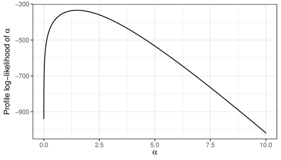
The plot of profile log-likelihood function, , is provided in the Figure 1. It is clear from the figure that the MLE of is near to 1.5. We take 1.5 as initial guess to implement iterative method to find the MLE of by maximizing (5). The point and interval estimates of the model parameter based on this dataset with order restriction on the scale parameters are reported in Table 9. Table 10 gives the point and interval estimates for the model parameters obtained based on this dataset when no restriction is imposed on the scale parameters.
7 Conclusion
In this article, we have discussed analysis of adaptive Type-II progressively censored competing risks data under order restriction on the scale parameters. The order restriction comes naturally if it is known that one risk factor dominates the other. The MLEs of the model parameters are derived, and parametric bootstrap confidence intervals are obtained. Bayes estimates of the model parameters are also derived, and construction of symmetric and highest posterior density credible intervals are discussed. Through an extensive Monte Carlo simulation study, the performance of the proposed methods are assessed. We also compare the performances of different estimators of different parameters under order restriction with those in unrestricted situation.
Through the simulation study, we observe that the Bayesian methods perform better than the classical methods at least for small samples under order restriction on the scale parameters. It is also noticed that the performances of estimators of scale parameter corresponding to lifetime of the non-dominating risk factor improve significantly when order restriction is used. The performances of the estimators of scale parameter corresponding to lifetime of the dominating risk factor are also improved. The performances of the estimators of the common shape parameter improve significantly under the order restriction for FSP, while for Type-II censoring or for OSP, the performances seem to be equivalent.
If we assume that the latent failure times have and distributions, respectively, under risk factors 1 and 2, it is quite difficult to find a necessary and sufficient condition such that the mean lifetime under risk factor 1 is less than that under risk factor 2. However, one may consider a sufficient condition on the parameters such that ordering on mean lifetimes holds true. One such sufficient condition can described as follows. Let us reparameterize as for . Then, and is a set of sufficient conditions. Under this conditions, the analysis can be performed in a similar way as described in Section 3.2. More work is needed along this direction.
| Likelihood Based | Bayesian | |||||||||||||
|---|---|---|---|---|---|---|---|---|---|---|---|---|---|---|
| Par | Bias | MSE | CPB | ALB | CPP | ALP | Bias | MSE | CPS | ALS | CPH | ALH | ||
| (0,…,0,10) | 0.25 | 0.07 | 0.055 | 0.956 | 0.91 | 0.920 | 0.90 | 0.05 | 0.052 | 0.944 | 0.83 | 0.947 | 0.82 | |
| 0.12 | 0.128 | 0.986 | 1.53 | 0.884 | 1.48 | 0.17 | 0.131 | 0.950 | 1.15 | 0.962 | 1.12 | |||
| 0.04 | 0.081 | 0.934 | 1.13 | 0.971 | 1.12 | -0.01 | 0.060 | 0.953 | 0.91 | 0.942 | 0.88 | |||
| -0.03 | 0.034 | 0.896 | 0.71 | 0.939 | 0.63 | -0.09 | 0.018 | 0.985 | 0.52 | 0.968 | 0.49 | |||
| 0.75 | 0.06 | 0.051 | 0.955 | 0.90 | 0.921 | 0.89 | 0.06 | 0.051 | 0.950 | 0.83 | 0.950 | 0.82 | ||
| 0.11 | 0.114 | 0.995 | 1.51 | 0.882 | 1.46 | 0.17 | 0.134 | 0.944 | 1.16 | 0.960 | 1.12 | |||
| 0.05 | 0.083 | 0.936 | 1.16 | 0.960 | 1.14 | -0.01 | 0.058 | 0.946 | 0.91 | 0.939 | 0.88 | |||
| -0.02 | 0.035 | 0.876 | 0.71 | 0.922 | 0.62 | -0.09 | 0.018 | 0.982 | 0.52 | 0.967 | 0.49 | |||
| (10,0,…,0) | 0.25 | 0.12 | 0.362 | 0.983 | 2.72 | 0.915 | 1.27 | 0.04 | 0.041 | 0.937 | 0.73 | 0.937 | 0.72 | |
| 0.08 | 0.093 | 0.982 | 1.46 | 0.915 | 1.27 | 0.13 | 0.089 | 0.942 | 0.98 | 0.951 | 0.95 | |||
| -0.00 | 0.062 | 0.944 | 1.05 | 0.957 | 1.01 | -0.04 | 0.043 | 0.928 | 0.78 | 0.918 | 0.76 | |||
| -0.03 | 0.032 | 0.910 | 0.71 | 0.946 | 0.62 | -0.09 | 0.018 | 0.982 | 0.52 | 0.966 | 0.49 | |||
| 0.75 | 0.12 | 0.394 | 0.992 | 2.80 | 0.908 | 1.31 | 0.04 | 0.038 | 0.948 | 0.73 | 0.943 | 0.72 | ||
| 0.06 | 0.093 | 0.979 | 1.35 | 0.911 | 1.27 | 0.13 | 0.088 | 0.942 | 0.99 | 0.948 | 0.95 | |||
| 0.00 | 0.057 | 0.943 | 1.04 | 0.961 | 1.01 | -0.04 | 0.042 | 0.935 | 0.78 | 0.924 | 0.76 | |||
| -0.02 | 0.033 | 0.908 | 0.71 | 0.944 | 0.62 | -0.09 | 0.019 | 0.982 | 0.52 | 0.967 | 0.49 | |||
| (0,…,10,…,0) | 0.25 | 0.05 | 0.051 | 0.976 | 0.91 | 0.931 | 0.89 | 0.06 | 0.053 | 0.944 | 0.83 | 0.946 | 0.82 | |
| 0.12 | 0.113 | 0.991 | 1.52 | 0.894 | 1.46 | 0.17 | 0.125 | 0.944 | 1.15 | 0.963 | 1.12 | |||
| 0.03 | 0.071 | 0.947 | 1.14 | 0.974 | 1.12 | -0.01 | 0.055 | 0.954 | 0.91 | 0.948 | 0.88 | |||
| -0.02 | 0.033 | 0.899 | 0.71 | 0.945 | 0.62 | -0.09 | 0.019 | 0.982 | 0.52 | 0.965 | 0.49 | |||
| 0.75 | 0.09 | 0.127 | 0.980 | 1.41 | 0.891 | 1.01 | 0.05 | 0.040 | 0.949 | 0.73 | 0.948 | 0.72 | ||
| 0.10 | 0.103 | 0.987 | 1.44 | 0.890 | 1.37 | 0.15 | 0.101 | 0.949 | 1.04 | 0.959 | 1.01 | |||
| 0.02 | 0.067 | 0.928 | 1.08 | 0.957 | 1.05 | -0.03 | 0.046 | 0.948 | 0.82 | 0.939 | 0.80 | |||
| -0.03 | 0.033 | 0.908 | 0.71 | 0.943 | 0.62 | -0.09 | 0.019 | 0.980 | 0.52 | 0.967 | 0.49 | |||
| Likelihood Based | Bayesian | |||||||||||||
|---|---|---|---|---|---|---|---|---|---|---|---|---|---|---|
| Par | Bias | MSE | CPB | ALB | CPP | ALP | Bias | MSE | CPS | ALS | CPH | ALH | ||
| (0,…,0,10) | 0.25 | 0.02 | 0.006 | 0.966 | 0.30 | 0.916 | 0.30 | 0.02 | 0.006 | 0.947 | 0.28 | 0.947 | 0.27 | |
| 0.12 | 0.117 | 0.989 | 1.53 | 0.879 | 1.48 | 0.16 | 0.125 | 0.951 | 1.15 | 0.959 | 1.10 | |||
| 0.05 | 0.072 | 0.950 | 1.16 | 0.975 | 1.14 | -0.01 | 0.055 | 0.959 | 0.90 | 0.949 | 0.87 | |||
| -0.02 | 0.032 | 0.904 | 0.71 | 0.950 | 0.62 | -0.09 | 0.018 | 0.989 | 0.52 | 0.974 | 0.49 | |||
| 0.75 | 0.02 | 0.006 | 0.961 | 0.30 | 0.922 | 0.30 | 0.02 | 0.006 | 0.942 | 0.28 | 0.943 | 0.27 | ||
| 0.12 | 0.126 | 0.991 | 1.54 | 0.867 | 1.49 | 0.16 | 0.124 | 0.950 | 1.15 | 0.963 | 1.11 | |||
| 0.03 | 0.070 | 0.939 | 1.15 | 0.961 | 1.13 | -0.01 | 0.055 | 0.952 | 0.90 | 0.943 | 0.87 | |||
| -0.03 | 0.034 | 0.887 | 0.71 | 0.936 | 0.62 | -0.09 | 0.019 | 0.984 | 0.52 | 0.970 | 0.49 | |||
| (10,0,…,0) | 0.25 | 0.04 | 0.041 | 0.993 | 0.92 | 0.901 | 0.37 | 0.02 | 0.004 | 0.952 | 0.25 | 0.950 | 0.24 | |
| 0.09 | 0.100 | 0.981 | 1.39 | 0.908 | 1.29 | 0.13 | 0.084 | 0.952 | 0.99 | 0.960 | 0.96 | |||
| 0.01 | 0.064 | 0.934 | 1.05 | 0.948 | 1.02 | -0.03 | 0.040 | 0.952 | 0.79 | 0.940 | 0.77 | |||
| -0.03 | 0.033 | 0.893 | 0.71 | 0.934 | 0.62 | -0.09 | 0.018 | 0.987 | 0.52 | 0.967 | 0.49 | |||
| 0.75 | 0.04 | 0.052 | 0.996 | 0.95 | 0.914 | 0.38 | 0.02 | 0.004 | 0.944 | 0.25 | 0.945 | 0.24 | ||
| 0.07 | 0.103 | 0.984 | 1.44 | 0.926 | 1.29 | 0.13 | 0.087 | 0.945 | 0.99 | 0.956 | 0.96 | |||
| 0.01 | 0.073 | 0.948 | 1.11 | 0.952 | 1.01 | -0.03 | 0.042 | 0.951 | 0.79 | 0.937 | 0.77 | |||
| -0.02 | 0.033 | 0.911 | 0.71 | 0.945 | 0.62 | -0.09 | 0.018 | 0.984 | 0.52 | 0.968 | 0.49 | |||
| (0,…,10,…,0) | 0.25 | 0.03 | 0.012 | 0.986 | 0.46 | 0.887 | 0.36 | 0.01 | 0.004 | 0.946 | 0.24 | 0.946 | 0.24 | |
| 0.10 | 0.103 | 0.990 | 1.46 | 0.893 | 1.38 | 0.15 | 0.101 | 0.950 | 1.04 | 0.957 | 1.01 | |||
| 0.04 | 0.071 | 0.941 | 1.11 | 0.947 | 1.08 | -0.03 | 0.045 | 0.947 | 0.83 | 0.937 | 0.81 | |||
| -0.02 | 0.033 | 0.907 | 0.71 | 0.939 | 0.62 | -0.09 | 0.019 | 0.983 | 0.52 | 0.964 | 0.49 | |||
| 0.75 | 0.04 | 0.017 | 0.983 | 0.47 | 0.877 | 0.37 | 0.02 | 0.004 | 0.949 | 0.24 | 0.949 | 0.24 | ||
| 0.11 | 0.112 | 0.984 | 1.46 | 0.881 | 1.38 | 0.14 | 0.101 | 0.947 | 1.04 | 0.957 | 1.01 | |||
| 0.04 | 0.073 | 0.933 | 1.12 | 0.949 | 1.08 | -0.02 | 0.045 | 0.953 | 0.83 | 0.940 | 0.81 | |||
| -0.02 | 0.032 | 0.899 | 0.71 | 0.935 | 0.62 | -0.09 | 0.018 | 0.988 | 0.52 | 0.971 | 0.49 | |||
| Likelihood Based | Bayesian | |||||||||||||
|---|---|---|---|---|---|---|---|---|---|---|---|---|---|---|
| Par | Bias | MSE | CPB | ALB | CPP | ALP | Bias | MSE | CPS | ALS | CPH | ALH | ||
| (0,…,0,10) | 0.25 | 0.07 | 0.057 | 0.958 | 0.90 | 0.918 | 0.89 | 0.06 | 0.051 | 0.946 | 0.83 | 0.945 | 0.82 | |
| 0.11 | 0.167 | 0.976 | 1.77 | 0.917 | 1.71 | 0.15 | 0.156 | 0.957 | 1.36 | 0.962 | 1.31 | |||
| 0.06 | 0.099 | 0.945 | 1.27 | 0.967 | 1.25 | 0.03 | 0.069 | 0.964 | 1.01 | 0.957 | 0.99 | |||
| 0.00 | 0.036 | 0.929 | 0.71 | 0.964 | 0.63 | -0.02 | 0.014 | 0.988 | 0.56 | 0.971 | 0.53 | |||
| 0.75 | 0.06 | 0.052 | 0.964 | 0.90 | 0.919 | 0.89 | 0.06 | 0.052 | 0.946 | 0.83 | 0.946 | 0.82 | ||
| 0.13 | 0.182 | 0.985 | 1.81 | 0.897 | 1.75 | 0.16 | 0.175 | 0.949 | 1.38 | 0.959 | 1.33 | |||
| 0.05 | 0.092 | 0.944 | 1.27 | 0.969 | 1.24 | 0.04 | 0.076 | 0.959 | 1.02 | 0.955 | 1.00 | |||
| 0.01 | 0.038 | 0.925 | 0.70 | 0.962 | 0.63 | -0.02 | 0.014 | 0.988 | 0.56 | 0.972 | 0.53 | |||
| (10,0,…,0) | 0.25 | 0.14 | 0.504 | 0.980 | 2.72 | 0.913 | 1.12 | 0.05 | 0.039 | 0.946 | 0.73 | 0.944 | 0.72 | |
| 0.07 | 0.136 | 0.971 | 1.58 | 0.924 | 1.47 | 0.11 | 0.105 | 0.956 | 1.16 | 0.956 | 1.12 | |||
| 0.03 | 0.082 | 0.939 | 1.15 | 0.955 | 1.11 | 0.01 | 0.052 | 0.955 | 0.88 | 0.948 | 0.86 | |||
| 0.01 | 0.038 | 0.920 | 0.70 | 0.962 | 0.63 | -0.02 | 0.014 | 0.987 | 0.56 | 0.974 | 0.53 | |||
| 0.75 | 0.14 | 0.484 | 0.993 | 2.83 | 0.905 | 1.12 | 0.05 | 0.040 | 0.950 | 0.73 | 0.949 | 0.72 | ||
| 0.08 | 0.148 | 0.979 | 1.63 | 0.916 | 1.49 | 0.11 | 0.107 | 0.948 | 1.16 | 0.952 | 1.12 | |||
| 0.03 | 0.079 | 0.948 | 1.15 | 0.957 | 1.11 | 0.01 | 0.052 | 0.952 | 0.88 | 0.946 | 0.86 | |||
| -0.00 | 0.037 | 0.924 | 0.70 | 0.967 | 0.63 | -0.02 | 0.014 | 0.988 | 0.56 | 0.974 | 0.53 | |||
| (0,…,10,…,0) | 0.25 | 0.06 | 0.049 | 0.975 | 0.93 | 0.923 | 0.90 | 0.06 | 0.051 | 0.947 | 0.83 | 0.946 | 0.82 | |
| 0.11 | 0.163 | 0.978 | 1.81 | 0.913 | 1.74 | 0.14 | 0.166 | 0.954 | 1.35 | 0.962 | 1.31 | |||
| 0.07 | 0.109 | 0.956 | 1.30 | 0.964 | 1.27 | 0.04 | 0.074 | 0.961 | 1.01 | 0.953 | 0.99 | |||
| 0.01 | 0.037 | 0.923 | 0.71 | 0.960 | 0.63 | -0.02 | 0.014 | 0.990 | 0.56 | 0.979 | 0.53 | |||
| 0.75 | 0.09 | 0.109 | 0.989 | 1.37 | 0.904 | 1.09 | 0.05 | 0.040 | 0.946 | 0.73 | 0.946 | 0.72 | ||
| 0.10 | 0.144 | 0.980 | 1.68 | 0.923 | 1.59 | 0.12 | 0.131 | 0.952 | 1.23 | 0.957 | 1.19 | |||
| 0.06 | 0.098 | 0.952 | 1.25 | 0.958 | 1.20 | 0.02 | 0.062 | 0.956 | 0.93 | 0.947 | 0.90 | |||
| 0.00 | 0.038 | 0.928 | 0.70 | 0.960 | 0.63 | -0.02 | 0.015 | 0.985 | 0.56 | 0.971 | 0.53 | |||
| Likelihood Based | Bayesian | |||||||||||||
|---|---|---|---|---|---|---|---|---|---|---|---|---|---|---|
| Par | Bias | MSE | CPB | ALB | CPP | ALP | Bias | MSE | CPS | ALS | CPH | ALH | ||
| (0,…,0,10) | 0.25 | 0.02 | 0.006 | 0.968 | 0.30 | 0.920 | 0.30 | 0.02 | 0.006 | 0.947 | 0.28 | 0.947 | 0.27 | |
| 0.11 | 0.149 | 0.981 | 1.78 | 0.922 | 1.71 | 0.15 | 0.166 | 0.954 | 1.37 | 0.962 | 1.31 | |||
| 0.06 | 0.086 | 0.956 | 1.27 | 0.965 | 1.25 | 0.04 | 0.072 | 0.963 | 1.02 | 0.961 | 0.99 | |||
| 0.01 | 0.038 | 0.919 | 0.70 | 0.956 | 0.63 | -0.02 | 0.014 | 0.989 | 0.56 | 0.977 | 0.53 | |||
| 0.75 | 0.02 | 0.006 | 0.952 | 0.30 | 0.921 | 0.30 | 0.02 | 0.006 | 0.947 | 0.28 | 0.947 | 0.27 | ||
| 0.11 | 0.163 | 0.980 | 1.78 | 0.902 | 1.71 | 0.15 | 0.160 | 0.956 | 1.37 | 0.959 | 1.31 | |||
| 0.06 | 0.102 | 0.949 | 1.27 | 0.956 | 1.25 | 0.04 | 0.072 | 0.960 | 1.02 | 0.956 | 0.99 | |||
| 0.01 | 0.038 | 0.922 | 0.70 | 0.959 | 0.63 | -0.02 | 0.014 | 0.989 | 0.56 | 0.975 | 0.53 | |||
| (10,0,…,0) | 0.25 | 0.05 | 0.054 | 0.989 | 0.93 | 0.904 | 0.38 | 0.01 | 0.004 | 0.948 | 0.24 | 0.948 | 0.24 | |
| 0.07 | 0.139 | 0.977 | 1.74 | 0.919 | 1.47 | 0.11 | 0.099 | 0.961 | 1.16 | 0.965 | 1.12 | |||
| 0.03 | 0.084 | 0.938 | 1.26 | 0.947 | 1.11 | 0.01 | 0.048 | 0.970 | 0.89 | 0.962 | 0.87 | |||
| 0.01 | 0.038 | 0.919 | 0.70 | 0.954 | 0.63 | -0.02 | 0.014 | 0.990 | 0.56 | 0.975 | 0.53 | |||
| 0.75 | 0.05 | 0.044 | 0.995 | 0.96 | 0.892 | 0.37 | 0.02 | 0.004 | 0.952 | 0.25 | 0.953 | 0.24 | ||
| 0.07 | 0.134 | 0.973 | 1.61 | 0.922 | 1.48 | 0.11 | 0.108 | 0.956 | 1.16 | 0.956 | 1.13 | |||
| 0.04 | 0.078 | 0.953 | 1.17 | 0.965 | 1.12 | 0.01 | 0.051 | 0.961 | 0.89 | 0.953 | 0.87 | |||
| 0.01 | 0.036 | 0.930 | 0.71 | 0.969 | 0.63 | -0.02 | 0.014 | 0.991 | 0.56 | 0.977 | 0.53 | |||
| (0,…,10,…,0) | 0.25 | 0.03 | 0.011 | 0.987 | 0.46 | 0.906 | 0.36 | 0.02 | 0.004 | 0.946 | 0.24 | 0.946 | 0.24 | |
| 0.10 | 0.142 | 0.974 | 1.72 | 0.909 | 1.61 | 0.12 | 0.128 | 0.952 | 1.22 | 0.954 | 1.18 | |||
| 0.04 | 0.080 | 0.949 | 1.23 | 0.965 | 1.18 | 0.02 | 0.059 | 0.956 | 0.93 | 0.952 | 0.90 | |||
| 0.00 | 0.037 | 0.917 | 0.70 | 0.957 | 0.63 | -0.02 | 0.014 | 0.989 | 0.55 | 0.975 | 0.53 | |||
| 0.75 | 0.03 | 0.012 | 0.989 | 0.46 | 0.897 | 0.36 | 0.02 | 0.004 | 0.954 | 0.24 | 0.951 | 0.24 | ||
| 0.11 | 0.142 | 0.978 | 1.71 | 0.897 | 1.60 | 0.12 | 0.123 | 0.953 | 1.22 | 0.958 | 1.18 | |||
| 0.05 | 0.081 | 0.944 | 1.23 | 0.958 | 1.18 | 0.02 | 0.058 | 0.959 | 0.93 | 0.955 | 0.90 | |||
| 0.00 | 0.037 | 0.921 | 0.70 | 0.952 | 0.63 | -0.02 | 0.014 | 0.988 | 0.56 | 0.976 | 0.53 | |||
| Likelihood Based | Bayesian | |||||||||||||
|---|---|---|---|---|---|---|---|---|---|---|---|---|---|---|
| Par | Bias | MSE | CPB | ALB | CPP | ALP | Bias | MSE | CPS | ALS | CPH | ALH | ||
| (0,…,0,10) | 0.25 | 0.06 | 0.051 | 0.964 | 0.90 | 0.914 | 0.89 | 0.06 | 0.054 | 0.943 | 0.83 | 0.946 | 0.83 | |
| 0.08 | 0.119 | 0.965 | 1.47 | 0.940 | 1.43 | 0.09 | 0.131 | 0.944 | 1.23 | 0.948 | 1.19 | |||
| 0.06 | 0.094 | 0.965 | 1.31 | 0.936 | 1.28 | 0.08 | 0.106 | 0.938 | 1.10 | 0.938 | 1.07 | |||
| 0.75 | 0.06 | 0.049 | 0.966 | 0.90 | 0.932 | 0.89 | 0.05 | 0.049 | 0.950 | 0.83 | 0.948 | 0.82 | ||
| 0.09 | 0.115 | 0.963 | 1.50 | 0.934 | 1.48 | 0.08 | 0.118 | 0.943 | 1.22 | 0.946 | 1.18 | |||
| 0.08 | 0.094 | 0.964 | 1.33 | 0.922 | 1.30 | 0.06 | 0.093 | 0.946 | 1.09 | 0.944 | 1.05 | |||
| (10,0,…,0) | 0.25 | 0.10 | 0.339 | 0.990 | 2.76 | 0.919 | 1.11 | 0.05 | 0.040 | 0.947 | 0.73 | 0.944 | 0.72 | |
| 0.06 | 0.112 | 0.961 | 1.30 | 0.937 | 1.26 | 0.05 | 0.092 | 0.941 | 1.08 | 0.937 | 1.05 | |||
| 0.04 | 0.085 | 0.954 | 1.16 | 0.934 | 1.13 | 0.04 | 0.076 | 0.940 | 0.98 | 0.932 | 0.95 | |||
| 0.75 | 0.12 | 0.292 | 0.996 | 2.84 | 0.898 | 1.16 | 0.04 | 0.040 | 0.941 | 0.73 | 0.939 | 0.72 | ||
| 0.06 | 0.095 | 0.966 | 1.33 | 0.945 | 1.27 | 0.04 | 0.089 | 0.945 | 1.07 | 0.938 | 1.04 | |||
| 0.05 | 0.083 | 0.959 | 1.18 | 0.937 | 1.14 | 0.05 | 0.074 | 0.940 | 0.98 | 0.937 | 0.95 | |||
| (0,…,10,…,0) | 0.25 | 0.06 | 0.057 | 0.963 | 0.92 | 0.909 | 0.90 | 0.06 | 0.053 | 0.947 | 0.83 | 0.948 | 0.83 | |
| 0.11 | 0.134 | 0.976 | 1.49 | 0.928 | 1.48 | 0.09 | 0.126 | 0.949 | 1.23 | 0.952 | 1.20 | |||
| 0.07 | 0.107 | 0.958 | 1.31 | 0.916 | 1.28 | 0.07 | 0.099 | 0.943 | 1.10 | 0.940 | 1.07 | |||
| 0.75 | 0.08 | 0.121 | 0.988 | 1.38 | 0.885 | 1.05 | 0.05 | 0.040 | 0.949 | 0.73 | 0.947 | 0.72 | ||
| 0.06 | 0.106 | 0.959 | 1.42 | 0.940 | 1.37 | 0.06 | 0.099 | 0.944 | 1.12 | 0.942 | 1.09 | |||
| 0.08 | 0.094 | 0.968 | 1.25 | 0.932 | 1.21 | 0.05 | 0.082 | 0.943 | 1.01 | 0.941 | 0.98 | |||
| Likelihood Based | Bayesian | |||||||||||||
|---|---|---|---|---|---|---|---|---|---|---|---|---|---|---|
| Par | Bias | MSE | CPB | ALB | CPP | ALP | Bias | MSE | CPS | ALS | CPH | ALH | ||
| (0,…,0,10) | 0.25 | 0.02 | 0.006 | 0.965 | 0.30 | 0.920 | 0.29 | 0.02 | 0.006 | 0.941 | 0.28 | 0.940 | 0.28 | |
| 0.07 | 0.114 | 0.965 | 1.45 | 0.931 | 1.42 | 0.09 | 0.122 | 0.946 | 1.23 | 0.949 | 1.19 | |||
| 0.07 | 0.092 | 0.966 | 1.30 | 0.931 | 1.27 | 0.07 | 0.100 | 0.945 | 1.10 | 0.940 | 1.06 | |||
| 0.75 | 0.02 | 0.006 | 0.956 | 0.30 | 0.923 | 0.30 | 0.02 | 0.006 | 0.949 | 0.28 | 0.951 | 0.27 | ||
| 0.09 | 0.118 | 0.965 | 1.49 | 0.937 | 1.46 | 0.08 | 0.117 | 0.952 | 1.22 | 0.948 | 1.18 | |||
| 0.07 | 0.090 | 0.964 | 1.32 | 0.937 | 1.29 | 0.07 | 0.091 | 0.948 | 1.09 | 0.945 | 1.05 | |||
| (10,0,…,0) | 0.25 | 0.05 | 0.083 | 0.986 | 0.93 | 0.906 | 0.38 | 0.01 | 0.004 | 0.949 | 0.24 | 0.948 | 0.24 | |
| 0.05 | 0.115 | 0.953 | 1.34 | 0.940 | 1.29 | 0.05 | 0.091 | 0.946 | 1.08 | 0.939 | 1.06 | |||
| 0.04 | 0.092 | 0.954 | 1.19 | 0.939 | 1.16 | 0.04 | 0.072 | 0.943 | 0.98 | 0.942 | 0.96 | |||
| 0.75 | 0.06 | 0.107 | 0.990 | 0.95 | 0.899 | 0.38 | 0.01 | 0.004 | 0.948 | 0.25 | 0.950 | 0.24 | ||
| 0.05 | 0.118 | 0.960 | 1.33 | 0.929 | 1.28 | 0.04 | 0.085 | 0.946 | 1.07 | 0.941 | 1.05 | |||
| 0.03 | 0.093 | 0.942 | 1.17 | 0.929 | 1.14 | 0.05 | 0.070 | 0.946 | 0.98 | 0.943 | 0.96 | |||
| (0,…,10,…,0) | 0.25 | 0.03 | 0.013 | 0.982 | 0.46 | 0.906 | 0.36 | 0.01 | 0.004 | 0.947 | 0.24 | 0.950 | 0.24 | |
| 0.06 | 0.108 | 0.953 | 1.40 | 0.929 | 1.35 | 0.06 | 0.099 | 0.946 | 1.12 | 0.943 | 1.09 | |||
| 0.05 | 0.086 | 0.954 | 1.24 | 0.934 | 1.20 | 0.05 | 0.076 | 0.945 | 1.01 | 0.939 | 0.98 | |||
| 0.75 | 0.03 | 0.014 | 0.983 | 0.46 | 0.910 | 0.36 | 0.02 | 0.004 | 0.948 | 0.24 | 0.949 | 0.24 | ||
| 0.05 | 0.097 | 0.957 | 1.41 | 0.938 | 1.36 | 0.06 | 0.100 | 0.949 | 1.13 | 0.945 | 1.10 | |||
| 0.05 | 0.081 | 0.953 | 1.26 | 0.931 | 1.23 | 0.06 | 0.083 | 0.943 | 1.02 | 0.938 | 0.99 | |||
| Likelihood Based | Bayesian | |||||||||||||
|---|---|---|---|---|---|---|---|---|---|---|---|---|---|---|
| Par | Bias | MSE | CPB | ALB | CPP | ALP | Bias | MSE | CPS | ALS | CPH | ALH | ||
| (0,…,0,10) | 0.25 | 0.06 | 0.053 | 0.968 | 0.90 | 0.919 | 0.89 | 0.055 | 0.052 | 0.947 | 0.83 | 0.950 | 0.82 | |
| 0.11 | 0.186 | 0.965 | 1.78 | 0.913 | 1.74 | 0.116 | 0.180 | 0.944 | 1.45 | 0.945 | 1.41 | |||
| 0.09 | 0.115 | 0.969 | 1.43 | 0.935 | 1.40 | 0.082 | 0.111 | 0.945 | 1.17 | 0.947 | 1.13 | |||
| 0.75 | 0.05 | 0.047 | 0.967 | 0.90 | 0.930 | 0.89 | 0.055 | 0.052 | 0.948 | 0.83 | 0.946 | 0.82 | ||
| 0.08 | 0.148 | 0.964 | 1.73 | 0.934 | 1.68 | 0.111 | 0.183 | 0.947 | 1.44 | 0.949 | 1.40 | |||
| 0.07 | 0.101 | 0.960 | 1.38 | 0.933 | 1.35 | 0.081 | 0.115 | 0.948 | 1.17 | 0.948 | 1.13 | |||
| (10,0,…,0) | 0.25 | 0.13 | 0.455 | 0.984 | 2.73 | 0.916 | 1.10 | 0.040 | 0.039 | 0.945 | 0.73 | 0.944 | 0.72 | |
| 0.06 | 0.138 | 0.967 | 1.59 | 0.933 | 1.50 | 0.069 | 0.123 | 0.944 | 1.25 | 0.945 | 1.21 | |||
| 0.04 | 0.095 | 0.949 | 1.27 | 0.937 | 1.22 | 0.044 | 0.084 | 0.936 | 1.03 | 0.932 | 1.00 | |||
| 0.75 | 0.12 | 0.408 | 0.996 | 2.83 | 0.899 | 1.11 | 0.043 | 0.040 | 0.942 | 0.73 | 0.943 | 0.72 | ||
| 0.07 | 0.137 | 0.969 | 1.59 | 0.940 | 1.50 | 0.064 | 0.120 | 0.941 | 1.24 | 0.941 | 1.21 | |||
| 0.04 | 0.083 | 0.962 | 1.26 | 0.951 | 1.21 | 0.047 | 0.083 | 0.940 | 1.03 | 0.935 | 1.00 | |||
| (0,…,10,…,0) | 0.25 | 0.06 | 0.049 | 0.982 | 0.92 | 0.929 | 0.89 | 0.060 | 0.054 | 0.942 | 0.83 | 0.944 | 0.83 | |
| 0.09 | 0.168 | 0.971 | 1.75 | 0.936 | 1.70 | 0.114 | 0.181 | 0.946 | 1.45 | 0.947 | 1.40 | |||
| 0.07 | 0.104 | 0.959 | 1.40 | 0.938 | 1.36 | 0.086 | 0.120 | 0.941 | 1.17 | 0.941 | 1.13 | |||
| 0.75 | 0.10 | 0.118 | 0.985 | 1.40 | 0.886 | 1.11 | 0.047 | 0.039 | 0.946 | 0.73 | 0.948 | 0.72 | ||
| 0.10 | 0.146 | 0.969 | 1.71 | 0.929 | 1.63 | 0.079 | 0.138 | 0.948 | 1.30 | 0.946 | 1.27 | |||
| 0.07 | 0.088 | 0.968 | 1.36 | 0.941 | 1.30 | 0.059 | 0.089 | 0.946 | 1.08 | 0.944 | 1.04 | |||
| Likelihood Based | Bayesian | |||||||||||||
|---|---|---|---|---|---|---|---|---|---|---|---|---|---|---|
| Par | Bias | MSE | CPB | ALB | CPP | ALP | Bias | MSE | CPS | ALS | CPH | ALH | ||
| (0,…,0,10) | 0.25 | 0.02 | 0.006 | 0.966 | 0.30 | 0.927 | 0.30 | 0.021 | 0.006 | 0.949 | 0.28 | 0.952 | 0.28 | |
| 0.11 | 0.175 | 0.968 | 1.78 | 0.918 | 1.73 | 0.117 | 0.175 | 0.949 | 1.45 | 0.949 | 1.40 | |||
| 0.07 | 0.109 | 0.954 | 1.41 | 0.942 | 1.38 | 0.078 | 0.109 | 0.949 | 1.17 | 0.944 | 1.12 | |||
| 0.75 | 0.02 | 0.006 | 0.962 | 0.30 | 0.909 | 0.30 | 0.020 | 0.006 | 0.949 | 0.28 | 0.949 | 0.28 | ||
| 0.11 | 0.159 | 0.964 | 1.78 | 0.937 | 1.73 | 0.114 | 0.178 | 0.941 | 1.44 | 0.944 | 1.40 | |||
| 0.08 | 0.115 | 0.957 | 1.42 | 0.933 | 1.38 | 0.077 | 0.108 | 0.948 | 1.17 | 0.944 | 1.12 | |||
| (10,0,…,0) | 0.25 | 0.04 | 0.028 | 0.995 | 0.92 | 0.904 | 0.37 | 0.017 | 0.005 | 0.942 | 0.25 | 0.945 | 0.24 | |
| 0.06 | 0.131 | 0.964 | 1.60 | 0.938 | 1.50 | 0.068 | 0.122 | 0.949 | 1.25 | 0.945 | 1.22 | |||
| 0.05 | 0.099 | 0.953 | 1.28 | 0.926 | 1.23 | 0.046 | 0.080 | 0.947 | 1.04 | 0.941 | 1.01 | |||
| 0.75 | 0.05 | 0.055 | 0.993 | 0.95 | 0.903 | 0.38 | 0.016 | 0.004 | 0.947 | 0.25 | 0.948 | 0.24 | ||
| 0.06 | 0.140 | 0.955 | 1.56 | 0.936 | 1.49 | 0.061 | 0.120 | 0.941 | 1.25 | 0.936 | 1.22 | |||
| 0.03 | 0.091 | 0.944 | 1.25 | 0.936 | 1.21 | 0.048 | 0.080 | 0.945 | 1.04 | 0.939 | 1.01 | |||
| (0,…,10,…,0) | 0.25 | 0.03 | 0.012 | 0.986 | 0.46 | 0.890 | 0.37 | 0.016 | 0.004 | 0.946 | 0.24 | 0.948 | 0.24 | |
| 0.10 | 0.160 | 0.965 | 1.72 | 0.928 | 1.64 | 0.071 | 0.133 | 0.947 | 1.30 | 0.943 | 1.26 | |||
| 0.07 | 0.092 | 0.969 | 1.37 | 0.939 | 1.31 | 0.055 | 0.086 | 0.947 | 1.07 | 0.943 | 1.04 | |||
| 0.75 | 0.03 | 0.018 | 0.984 | 0.47 | 0.906 | 0.37 | 0.015 | 0.005 | 0.937 | 0.24 | 0.938 | 0.24 | ||
| 0.08 | 0.143 | 0.963 | 1.69 | 0.929 | 1.60 | 0.084 | 0.146 | 0.939 | 1.31 | 0.941 | 1.28 | |||
| 0.06 | 0.090 | 0.956 | 1.34 | 0.935 | 1.28 | 0.056 | 0.090 | 0.948 | 1.08 | 0.943 | 1.04 | |||
| Likelihood | Bayesian | |||||
|---|---|---|---|---|---|---|
| Parameter | MLE | BB | PB | BE | SCRI | HPD CRI |
| 1.49 | (1.22, 1.72) | (1.30, 1.81) | 1.49 | (1.26, 1.75) | (1.27, 1.76) | |
| 1.62 | (1.11, 2.04) | (1.23, 2.16) | 1.58 | (1.19, 2.06) | (1.19, 2.04) | |
| 0.89 | (0.53, 1.20) | (0.62, 1.27) | 0.91 | (0.64, 1.26) | (0.61, 1.22) | |
| Likelihood | Bayesian | |||||
|---|---|---|---|---|---|---|
| Parameter | MLE | BB | PB | BE | SCRI | HPD CRI |
| 1.49 | (1.23, 1.73) | (1.286, 1.770) | 1.49 | (1.26, 1.74) | (1.25, 1.72) | |
| 1.62 | (1.13, 2.05) | (1.213, 2.125) | 1.61 | (1.20, 2.09) | (1.18, 2.05) | |
| 0.89 | (0.52, 1.20) | (0.605, 1.283) | 0.89 | (0.60, 1.24) | (0.60, 1.23) | |
Acknowledgements
The research of Ayon Ganguly is supported by the Mathematical Research Impact
Centric Support (File no. MTR/2017/000700) from the Science and
Engineering Research Board, Department of Science and Technology, Government of
India.
Debanjan Mitra thanks Indian Institute of Management Udaipur for financial
support to carry out this research.
References
- [1] Balakrishnan, N., Beutner, E., and Kateri, M. Order restricted inference for exponential step-stress models. IEEE Transactions on Reliability 58 (2009), 132–142.
- [2] Balakrishnan, N., and Cramer, E. The art of Progressive censoring: applications to reliability and quality. Birkhäuser, Boston, 2014.
- [3] Berger, J. O., and Sun, D. Bayesian analysis for the Poly-Weibull distribution. Journal of American Statistical Association 88 (1993), 1412–1418.
- [4] Burkschat, M. On optimality of extremal schemes in progressive type II censoring. Journal of Statistical Planning and Inference (2008), 1647–1659.
- [5] Cox, D. R. The analysis of exponentially distributed lifetimes with two types of failures. Journal of the Royal Statistical Society, Series B 21 (1959), 411–421.
- [6] David, H. A., and Nagaraja, H. N. Order statistics, 3 ed. John Wiley and Sons, New York, 2003.
- [7] Kundu, D. Parameter estimation of the partially complete time and type of failure data. Biometrical Journal 46 (2004), 165–179.
- [8] Kundu, D. Bayesian inference and life testing plan for Weibull distribution in presence of progressive censoring. Technometrics 50 (2008), 144–154.
- [9] Kundu, D., and Gupta, R. Estimation of for Weibull distribution. IEEE Transactions on Reliability 55 (2006), 270–280.
- [10] Mahto, A., Lodhi, C., Tripathi, Y., and Wang, L. Inference for partially observed competing risks model for Kumaraswamy distribution under generalized progressive hybrid censoring. Journal of Applied Statistics (2021).
- [11] Ng, H. K. T., Chan, P. S., and Balakrishnan, N. Optimum progressive censoring plan for the Weibull distribution. Technometrics 46 (2004), 470–481.
- [12] Ng, H. K. T., Kundu, D., and Chan, P. S. Statistical analysis of exponential lifetimes under an adaptive Type-II progressive censoring scheme. Naval Research Logistics 56 (2009), 687–698.
- [13] Pal, A., Mitra, S., and Kundu, D. Bayesian order restricted inference of a weibull multi-step step-stress model. Journal of Statistical Theory and Practice 15 (2021).
- [14] Pal, A., Mitra, S., and Kundu, D. Order restricted classical inference of a weibull multiple step-stress model. Journal of Applied Statistics 48 (2021), 623 –645.
- [15] Pareek, B., Kundu, D., and Kumar, S. On progressively censored competing risks data for Weibull distributions. Computational Statistics and Data Analysis 53 (2009), 4083–4094.
- [16] Pascual, F. Accelerated life test planning with independent Weibull competing risks with known shape parameter. IEEE Transactions on Reliability 56 (2007), 85–93.
- [17] Pascual, F. Accelerated life test planning with independent Weibull competing risks. IEEE Transactions on Reliability 57 (2008), 435–444.
- [18] Prentice, R. L., Kalbfleish, J., Peterson, J. A., Flurnoy, N., Farewell, V. T., and Breslow, N. The analysis of failure time points in presence of competing risks. Biometrics 34 (1978), 541 – 544.
- [19] Ren, J., and Gui, W. Statistical analysis of adaptive type-II progressively censored competing risks for Weibull moels. Applied Mathematical Modelling 98 (2021), 323–342.
- [20] Samanta, D., Ganguly, A., Kundu, D., and Mitra, S. Order restricted Bayesian inference for exponential simple step-stress model. Communication in Statistics - Simulation and Computation 46 (2017), 1113–1135.