Ordering Behavior of the Two-Dimensional Ising Spin Glass with Long-Range Correlated Disorder
Abstract
The standard two-dimensional Ising spin glass does not exhibit an ordered phase at finite temperature. Here, we investigate whether long-range correlated bonds change this behavior. The bonds are drawn from a Gaussian distribution with a two-point correlation for bonds at distance that decays as , . We study numerically with exact algorithms the ground state and domain wall excitations. Our results indicate that the inclusion of bond correlations does not lead to a spin-glass order at any finite temperature. A further analysis reveals that bond correlations have a strong effect at local length scales, inducing ferro/antiferromagnetic domains into the system. The length scale of ferro/antiferromagnetic order diverges exponentially as the correlation exponent approaches a critical value, . Thus, our results suggest that the system becomes a ferro/antiferromagnet only in the limit .
pacs:
75.40.Mg, 02.60.Pn, 68.35.RhI Introduction
Spin glasses are disordered magnetic materials which exhibit peculiar properties at very low temperatures Vincent and Dupuis (2018). To understand these materials, the Edwards-Anderson (EA) model and the Sherrington-Kirkpatrick (SK) model Edwards and Anderson (1975); Sherrington and Kirkpatrick (1975) have been developed. Spin glasses exhibit essential aspects of complex behavior Stein and Newman (2013) and research on spin glasses Mézard et al. (1987); Young (1998); Bolthausen and Bovier (2007) has stimulated progress in numerous other fields, such as information processing Nishimori (2001), neuronal networks Dotsenko (1994), discrete optimization Hartmann and Rieger (2002, 2004) and Monte-Carlo simulation Zhu et al. (2015).
In this work we study the two-dimensional EA spin glass model with Ising spins. This model has short-range quenched random pair-wise interactions, described in detail in Sec. II. Its properties are well described in the framework of the scaling/droplet picture McMillan (1984); Bray and Moore (1987a); Fisher and Huse (1988), as has been confirmed by numerical calculations for large systems using exact ground-state algorithms Hartmann and Moore (2003, 2004). The model exhibits no finite-temperature spin glass phas,e in contrast to the three or higher dimensional variants Young and Stinchcombe (1976); Southern and Young (1977); Hartmann and Young (2001).
At the zero-temperature phase transition, the distribution of the interaction disorder, in particular differences between continuous Gaussian and discrete bimodal disorder distributions have been the subject of intensive research Khoshbakht and Weigel (2018); Parisen Toldin et al. (2011); Thomas et al. (2011); Fernandez et al. (2016). Since the non-existence of a finite-temperature spin-glass phase for short range two-dimensional models is independent of the disorder distribution, we consider here only the Gaussian case. Previous works have shown how the increase of the mean of the Gaussian from zero to a sufficiently large value induces a ferromagnetic phase Sherrington and Southern (1975); Amoruso and Hartmann (2004); Fisch and Hartmann (2007); Monthus and Garel (2014); Fajen et al. (2020).
In this work we address the question how long-range correlations in the interactions (bonds) affects the ordering behavior, in particular whether it leads to a low-temperature spin-glass phase. Here, long-range means that the bond correlation decays with a power law and so does not have a characteristic length scale. For disordered ferromagnets the effects of long-range correlations have already been taken studied Weinrib and Halperin (1983).
Our study was partially motivated by a corresponding numerical study of the three-dimensional random-field Ising model with long-range correlation Ahrens and Hartmann (2011), where, for strong correlation, an influence on the quantitative ordering behavior has been observed for some critical exponents. Note, however, that the case of the random-field model is a bit different, because the correlation acts on the random fields which provide local randomness competing against long-range ferromagnetic order. Consequently, from an extended Imry-Ma argument it was predicted Nattermann (1998) that the random-field Ising model with strong long-range correlation will show an increase of the lower critical dimension for ferromagnetic order. We note that there is no analogous prediction for the spin-glass case.
The following content is structured into three parts. First, the model is introduced and it is outlined how ground state computations under changing boundary conditions are used to produce domain wall excitations. Second, the results of the simulations will be presented. Finally we give a discussion.
II Model and Methods
II.1 The Ising Spin Glass with Correlated Bonds
The Ising spin glass consist of Ising spins on the sites of a two-dimensional lattice, i.e. . In this study only square systems are considered, such that the spin glass has spins in each direction and . The Hamiltonian is given by
| (1) |
where the sum runs over all pairs of nearest-neighbor spin sites with periodic boundary conditions (BC) in one and free boundary conditions in the other direction. The bonds, , which represent the interaction between two spins, are random in strength and sign but remain constant over time. Hence, one speaks of a quenched disorder where the system is investigated under a fixed realization of the bonds, . Here, the bonds originate from a Gaussian random field, , which is a function of a continuous position , and has zero mean, and a covariance given by
| (2) |
, and . The entries of are given by, , which ensures that the correlation decays in the same manner along both axes. The correlation exponent, , is the only parameter to control the correlation. For one obtains the Ising model of a ferromagnet or antiferromagnet, respectively, depending on the bond realization. When the uncorrelated Ising spin glass model with Gaussian disorder is recovered.
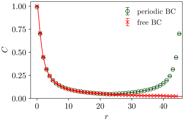
To generate the correlated bonds numerically we utilized the Fourier Filtering Method (FFM) Makse et al. (1996); Ahrens and Hartmann (2011). The FFM is a procedure to create stationary correlated random numbers of previously independent random numbers. Because it is based on the convolution theorem it is possible to benefit from the computationally efficient Fast Fourier Transform Algorithm Cooley and Tukey (1965). For its implementation we relied upon the functions of the FFTW library, version 3.3.5 Frigo and Johnson (2005). Figure 1 shows the average bond correlation along the main axes of a system with spins calculated by the estimator,
| (3) |
Here denotes the average with respect to the disorder. contains those bonds for which the bond is also on the lattice. The fact that does not contain all the bonds in is due to the free boundary conditions in one direction. The point is that for vectors which are not exactly parallel to the free boundary, the bond does not exist for all bonds of . For the correlations shown in Figure 1 we only investigated the directions parallel and perpendicular to the free boundary.
II.2 Ground States and Domain Walls
The nature of the ground state (GS) of the two-dimensional Ising spin glass is an intriguing subject on its own Newman and Stein (2000); Arguin and Damron (2014). Furthermore, GS computations of finite systems are a well established tool Hartmann and Rieger (2002, 2004) to investigate the glassy behavior of the model in the zero-temperature limit Hartmann (2008). The GS is the spin configuration which minimizes Eq. (1) for a given realization of the bonds. In case of two-dimensional planar lattices there exist exact procedures to generate the GS with a polynomial worst-case running time. This is in contrast to the three or higher-dimensional variants which belong to the class of NP-hard problems Barahona (1982).
There is more than one approach to compute the GS of two-dimensional planar spin glasses, such as the algorithm of Bieche et al. Bieche et al. (1980) and that of Barahona et al. Barahona et al. (1982). The key idea of these algorithms is to create a mapping from the original problem defined on the underlying lattice graph of the spin glass onto a related graph which is constructed in such a manner that the GS can be extracted from a minimum-weight perfect matching, which is polynomially computable. In this work we applied an ansatz which includes Kasteleyn-city subgraphs into the mapping process and thus is more efficient Pardella and Liers (2008); Thomas and Middleton (2007) in terms of speed and memory usage than the above mentioned algorithms. This allowed us to investigate systems up to a linear system size of spins in each direction without needing excessive computational resources. For the computation of the minimum-weight perfect matching the Blossom algorithm Cook and Rohe (1999) implemented by A. Rohe Rohe was utilized.
To study the spin glass at nonzero temperature we create domain wall (DW) excitations in the system. This was done by computing GSs under periodic and antiperiodic BCs also referred to as P-AP Carter et al. (2002). It works as follows. First, a spin glass with periodic BCs in one direction and free BCs in the other direction is generated with quenched disorder, . Then, its GS configuration, , is computed. Next, the periodic BCs are replaced by antiperiodic BCs by reversing the sign of one column of bonds parallel to the direction of periodicity, which leads to . Afterwards, the new GS configuration, , is calculated. The change of the BCs imposes a DW of minimal energy between the two spin configurations and . The energy of the DW is given by
| (4) |
The geometrical structure of a DW can be characterized by the number of bonds which are included in the surface. To avoid including those bonds which are a direct result of the different BCs, the surface is defined to consist of those bonds which fulfill , where runs over all unordered pairs of nearest neighbor lattice sites Khoshbakht and Weigel (2018).
III Results
We have obtained exact ground states for systems with correlation exponents in the range , where corresponds to independently sampled bonds. Since the GS calculation requires only polynomial time as a function of the system size, we were able to study sizes up to a large value of for each value of . For each value of and , we performed an average over many realizations of the disorder, ranging from realizations for the smallest sizes, 10000 realizations for , to 2000 realizations for the largest system size.
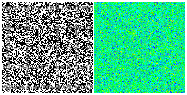
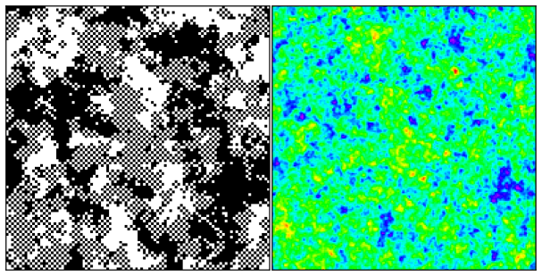
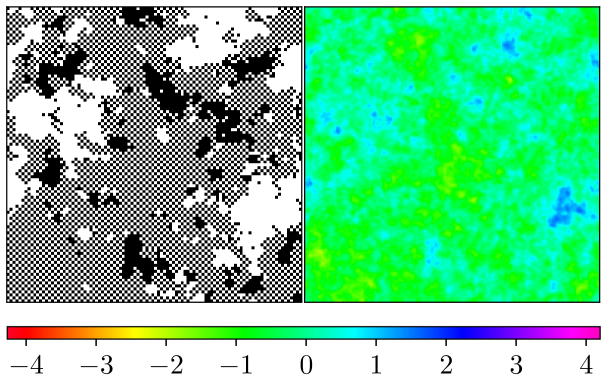
Figure 2 provides a first impression how the bond correlation impacts the ordering of the GS. It is apparent that for strong correlations there are large areas where the spins are either in ferromagnetic or antiferromagnetic order. This is related to there being large areas where, due to the correlation, the bonds have identical sign.
III.1 Domain Wall Energy
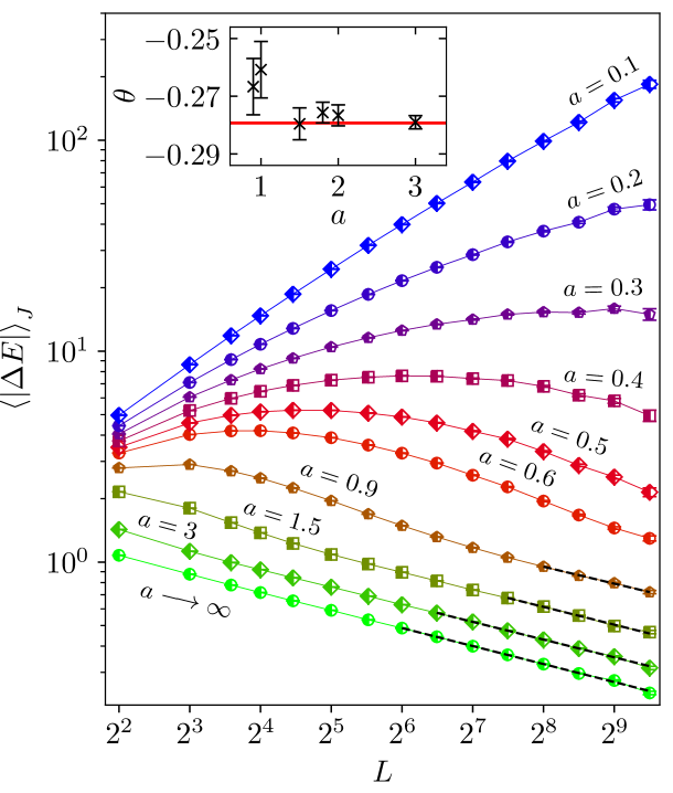
Next, we look at the influence of bond correlation on the properties of the previously discussed DW excitations. The absolute value of the DW energy is proportional to the coupling strength between block spins in the zero-temperature limit Bray and Moore (1987a). A stable order is possible if the average absolute value of the DW energy increases with the system size. In the uncorrelated case, , one obtains a power law behavior Bray and Moore (1987a); Hartmann and Young (2001); Hartmann et al. (2002); Khoshbakht and Weigel (2018),
| (5) |
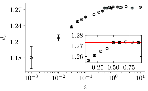
where is the stiffness exponent with its current best estimate Khoshbakht and Weigel (2018). Since there is no stable spin-glass phase for temperatures larger than zero. Figure 3 shows the impact of bond correlation on the scaling of . For one can still observe the pure power-law decay of the uncorrelated model on sufficiently long length scales. The inset demonstrates that, in this region, the stiffness exponent stays constant at a value equal to that of the uncorrelated model. For values of the average initially grows with system size, but starts to decrease for larger sizes, i.e. the curves exhibit a peak. The system size at the peak, , shifts to larger system sizes on decreasing the correlation exponent . This will be analyzed below.
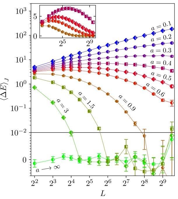
First we show in figure 4 the results for the average DW energy , which behaves in a somewhat similar manner as the average of the absolute value.
If spin-glass order existed in this model for some value of one would observe an increase in the limit , while at the same time would remain at, or converge to, zero as a function of . The latter indicates the absence of ferromagnetic order, but not necessarily the absence of spin glass order because for a spin glass the change of the boundary conditions from periodic to antiperiodic is symmetric, i.e., could either increase or decrease the GS energy, so the average would be zero even in the case of spin glass order. An increase of both and for small values of and corresponds to a ferro/antiferromagnetic ordering on local length scales, which is visible in Fig. 2 and will be discussed more below. Whether there is a true ordered phase for very small values of will be discussed next.
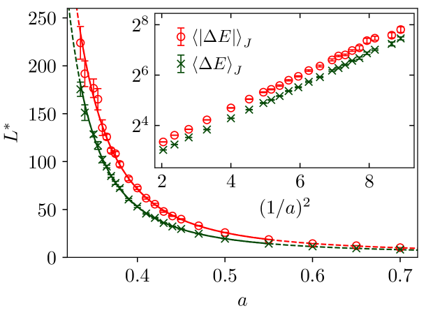
To track how the length scale of local order changes as a function of the correlation strength we measure the size at the peak, , for both the domain-wall energy and the absolute value, as a function of the correlation exponent . Numerically, was computed by fitting a parabola in the vicinity of the peaks of and . As the fit in figure 5 demonstrates, the data for is well described by an exponential function
| (6) |
A non-zero value of would indicate that an ordered phase exists for . A true spin-glass phase would be possible if for is smaller than for . We obtained values of for and for with quality of the fit and , respectively. Thus, a zero value for the critical correlation exponent parameter seems likely.
To consider this further, we set to zero and obtain the values of the other fit parameters, which here are , , () for and , , () for . Since the qualities of the fits remain almost identical in comparison to the data is considered to be consistent with , which would imply that there is no global order when , either ferromagnetic or spin glass. The inset shows that the behavior of is also compatible with . Fits of this type, with and fixed, have quality of the fit larger than , which is reasonable. Note that an exponential dependence of the “breakup” length scale of ferromagnetic order as a function of disorder strength was also found in the two-dimensional random field Ising model, both at low temperatures Pytte and Fernandez (1985) and in the GS Seppälä et al. (1998).
III.2 Domain Wall Surface
The behavior of DW surfaces is regarded as one of the essential parameters which describe the properties of random systems Bray and Moore (1987b); Newman and Stein (2007). DWs separate spins in GS and reversed GS. Their surface is defined as those bonds which belong to the DW, and we denote the surface size by .
In the uncorrelated case, , the average DW surface size exhibits a power law Kawashima (2000); Melchert and Hartmann (2007),
| (7) |
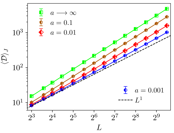
where is the fractal surface dimension, for which the best numerical estimate at present is Khoshbakht and Weigel (2018). When the system is a ferro/antiferromagnet and , implying that , i.e., the surface is not fractal here. Figure 6 shows the scaling of the DW surface size for different values of . In general, it can be seen that the correlation decreases the number of bonds in the DW surface. Even for , the data on this log-log plot shows a visible a visible deviation from the linear behavior which occurs for strictly zero.
To characterize this behavior we fitted pure power-laws to the data. For this purpose, we did not do a full fit to all data points, but used the sliding-window approach instead. Here, four values of which are adjacent in terms of system size were grouped together in one fit window, respectively. The independent variables of such a fit window were given by with , . The dependent variables corresponded to the data, i.e. . The smallest independent variable of each fit window is denoted as .
For each window, we fitted the power law to the data resulting in a value of . The dependence of as a function of for different values of can be found in figure 7. In the uncorrelated case decreases as a function of , whereas for strong correlations increases. In any case, for system sizes and small values we observed some notable dependence of on the system size. This motivated us to include corrections to scaling the power law behavior in Eq. (7) by considering Khoshbakht and Weigel (2018); Hartmann and Moore (2003)
| (8) |
By using Eq. (8) the quality of the fit is larger than for all studied values of with smallest linear system size of the fit . For larger values of , the pure linear fit was always fine, given our statistical accuracy. Figure 8 shows the resulting fractal surface dimension for all considered values of . At the fractal surface dimension starts to decline from Khoshbakht and Weigel (2018), in the uncorrelated case, to smaller values. This is also visible in Fig. 7. Thus, it appears that for small values of the fractal structure of the cluster changes, although there is no phase transition. Note that, in order to extract , we also performed fits of the form (not shown; and also depend on ) to the sliding window fractal dimensions shown in Fig. 7. The behavior of this extrapolated fractal dimension also exhibits the same notable decrease of for . Of course, it can not be ruled out that on sufficiently large length scales, i.e., for much larger sizes than are currently accessible, the fractal dimension of the uncorrelated model would be recovered again and thus Khoshbakht and Weigel (2018) for all values .
III.3 Spin Correlations in the Ground State
In this section the effects of the bond correlations on spin correlations in the GS will be discussed. Note that at zero temperature there is no thermal disorder and, in our study which uses bonds with a continuous distribution, the ground state is non-degenerate apart from overall spin inversion.
The two-point spin correlation is given by , where denotes a spin in the GS configuration. In the uncorrelated model if . The correlated bonds induce a local ferro/antiferromagnetic order into the GS. When the system is a ferro/antiferromagnet and the order is global. In the ferromagnetic case and in the antiferromagnetic case alternates between plus and minus one. Therefore, the GS spin correlation can be estimated by
| (9) | ||||
and . , similar to Eq. (3), contains those sites for which is on the lattice, given the free BC in one direction. Note that this definition means that the correlation is measured for each site on one of the two sublattices of a checkerboard partition of the square lattice, such that the correlation is insensitive to whether the order is ferromagnetic or antiferromagnetic.
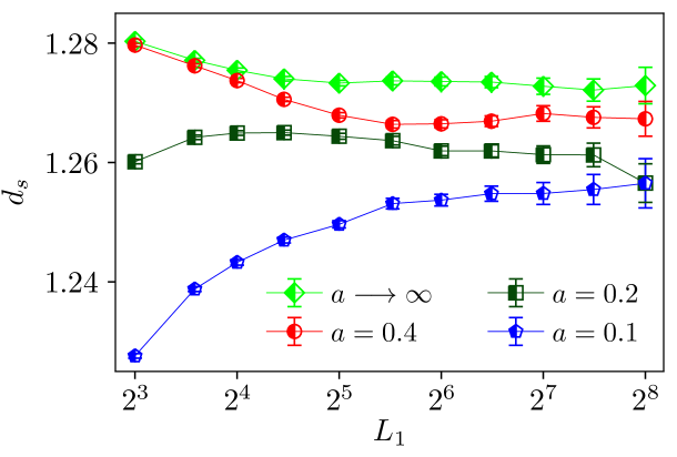
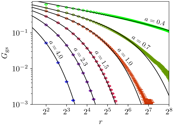
In figure 9 one can see the GS correlation for different values of . The data is well described by a scaling form of type
| (10) |
From the perspective of ordering we are especially interested in the correlation length, , that provides the distance over which spins are notably correlated. The straightforward method to extract is by fitting the function of Eq. (10) to the data. The problem with such an approach is that neither nor are known. Also finite-size corrections reduce the match between scaling form and actual data. Thus, we used different approaches to obtain .
First, we perform a separate fit for each value of down to small correlations where the error bars start to exceed one quarter of the correlation value. We observed that for , the values of the exponents and did not change much, while for smaller values of the exponents were a bit smaller. Therefore, we fixed the exponents to the (averaged) values seen for and fitted only with respect to .
Second, we also performed a multifit, i.e., we fitted the correlation function simultaneously Hartmann (2015) with one value for , one value for and values of the correlation length at many values of . The results of this multifit are also shown in Fig. 9. The obtained values for for these two fitting approaches are shown in Fig. 10. As can be seen, the results from fixing the values of the exponents and from using the multifit approach do not differ much.
Before we discuss the behavior of , we describe the third approach we have used to estimate the correlation length. Here, we used the integral estimator that was introduced in Ref. Belletti et al. (2008). It presupposes that for the correlation function is dominated by a power law of type , whereas for the correlation is negligible. As a consequence, the integral
| (11) |
is given by and thus
| (12) |
This result would be exact and independent of if the correlation actually was only a power law. For real correlations, the value of dictates which part of the correlation function contributes most to the integral. Because such a scaling approach is only valid when is much larger than the lattice constant a high value of reduces the systematic error of the method. On the other hand, large values of increase the statistical error of . Following the recommendation of Belletti et al. (2009) we used as a compromise. Note that since the statistical error of the measured correlation grows with distance , one usually defines a cutoff distance up to which the data is directly used for the integral. Similar to Belletti et al. (2009) we specified this cutoff distance as the value of where is smaller than three times its error. For values of larger than this cutoff distance we computed the integral up to the maximal length of from fits to Eq. (10). The start value of these fits were set to . Because it was observed that the correlation decays slightly differently along the directions with free and periodic BCs, the computations of the GS were also done with an independent set of simulations for full free BCs.
Next, the correlation length was extracted from the average of the GS correlation, , along the main axes. The statistical error of was estimated by bootstrapping Young (2015); Hartmann (2015) and the integrals according to Eq. (11) were computed by utilizing the midpoint integration rule. For small values of , the contribution to from the integral beyond the cutoff gets increasingly large. For instance, when this contribution made up approximately of the value of . Hence, to estimate the total error, we added an extra systematic error to the statistical error. This was done by analyzing the value of for two other choices of the cutoff distance, i.e., being the distance where the error of the correlation function is two or four times larger than its estimate, respectively. The maximal deviation of these two values from the standard definition, which uses a magnitude of three error bars to define cutoff, was set to be the systematic error. Furthermore, because the statistical error of grows large for small values of the correlation exponent and the system has to be sufficiently large to neglect boundary effects, values of were not considered for this approach.
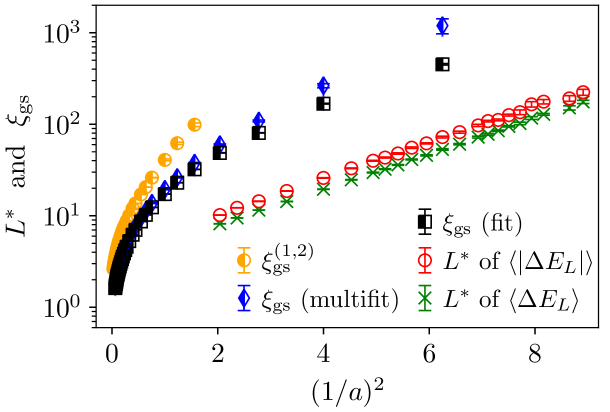
Figure 10 shows as a function of the correlation exponent. In contrast to the data for the length scales , the plot shows that the behavior of none of the three correlation lengths that we have defined, and , is close to exponential. Nonetheless, for the correlation lengths may converge to this behavior. We found that the data for these three definitions of the correlation length could be well fit to a function of the type
| (13) |
The exponential in Eq. (13) is consistent with the previous results for the length scale and will dominate for . The power-law part is chosen to describe the behavior for large values of .
We have fitted the data to this function. For example, for the data obtained from the multifit we again obtained a small value of . Thus once again we fixed in order to determine the values of the remaining fit parameters, obtaining , , and with a good quality of the fit. Similar values, in particular for , are found for the other two definitions of that we used. This means that for large values of the correlation exponent the behavior of the correlation length as function of seems to be better described by a power law. Also, the behavior of the peak lengths and of the ferromagnetic correlation lengths differ a lot, but it is still possible that for very small values of , an exponential dependence of on would be recovered. Unfortunately, to investigate this issue much larger system sizes would have to be treated, well beyond current numerical capabilities.
IV Discussion
The standard two-dimensional Ising spins glass does not exhibit a finite-temperature spin glass phase in contrast to the three or higher dimensional cases Young and Stinchcombe (1976); Southern and Young (1977); Hartmann and Young (2001). This work deals with the question how long-range correlated bonds influence this characteristic. Therefore, the ordering behaviour of the two-dimensional Ising spin glass with spatially long-range correlated bonds is studied in the zero-temperature limit. The bonds are drawn from a standard normal distribution with a two-point correlation for bond distance that decays as , . In the borderline case, when , the system is either a ferromagnet or antiferromagnet, depending on the bond realization. For the uncorrelated EA model is recovered.
For we observed that the correlation has local effects on the zero-temperature ordering behaviour. The correlation locally effects the average value of the bonds as well as their standard deviation for each individual realization of the disorder. These parameters are decisive to distinguish between a spin glass or ferro/antiferromagnet in case of the uncorrelated model Sherrington and Southern (1975); Monthus and Garel (2014). In correspondence to that, the spin correlation of the GS reveals how the correlation induces a local ferro/antiferromagnetic order into the GS. This is reflected by a growing correlation length when decreasing .
Complementary results to the direct study of the GS spin configurations were obtained by investigating DW excitations. The average of the absolute value of the DW energy can be interpreted as the coupling strength between block spins at zero temperature Bray and Moore (1987a). We found, that for strong bond correlation, the average of absolute value of the DW energy initially increases as a function of the system size up to a peak, and then decreases. Since we made the same observation for the actual DW energy it shows that the increase of the absolute value of the DW energy is a consequence of local ferro/antiferromagnetic order of the system in GS. The system size where the peak occurs, , is interpreted as the length scale of local order. For small values of the correlation exponent , both and the correlation length of the GS, , can be described by an exponential divergence. Interestingly, a similar exponential length scale was also found in the two-dimensional random field Ising model by GS computations Seppälä et al. (1998) and at low temperatures Pytte and Fernandez (1985). In these studies the length scale of ferromagnetic order was examined as a function of the standard deviation of the random magnetic field.
For the two-dimensional Ising spin glass, the distribution of the absolute value of the domain wall energy is “universal” with respect to the initial bond distribution. This means for any continuous, symmetric bond distribution with sufficiently small mean and finite higher moments, the absolute value of the domain wall energy should approach the same scaling function McMillan (1984); Bray and Moore (1987a); Amoruso et al. (2003). Thus, we expect the same kind of universality for our model.
The stiffness exponent describes the scaling of the width of this distribution, and is related to the critical exponent describing the divergence of the correlation length as by Fernandez et al. (2016); Bray and Moore (1987a). At this zero temperature transition is the only independent exponent. Therefore, any bond correlation which leaves the stiffness exponent unchanged does not influence the universality of the model. From the data of it is expected that there is no global ordered phase for . This implies that the stiffness exponent is negative for . Furthermore, for values of in the range the stiffness exponent stays equal to the uncorrelated case. Due to the limited range of studied length scales it was not possible for us to verify this for values of less than .
In addition to the DW energy, another important parameter to describe the low-temperature behaviour of the Ising spin glass is the DW surface area Bray and Moore (1987b); Newman and Stein (2007). In the uncorrelated model the domain-wall surface area follows a power law, , where Khoshbakht and Weigel (2018). Our results are compatible to this for all considered correlation exponents . At the fractal surface dimension starts to decline. For the values of the data is well described by a power law with scaling corrections Hartmann and Moore (2003); Khoshbakht and Weigel (2018), i.e. . The decrease in implies that for strong correlations DWs with shorter lengths are energetic favorable. In the extreme case when the system is a ferro/antiferromagnet and thus . Of course, it can not be ruled out that the decline in is local and on sufficiently long length scales the pure power law with Khoshbakht and Weigel (2018) is recovered again for all .
In this context it is interesting to note that there exists a proposed relation which links the stiffness exponent with the fractal surface dimension, namely Amoruso et al. (2006). According to highly accurate numerical results Khoshbakht and Weigel (2018) this equation is probably not exact. Our results for the fractal surface dimension () and the stiffness exponent () deviate by approximately 6.5 standard deviations from the mentioned conjecture, since . The latter result was obtained by using standard error propagation, thus, neglecting correlations between the estimates of and which exist because both values were obtained from the same data set. Nonetheless, our results also support the conclusion that the proposed scaling relation is not exact.
In conclusion, it is observed that correlation among the bonds has strong effect on the ordering on local length scales, inducing ferro/antiferromagnetic domains into the GS. The length scale of local ferro/antiferromagnetic order diverges exponentially when the correlation exponent approaches zero. The fractal surface dimension decreases for strong correlations on the studied length scales. No signature of a spin-glass phase at finite temperature is observed.
Acknowledgements.
The simulations were performed at the HPC cluster CARL, located at the University of Oldenburg (Germany) and funded by the DFG through its Major Research Instrumentation Programme (INST 184/157-1 FUGG) and the Ministry of Science and Culture (MWK) of the Lower Saxony State.References
- Vincent and Dupuis (2018) E. Vincent and V. Dupuis, in Frustrated Materials and Ferroic Glasses, edited by T. Lookman and X. Ren (Springer, Cham, 2018) pp. 31–56.
- Edwards and Anderson (1975) S. F. Edwards and P. W. Anderson, J. Phys. F 5, 965 (1975).
- Sherrington and Kirkpatrick (1975) D. Sherrington and S. Kirkpatrick, Phys. Rev. Lett. 35, 1792 (1975).
- Stein and Newman (2013) D. L. Stein and C. M. Newman, Spin Glasses and Complexity (Princeton University Press, Princeton, 2013).
- Mézard et al. (1987) M. Mézard, G. Parisi, and M. Virasoro, Spin Glass Theory and Beyond (World Scientific, Singapore, 1987).
- Young (1998) A. P. Young, ed., Spin Glasses and Random Fields (World Scientific, Singapore, 1998).
- Bolthausen and Bovier (2007) E. Bolthausen and A. Bovier, eds., Spin Glasses (Springer, Berlin, Heidelberg, 2007).
- Nishimori (2001) H. Nishimori, Statistical Physics of Spin Glasses and Information Processing: An Introduction (Oxford University Press, Oxford, 2001).
- Dotsenko (1994) V. Dotsenko, An introduction to the theory of spin glasses and neural networks (World Scientific, Singapore, 1994).
- Hartmann and Rieger (2002) A. K. Hartmann and H. Rieger, Optimization Algorithms in Physics (Wiley-VCH, Weinheim, 2002).
- Hartmann and Rieger (2004) A. K. Hartmann and H. Rieger, eds., New Optimization Algorithms in Physics (Wiley-VCH, Weinheim, 2004).
- Zhu et al. (2015) Z. Zhu, A. J. Ochoa, and H. G. Katzgraber, Phys. Rev. Lett. 115, 077201 (2015).
- McMillan (1984) W. L. McMillan, J. Phys. C 17, 3179 (1984).
- Bray and Moore (1987a) A. J. Bray and M. A. Moore, in Heidelberg Colloquium on Glassy Dynamics, edited by J. van Hemmen and I. Morgenstern (Springer, Berlin, Heidelberg, 1987) pp. 121–153.
- Fisher and Huse (1988) D. S. Fisher and D. A. Huse, Phys. Rev. B 38, 386 (1988).
- Hartmann and Moore (2003) A. K. Hartmann and M. A. Moore, Phys. Rev. Lett. 90, 127201 (2003).
- Hartmann and Moore (2004) A. K. Hartmann and M. A. Moore, Phys. Rev. B 69, 104409 (2004).
- Young and Stinchcombe (1976) A. P. Young and R. B. Stinchcombe, J. Phys. C 9, 4419 (1976).
- Southern and Young (1977) B. W. Southern and A. P. Young, J. Phys. C 10, 2179 (1977).
- Hartmann and Young (2001) A. K. Hartmann and A. P. Young, Phys. Rev. B 64, 180404(R) (2001).
- Khoshbakht and Weigel (2018) H. Khoshbakht and M. Weigel, Phys. Rev. B 97, 064410 (2018).
- Parisen Toldin et al. (2011) F. Parisen Toldin, A. Pelissetto, and E. Vicari, Phys. Rev. E 84, 051116 (2011).
- Thomas et al. (2011) C. K. Thomas, D. A. Huse, and A. A. Middleton, Phys. Rev. Lett. 107, 047203 (2011).
- Fernandez et al. (2016) L. A. Fernandez, E. Marinari, V. Martin-Mayor, G. Parisi, and J. J. Ruiz-Lorenzo, Phys. Rev. B 94, 024402 (2016).
- Sherrington and Southern (1975) D. Sherrington and W. Southern, J. Phys. F 5, L49 (1975).
- Amoruso and Hartmann (2004) C. Amoruso and A. K. Hartmann, Phys. Rev. B 70, 134425 (2004).
- Fisch and Hartmann (2007) R. Fisch and A. K. Hartmann, Phys. Rev. B 75, 174415 (2007).
- Monthus and Garel (2014) C. Monthus and T. Garel, Phys. Rev. B 89, 184408 (2014).
- Fajen et al. (2020) H. Fajen, A. K. Hartmann, and A. P. Young, Phys. Rev. E 102, 012131 (2020).
- Weinrib and Halperin (1983) A. Weinrib and B. I. Halperin, Phys. Rev. B 27, 413 (1983).
- Ahrens and Hartmann (2011) B. Ahrens and A. K. Hartmann, Phys. Rev. B 84, 144202 (2011).
- Nattermann (1998) T. Nattermann, in Spin Glasses and Random Fields, edited by A. P. Young (World Scientific, Singapore, 1998) pp. 277–298.
- Makse et al. (1996) H. A. Makse, S. Havlin, M. Schwartz, and H. E. Stanley, Phys. Rev. E 53, 5445 (1996).
- Cooley and Tukey (1965) J. W. Cooley and J. W. Tukey, Mathematics of Computation 19, 297 (1965).
- Frigo and Johnson (2005) M. Frigo and S. G. Johnson, Proceedings of the IEEE 93, 216 (2005).
- Newman and Stein (2000) C. M. Newman and D. L. Stein, Phys. Rev. Lett. 84, 3966 (2000).
- Arguin and Damron (2014) L.-P. Arguin and M. Damron, Annales de l’I.H.P. Probabilités et statistiques 50, 28 (2014).
- Hartmann (2008) A. K. Hartmann, in Rugged Free Energy Landscapes, edited by W. Janke (Springer, Berlin, Heidelberg, 2008) pp. 67–106.
- Barahona (1982) F. Barahona, J. Phys. A 15, 3241 (1982).
- Bieche et al. (1980) L. Bieche, J. P. Uhry, R. Maynard, and R. Rammal, J. Phys. A 13, 2553 (1980).
- Barahona et al. (1982) F. Barahona, R. Maynard, R. Rammal, and J. Uhry, J. Phys. A 15, 673 (1982).
- Pardella and Liers (2008) G. Pardella and F. Liers, Phys. Rev. E 78, 056705 (2008).
- Thomas and Middleton (2007) C. K. Thomas and A. A. Middleton, Phys. Rev. B 76, 220406(R) (2007).
- Cook and Rohe (1999) W. Cook and A. Rohe, INFORMS Journal on Computing 11, 138 (1999).
- (45) A. Rohe, “The Blossom Four Code for Min-Weight Perfect Matching,” https://www.math.uwaterloo.ca/ bico/blossom4/.
- Carter et al. (2002) A. C. Carter, A. J. Bray, and M. A. Moore, Phys. Rev. Lett. 88, 077201 (2002).
- Hartmann et al. (2002) A. K. Hartmann, A. J. Bray, A. C. Carter, M. A. Moore, and A. P. Young, Phys. Rev. B 66, 224401 (2002).
- Pytte and Fernandez (1985) E. Pytte and J. F. Fernandez, J. Appl. Phys. 57, 3274 (1985).
- Seppälä et al. (1998) E. T. Seppälä, V. Petäjä, and M. J. Alava, Phys. Rev. E 58, R5217 (1998).
- Bray and Moore (1987b) A. J. Bray and M. A. Moore, Phys. Rev. Lett. 58, 57 (1987b).
- Newman and Stein (2007) C. M. Newman and D. L. Stein, in Spin glasses, edited by E. Bolthausen and A. Bovier (Springer, Berlin, Heidelberg, 2007) pp. 145–158.
- Kawashima (2000) N. Kawashima, J. Phys. Soc. Jpn. 69, 987 (2000).
- Melchert and Hartmann (2007) O. Melchert and A. K. Hartmann, Phys. Rev. B 76, 174411 (2007).
- Hartmann (2015) A. K. Hartmann, Big Practical Guide to Computer Simulations (World Scientific, Singapore, 2015).
- Belletti et al. (2008) F. Belletti, M. Cotallo, A. Cruz, L. A. Fernandez, A. Gordillo-Guerrero, M. Guidetti, A. Maiorano, F. Mantovani, E. Marinari, V. Martin-Mayor, A. M. Sudupe, D. Navarro, G. Parisi, S. Perez-Gaviro, J. J. Ruiz-Lorenzo, S. F. Schifano, D. Sciretti, A. Tarancon, R. Tripiccione, J. L. Velasco, and D. Yllanes, Phys. Rev. Lett. 101, 157201 (2008).
- Belletti et al. (2009) F. Belletti, A. Cruz, L. A. Fernandez, A. Gordillo-Guerrero, M. Guidetti, A. Maiorano, F. Mantovani, E. Marinari, V. Martin-Mayor, J. Monforte, et al., J. Stat. Phys. 135, 1121 (2009).
- Young (2015) A. P. Young, Everything You Wanted to Know About Data Analysis and Fitting but Were Afraid to Ask (Springer, Cham, 2015).
- Amoruso et al. (2003) C. Amoruso, E. Marinari, O. C. Martin, and A. Pagnani, Phys. Rev. Lett. 91, 087201 (2003).
- Amoruso et al. (2006) C. Amoruso, A. K. Hartmann, M. B. Hastings, and M. A. Moore, Phys. Rev. Lett. 97, 267202 (2006).