Ordinal Synchronization: Using ordinal patterns to capture interdependencies between time series
Abstract
We introduce Ordinal Synchronization () as a new measure to quantify synchronization between dynamical systems. is calculated from the extraction of the ordinal patterns related to two time series, their transformation into -dimensional ordinal vectors and the adequate quantification of their alignment. provides a fast and robust-to noise tool to assess synchronization without any implicit assumption about the distribution of data sets nor their dynamical properties, capturing in-phase and anti-phase synchronization. Furthermore, varying the length of the ordinal vectors required to compute it is possible to detect synchronization at different time scales. We test the performance of with data sets coming from unidirectionally coupled electronic Lorenz oscillators and brain imaging datasets obtained from magnetoencephalographic recordings, comparing the performance of with other classical metrics that quantify synchronization between dynamical systems.
keywords:
Synchronization , ordinal patterns , in-phase synchronization , anti-phase synchronization , nonlinear electronic circuits , brain imaging data sets.Since the seminal work of Huygens about the coordinated motion of two pendulum clocks (refereed to as “an odd kind of sympathy”) [1], the study of synchronization in real systems has been one of the major research lines in nonlinear dynamics. From fireflies to neurons, synchronization has been reported in a diversity of social (e.g., human movement or clapping) [2, 3], biological (e.g., brain regions or cardiac tissue) [4, 5] and technological systems (e.g., wireless communications or power grids) [6, 7], being in many cases a fundamental process for the functioning of the underlying system. However, despite being an ubiquitous phenomenon, the detection and quantification of synchronization can be a difficult task. The main reasons are the diversity of kinds of synchronization [8], the complexity of interaction between dynamical systems [9], the existence of unavoidable external perturbations [10] or the inability of observing all variables of a real system [11], just to name a few.
As a consequence, there is not a unique way of quantifying the amount of synchronization in real time series and a series of metrics have been proposed with this purpose. As a rough approximation, these metrics can be classified into three main groups: (i) linear, (ii) nonlinear and (iii) spectral metrics. While linear metrics, such as the Pearson correlation coefficient, are the most straightforward to be calculated and less time consuming, they suppose the existence of a linear correlation between time series, an assumption that is not fulfilled in the majority of real cases. On the other hand, nonlinear metrics asume a certain nonlinear coupling function between a variable and a variable , such as . However the estimation of the nonlinear function renders impossible in the majority of cases and certain assumptions have to be assumed for quantifying synchronization. Measures such as the mutual information or the phase locking value are examples of nonlinear metrics, the former assuming a certain statistical interdependency between signals and the latter considering only a phase relation. Finally, spectral metrics, such as the coherence or the imaginary part of coherence, translate the problem to the spectral domain, analyzing the relation between the spectra obtained from the original time series assuming linear/nonlinear relations (see [12] for a thorough review about metrics quantifying synchronization in real data sets).
In the current paper we are concerned about using ordinal patterns, a symbolic representation of temporal data sets, to define a new metric that is able to reveal the synchronization between time series. Bahraminasab et. al. [13] used a symbolic dynamics approach to design a directionality index parameter. Transforming the increment between successive points within a times series into ordinal patterns, authors calculated the mutual information between a process at time and a process at time and next obtained the directionality index as defined in [14]. Applying this methodology to respiratory and cardiac recordings it is possible to quantify how respiratory oscillations have more influence on cardiac dynamics than vice-versa [13]. More recently, Li et al. used a similar indicator to evaluate the directionality of the coupling in time series consisting of spikes [15]. Using the Izhikevich neuron model [16], authors showed how that methodology was robust for weak coupling strengths, in the presence of noise or even with multiple pathways of coupling between neurons. More recently, Rosário et. al. [17] used the ordinal patterns observed in EEG datasets, also known as “motifs” [18], to construct time varying networks and analysed their evolution along time and the properties of the averaged functional network. Specifically, the amount of synchronization between a pair of recorded electrodes of an EEG was obtained by evaluating the number of ordinal patterns co-ocurring at the same time but also at a given lag time steps. Using both positive and negative values of authors were able to quantify the direction of the interaction between the two time series, i.e., the causality, to further construct temporal time networks. Next, they showed how the resulting time varying functional networks were able to identify those brain regions related to information processing and found differences between healthy individuals and patients suffering from chronic pain [17].
In this paper, we also propose the use of symbolic dynamics to evaluate the level of synchronization between time series. However, our methodology consists in a measure of synchronization that does not take into account the existence of a delay time between time series, despite further adaptation to this case is also possible (see Section Conclusions). As in the case of [13, 18, 17], we take advantage of the transformation of a time series into a concatenated series of -dimensional ordinal patterns [19] that allow us to quantify the amount of synchronization between two (or more) symbols sequences. The main advantage of our methodology is that it takes into account both the in-phase and anti-phase synchronization of two dynamical systems, the latter being disregarded in the aforementioned proposals based on ordinal patterns.
We have calculated the of two kind of data sets: (i) unidirectionally coupled Lorenz electronic systems and (ii) magnetoencephalographic (MEG) recordings measuring the activity of sensors placed at the scalp of an individual during resting state. Next, we compared the amount of synchronization computed by OS with respect to those obtained from classical metrics like phase locking value (PLV), mutual information (MI), spectral coherence (SC) and Pearson correlation (r).
1 Materials and Methods
1.1 Defining Ordinal Synchronization
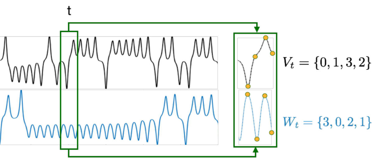
To compute the (OS) between two time series and , we first extract their -dimensional ordinal patterns [19]. In this way, we choose a length D and divide both time series of length M into equal segments. Next, we obtain the order of the values included inside each segment, also called the ordinal patterns: l
| (1) | ||||
| (2) |
where and are the ordinal vectors inside the segment given by , elements refer to the ordinal position of the values in and , respectively. Note that the elements in and are natural numbers ranging from to . The higher the value in the time series, the higher the corresponding element in the ordinal vector. Following the example depicted in Fig. 1, where , we obtain:
| (3) | ||||
| (4) |
Then, we take the euclidean norm of each ordinal vector.
| (5) |
and we call and the normalized vectors. Note that this step only depends on the length D.
Now, we define the raw value of the instantaneous ordinal synchronization at time () as the dot product between both ordinal ordinal vectors (i.e., ). For a more intuitive interpretation, we linearly rescale the value of to be bounded between and :
| (6) |
where is the minimum possible value of the scalar product between two ordinal vectors. Note that, since the elements of the ordinal vectors are always positive and have only one component equal to zero, the lowest possible scalar product between and is obtained when the order of the elements of vector is inverted in . In our example:
| (7) |
In general, for any vector of length D:
| (8) |
Following the normalization in 6), we ensure that two ordinal vectors that follow opposite evolutions will unambiguously lead to a value of , and two vectors whose elements have the same order will have an . Being the total number of ordinal vectors in time series of points, the final value of the ordinal synchronization for a given pair of time series and is obtained averaging the instantaneous values of along the whole time series:
| (9) |
Since we consider the of consecutive (i.e., non-overlapping) time windows, the value of in Eq. 9 is given by the expression , with being a natural number bounded by . Note that it is also possible to define a sliding just by increasing in one unit for every instead of considering consecutive windows.
1.2 Experimental results: Electronic Lorenz Systems
We analyzed the transition to the synchronized regime of two coupled Lorenz oscillators [20]. We implemented an electronic version of the Lorenz system, whose equations are detailed in Appendix B. Two Lorenz circuits are coupled unidirectionally in a master-slave configuration (see Fig. 2) with a coupling strength that can be modified. Our experiments include two conditions: in the first one, is modified in the absence of external noise; in the second one, varies in presence of Gaussian noise with band selection. The (AI0-AI3) input ports of a data acquisition (DAQ) card are used for sampling the and variables of each circuit, while the output ports AO0 and AO1 generate two different noise signals (, ) that perturb the dynamics of the Lorenz circuits through variable of each circuit. In this way, an external source of noise can be introduced to check the robustness of the experiments. The circuit responsible of the coupling strength is controlled by a digital potentiometer XDCP, which is adjusted by digital pulses from ports P00 and P01. Noisy signals were designed in LabVIEW, using a Gaussian White Noise library [21] that generates two different Gaussian-distributed pseudorandom sequences bounded between [-1 1]. All the experimental process is controlled by a virtual interface in LabVIEW 2016 (PC).
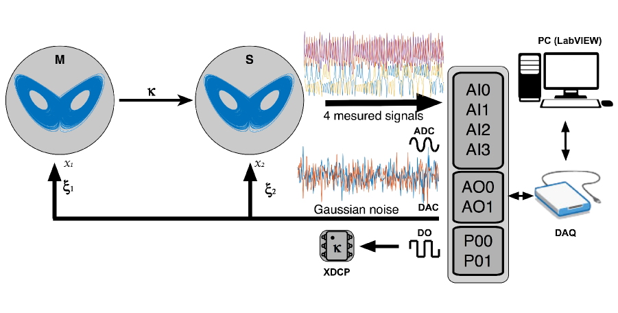
The experiment works in the following way: First, is set to zero and digital pulses (P00 and P01) are sent to the digital potentiometer until the highest value of is reached. Second, variables and of the circuits are acquired by the analog ports (AI0-AI3) in order to compute the synchronization metrics. Initially, we have obtained all results for , i.e., in the absence of external noise, and then, after a moderate amount of noise is introduced, all synchronization metrics are calculated again (See Appendix C). Every signal, with or without noise, has a length of 30000 samples.
1.3 Applications to magnetoencephalographic recordings
We have checked the performance of the in the context of neuroscientific datasets. Specifically, we quantified the level of synchronization between pairs of channels of MEG recordings. Data sets have been obtained from the Human Connectome Project (for details, see [22] and https://www.humanconnectome.org). The experimental data sets consist of MEG recordings of an individual during resting state for a period of approximately minutes each. During the scan, the subject were supine and maintained fixation on a projected red crosshair on a dark background. Brain activity was scanned with 241 magnetometers on a whole head MAGNES (4D Neuroimaging, San Diego, CA, USA) system housed in a magnetically shielded room. The root-mean-squared noise of the magnetometers is about fT/sqrt () on average in the white-noise range (above 2 ). Data was recorded at sampling rate of . Five current coils attached to the subject, in combination with structural-imaging data and head-surface tracings, were used to localize the brain in geometric relation to the magnetometers and to monitor and partially correct for head movement during the MEG acquisition. Artifacts, bad channels, and bad segments were identified and removed from the MEG recordings, which were processed with a pipeline based on independent component analysis to identify and clean environmental and subject’s artifacts [22].
2 Results
2.1 Nonlinear electronic circuits
In order to assess the validity of , we have explored its performance for different values of , from 3 to the full length of the time series under evaluation. Since it is the first time is used, we have compared it to classical measures of correlation, namely Pearson correlation coefficient (), spectral coherence (), phase locking value () and mutual information (). We have used two kinds of data sets to validate , on the one hand, experimental time series from nonlinear electronic circuits, and on the other hand, MEG recordings.
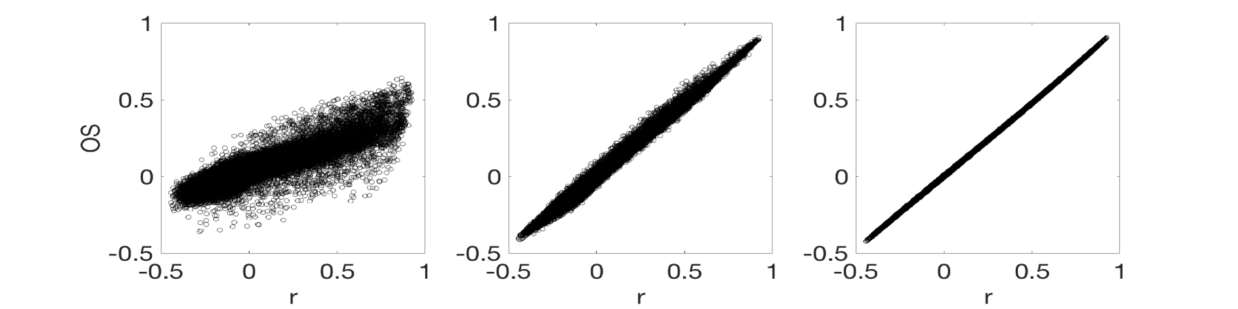
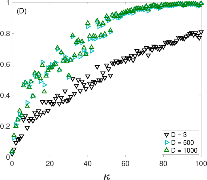
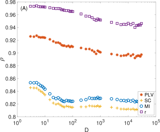
First, we take advantage of the ability of controlling the coupling strength between electronic circuits and investigate how changes as two dynamical systems smoothly vary their level of synchronization from being unsynchronized to completely synchronized. Specifically, two electronic Lorenz systems are unidirectionally coupled with a parameter controlling their coupling strength (see Appendix B for details). Initially, we do not perturb the oscillators with external noise (see Appendix C for the case of including external noisy signals). However, we can not avoid the intrinsic noise of the electronic circuits together with the tolerance of the electronic components (between 5 % and 10 %). Figure 3 shows how the value of changes as the coupling strength is increased from zero. Since the value of depends on the length of the ordinal vectors, we show the results for three different values: (Fig. 3A), (Fig. 3B) and (Fig. 3C). Note that, by increasing the length of the vectors, we are obtaining the amount of synchronization at different time scales. Together with , we plot the values of the rest of synchronization metrics in (A), (B) and (C), which remain unaltered in the three plots (since they do not depend on ).
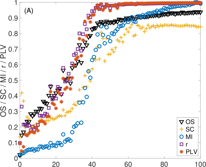
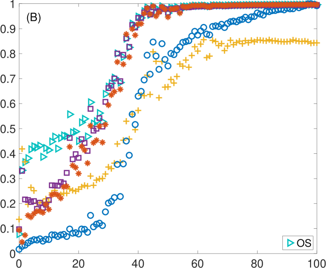
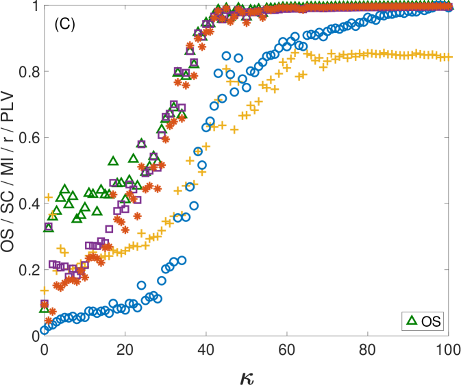
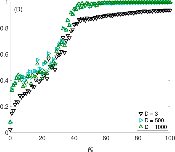
In all cases, we observe that increases for low to moderate values of and remains at a high value once a certain threshold is reached. This behaviour is similar to the rest of the synchronization metrics. However, both and seem to saturate at values of higher than , and , which seem to reach a plateau around . Figure 3D shows the comparison of for the three different values of . Here, we can also observe how at , has a different qualitative behaviour from and , since it stays around 0.9 and does not reach 1 as in the windows of longer lengths. The reason is the existence of intrinsic noise of the electronic circuits, that affects much more the alignment of the ordinal vectors of shorter lengths than those with higher dimensions.
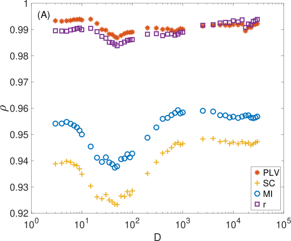
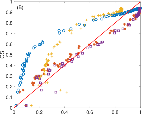
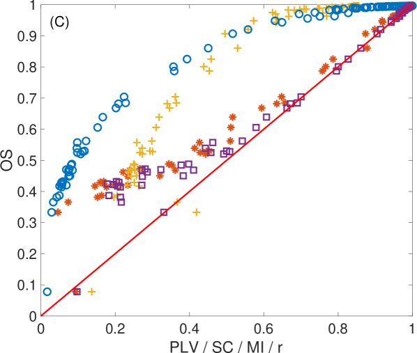
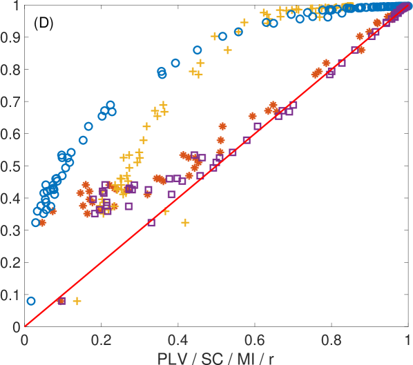
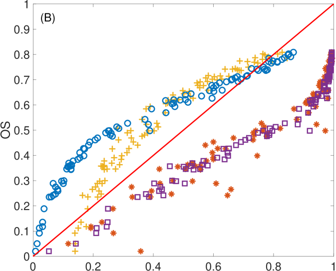
Figure 4 shows the average correlation () between each D-dependent and the rest of synchronization metrics with zero noise. Note that correlations are higher than in all cases, although it seems to be certain vector lengths that maximize these correlations. Also note that correlations with and are the highest and, in all cases, very close to 1. At the same time, and show lower correlations that, in turn, seem to be more dependent on the value of the vector length (see Fig. 4A).
We can investigate how is related to the rest of the synchronization metrics in more detail by setting the length of the ordinal vectors to a given value (, or in this case) and observe the influence of the level of synchronization (Fig. 4B, C and D). For any of the three selected lengths, shows a linear relation with and , especially at values of higher than . However, the relation with and seems to be nonlinear in all cases. Interestingly, for low levels of synchronization, increases much faster than these two latter metrics. While saturates around , finally increases faster than only for high values of synchronization, eventually reaching the value of around 1. Also note how, in the case of (Fig. 4B), the intrinsic noise of the electronic circuits prevents to reach the value of one. This behaviour can be observed even clearer in the case of adding more noise into the system, as shown in Appendix C.
2.2 MEG signals
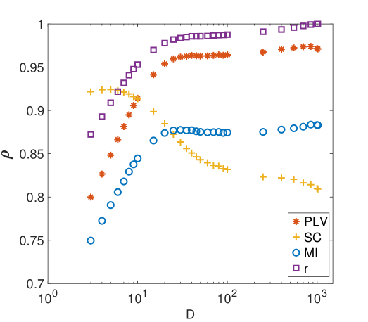
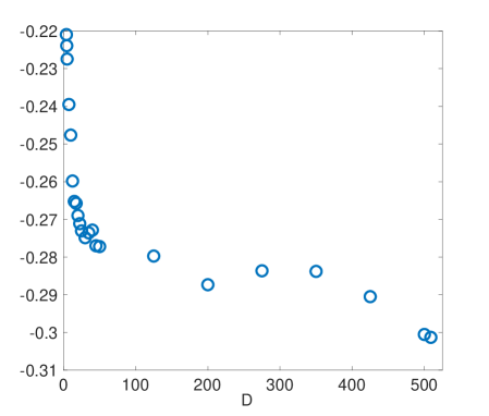
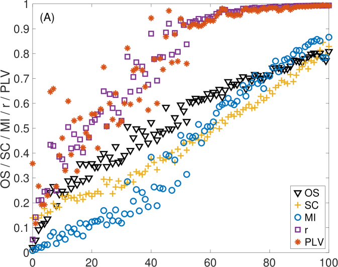
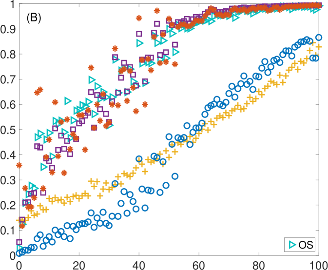
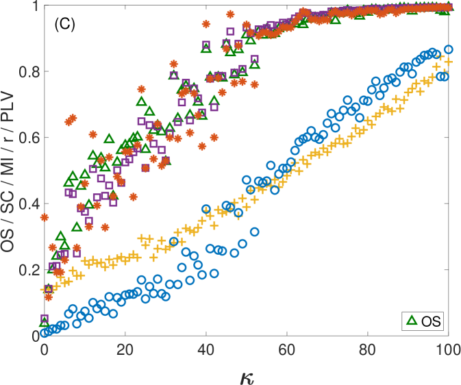
The second application is the evaluation of the level of synchronization between the 241 sensors measuring the activity of an individual during resting state. Concretely, we have 30 recordings of 2 minutes each. In this case, we can not control the amount of coupling between sensors but, alternatively, we have a diversity of levels of synchronizations between all possible pairs of sensors. Figure 5 shows how the correlations between and the rest of the metrics change depending on . As we can observe, correlations are high in all cases except for SC, but this one saturates around the same as the other synchronizations does.
As in the case of the electronic Lorenz oscillators, tuning the value of allows to obtain values of closer, or more correlated, to other metrics. In fact, two different regions are clearly observed: (i) for values of the correlation of with PLV, r, and MI increases with , while (ii) for correlation saturates around the highest value, being the metric with the highest correlation. Interestingly, the behaviour of the SC goes in the opposite direction, decreasing for higher values of .
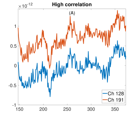
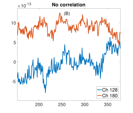
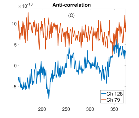
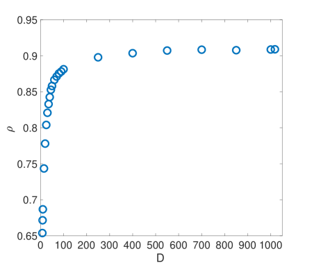
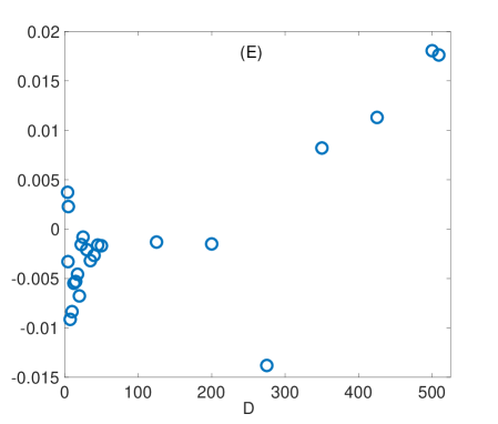
In order to gain insights about how the behaviour of depends on the level of synchronization and the length , we plot three different cases in Figure 6. In (A), we show the time series of two highly-correlated sensors, with their corresponding value depending on (Fig. 6D). Plot (B) and (C) show the cases of two uncorrelated and negatively correlated sensors, respectively, with their values of (Fig. 6E and F). Note that for the positive (negative) case, correlations tend to stabilize as grows, indicating the existence of a certain temporal scale at which synchronization is increased (reduced). Also note that, when time series are not correlated, this pattern is not that clear, and values remain low for any value of .
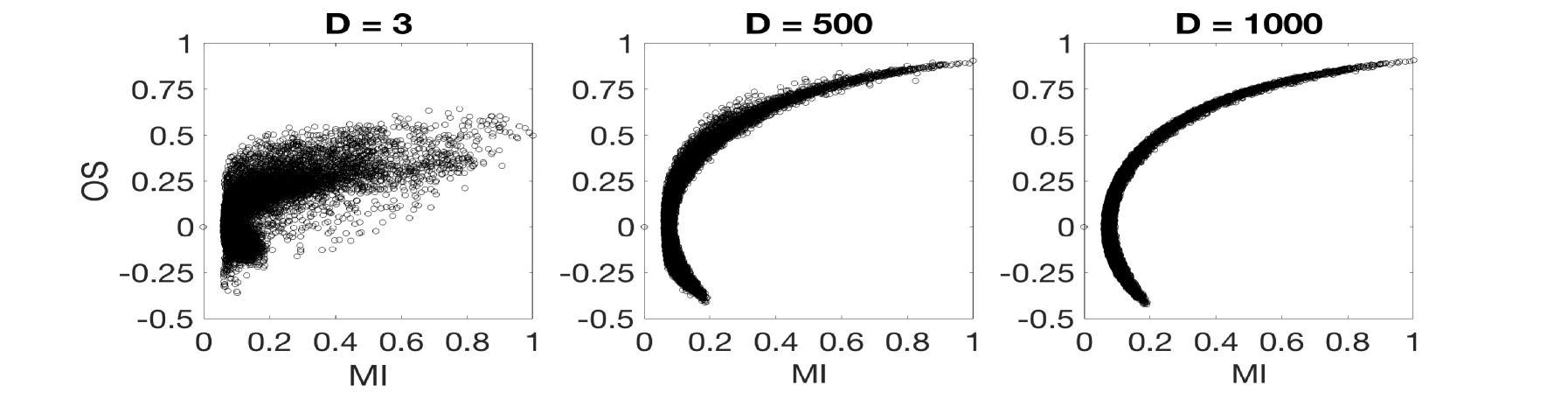
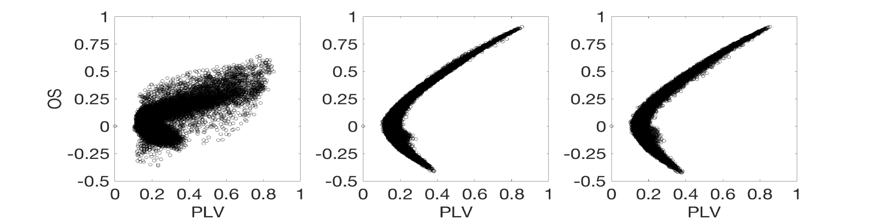
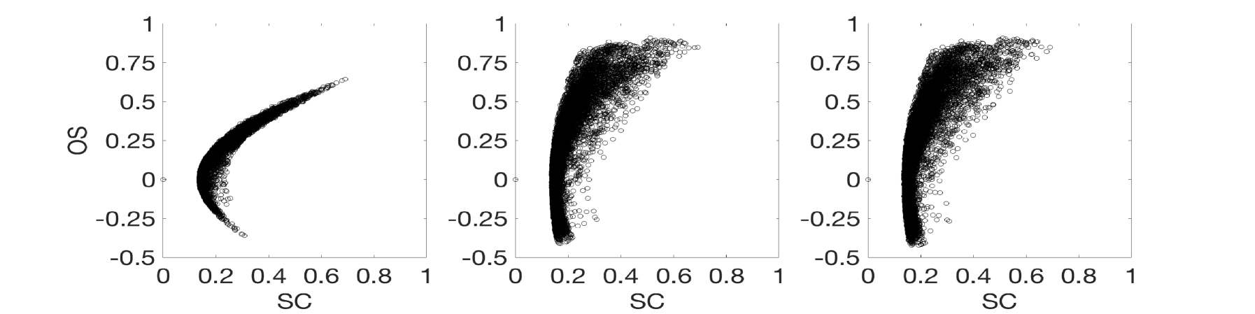
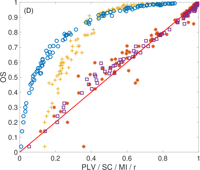
We had analyzed the relation of with the rest of the metrics according to the level of synchronization. Figure 7 shows a panel of plots capturing the correlations between and all other synchronization metrics for the MEG signals. Left plots show the case of , middle plots show and right plots show . Different conclusions can be drawn depending on the synchronization metric is compared to. In the case of (first row), the existence of a nonlinear correlation between both metrics arises. However, this correlation decreases with the length of the ordinal vectors, becoming rather noisy for . This behaviour is induced by the intrinsic noise of the MEG signals that, as in the case of electronic circuits, affects the value of when short lengths of the ordinal vectors are considered. Also note that is not able to distinguish positive from negative correlations between time series, a fact that makes an interesting metric when both kind of synchronizations are expected. In our case, for example, despite the highest values of are close to , the lowest ones arrive to , indicating the existence of anti-correlated dynamics between certain pairs of sensors. A similar behaviour is reported in the case of the comparison with (second row). Again, a nonlinear relation exists between both metrics, which is rather noisy at low values of the ordinal vector lengths (). has also the same limitations as , since it does not differentiate between positive and negative correlations. Interestingly, the relation with is different from the two previous metrics (third row). Despite a nonlinear correlation between and seems to be present in the plots, this correlation is deteriorated with the increase of .
Finally, shows a clear linear correlation with (bottom row), which, as in the case of and becomes noisy for low values of . Note that, the loss of correlation for low values of is indicating that, at short time scales, is capturing a different pattern of synchronization than at large scales. This is an interesting feature of which suggests that, when using it as a metric to evaluate synchronization between signals, it is appealing to carry out an analysis depending on the vector length in order to reveal the existence of different levels of synchronization at different time scales.
3 Conclusions
We have introduced the Ordinal Synchronization (), a new metric to evaluate the level of synchronization between time series by means of a projection into ordinal patterns. We have checked the performance of OS with two kinds of experimental data sets obtained from: (i) unidirectionally coupled nonlinear electronic circuits and (ii) 30 magnetoencephalographic recordings containing the signals of 241 channels. There are several advantages of using . First, it is able to capture in-phase and anti-phase synchronization. Second, tuning the length of the ordinal vectors , it is possible to evaluate the level of synchronization at different time scales. Third, it is not necessary to assume any a priori property of the time series, such as stationarity or linear coupling. Fourth, the calculation of is extremely fast, especially when compared with other metrics such as . On the other hand, we have also seen that one of the elements affecting the value of is the existence of noise, which reduces its value if the dimension of the ordinal vectors is low. However, depending on the application, this fact can also be considered as an indicator of the existence of noise.
A comparison with other classical metrics to evaluate synchronization has been carried out showing some similarities and differences. In general, shows high correlation with and , something that can be explained by the way is constructed. Ordinal patterns filter part of the information contained in the amplitude of the signal, maintaining just the ranking in the time series. This is something between considering just the phase () or just the amplitude (), since differences in amplitude are not related to changes in the parameter as long as the ranking is not modified.
In view of all, we believe that the use of can be interesting (but not restricted to) for evaluating the amount of synchronization in neuroscientific data sets, where in-phase and anti-phase synchronization are know to co-exist, together with coordinations at different time scales.
Appendix A: Coordination metrics
A.1. Pearson’s Correlation Coefficient
The Pearson’s correlation coefficient consists of a covariance scaled by variances, thus capturing linear relationships among variables. From the equations of the variance (of and ) and covariance (of ), we obtain Pearson Correlation Coefficient as:
| (10) | ||||
| (11) | ||||
| (12) | ||||
| (13) |
Pearson’s correlation is a measure of linear dependence between any pair of variables and it has the advantage of not requiring the knowledge of how variables are distributed. However, it should be applied only when variables are linearly related to each other.
A.2. Coherence
Coherence (magnitude squared coherence or coherence spectrum) measures the linear correlation among the two spectra[12]. To calculate the coherence spectrum, data must be in the frequency domain. In order to do so, time series are usually divided into S sections of equal size. The Fast Fourier Transform algorithm is then computed over the sections to get the estimate of each section’s spectrum (periodogram). Then, the spectra of the sections is averaged to get the estimation of the whole data’s spectrum (Welch’s method). Finally, Coherence is a normalization of this estimate by the individual autospectral density functions [12]:
| (14) |
where is the Cross Power Spectral Density (CPSD) of both signals, and are the Power Spectral Density (PSD) of the segmented signals and taken individually, and is the average over the S segments. In the case of the data sets obtained with the nonlinear electronic Lorenz systems, frequencies higher than Hz have been disregarded for the computation of , since the power spectra of the electronic circuits are completely flat above this frequency. One of the drawbacks of Coherence is that it doesn’t discern the effects of amplitude and phase in the relationships measured between two signals, which makes its interpretation unclear [23, 4].
A.3. Phase Locking Value
Phase Locking Value was first introduced by Lachaux et al. [23] as a new method to measure synchrony among neural populations. It has, at least, two major advantages over the classical coherence measure: it doesn’t require data to be stationary, a condition that can rarely be validated; and has a relatively easy interpretation (in terms of phase coupling). However, the methods used to extract instantaneous phase, a step needed to calculate rely on stationarity, so indirectly can be affected by this condition [24]. To obtain the , the signal has to be decomposed to it’s instantaneous phases and amplitudes. To achieve this, there are several methods, such as Morlet wavelet convolution or Hilbert transform [12, 24]. In this work we will utilize the latter. Finally, is obtained averaging over time :
| (15) |
where is the (instantaneous) phase difference , the phases to be compared from the signals and . Comparisons are carried out pairwise (bivariate).
A.4. Mutual Information
Mutual Information is a measure of shared information between any components of a system, between systems, or any other parameter whose value’s probability can be estimated. It is based on Shannon’s notion of entropy, which, in a general sense, tries to quantify the amount of information contained in a random variable by means of its estimated probability distribution. Mutual information measures the amount of information shared between two random variables by means of its joint distribution, or conversely, the amount of information we can obtain from one random variable observing another. This is analogue to measuring the dependence between two random variables [25]. Let X and Y be two random variables with and , possible values with probabilities and . The of X relative to Y can be written as:
| (16) |
| (17) |
where is the probability that has a value of while has a value of , is the entropy of and is the conditional entropy of and . One of the major advantages of is that it captures linear and non-linear relationships among variables. One disadvantage is that it does not explicitly tell the shape of that distribution [24]. To get the mutual information between two random variables, we first need to estimate their probability density distribution [25, 24, 26]. Equation 16 compares joint probabilities against marginal ones. When two values are independent, the product of their marginal probabilities should equal their joint probability. When not, we can state that there is a relationship among them (not necessarily linear), because the probability of finding those values together is greater than the probability of finding them by chance. Thus, somehow, those time series are coupled, although we don’t know the way it occurs.
Appendix B: Electronic version of the Lorenz system
The equations of the master and slave electronic Lorenz systems are:
| (18) | |||
| (19) | |||
| (20) | |||
| (21) | |||
| (22) | |||
| (23) |
where , and are the voltage variables of the master (sub-index 1) and slave (sub-index 2) Lorenz systems, is the coupling signal injected into the slave system in a diffusive way, is the coupling strength and is the percentage of coupling controlled by the digital potentiometer. In the experiments where external noise is considered (see Appendix C), the amplitude of and are set to V and zero otherwise.
Table 1 contains the parameters of the resistances and capacitances used in the experiments.
| [0-1] | ||
Appendix C: Robustness of in the presence of external noise
Figures 8-9 are equivalent to Figs. 3-4 but in the presence of external noise. In this case, we have introduced two noises and perturbing the and variables of the master and slave Lorenz systems as explained in Appendix B. Comparing Fig. 8 and Fig. 3 we can observe that all synchronization metrics have reduced their values in the presence of external noise, however, the behaviour remains qualitatively similar to the one reported in Fig. 3. Again, the case is the one suffering the most from the presence of noisy signals (Fig. 8D). When comparing with the rest of synchronization metrics (Fig. 9), we can also observe a reduction of the correlations respect to the case without external noise. Again, and are the metrics showing higher correlation with , having a linear correlation for and . This correlation is impaired for , since it corresponds to the ordinal vector length that is more affected by noise. On the other hand, the nonlinear correlations with and remain quite similar as in the case of the absence of external noise.

References
References
- Huygens [1893] C. Huygens, in oeuvres completes de christian huygens, edited by M. Nijhoff (Societe Hollandaise des Sciences, The Hague, The Netherlands). 5 (1893) 246.
- Néda et al. [2000] Z. Néda, E. Ravasz, Y. Brechet, T. Vicsek, A.-L. Barabási, Self-organizing processes: The sound of many hands clapping, Nature 403 (2000) 849–850.
- Schmidt et al. [1990] R. Schmidt, C. Carello, M. T. Turvey, Phase transitions and critical fluctuations in the visual coordination of rhythmic movements between people, J. Exp. Psychol. Hum. Percept. Perform. 16(2) (1990) 227–247.
- Varela et al. [2001] F. Varela, J. Lachaux, E. Rodriguez, J. Martinerie, The brainweb: phase synchronization and large-scale integration, Nat. Rev. Neurosci. 2 (2001) 229–239.
- Agladze et al. [2017] N. Agladze, O. Halaidych, V. Tsvelaya, T. Bruegmann, C. Kilgus, P. Sasse, K. Agladze, Synchronization of excitable cardiac cultures of different origin, Biomater. Sci. 5 (2017) 1777.
- Romer [2001] K. Romer, Time synchronization in ad hoc networks, in: Proceedings of ACM Symposium on Mobile Ad Hoc Networking and Computing (MobiHoc) (2001) 173–182.
- Wang et al. [2016] B. Wang, H. Suzuki, K. Aihara, Enhancing synchronization stability in a multi-area power grid, Sci. Rep. 6 (2016) 26596.
- Arenas et al. [2008] A. Arenas, A. Díaz-Guilera, J. Kurths, Y. Moreno, C. Zhou, Synchronization in complex networks, Phys. Rep. 469 (2008) 93–153.
- Boccaletti et al. [2006] S. Boccaletti, V. Latora, Y. Moreno, M. Chavez, D. U. Hwang, Complex networks: Structure and dynamics, Phys. Rep. 424 (2006) 175–308.
- Mones et al. [2014] E. Mones, N. Araújo, T. Vicsek, H. Herrmann, Shock waves on complex networks, Sci. Rep. 4 (2014) 4949.
- Rech and Perret [1990] C. Rech, R. Perret, Adding dynamics to the Human Connectome Project with MEG, Int. J. Syst. Sci. 21 (1990) 1881.
- Pereda et al. [2005] E. Pereda, R. Q. Quiroga, J. Bhattacharya, Nonlinear multivariate analysis of neurophysiological signals, Progress in Neurobiology 77 (2005) 1–37.
- Bahraminasab et al. [2008] A. Bahraminasab, F. Ghasemi, A. Stefanovska, P. McClintock, H. Kantz, Direction of coupling from phases of interacting oscillators: A permutation information approach, Phys. Rev. Lett. 100 (2008) 084101.
- Paluš and Stefanovska [2003] M. Paluš, A. Stefanovska, Direction of coupling from phases of interacting oscillators: An information-theoretic approach, Phys. Rev. E 67 (2003) 055201.
- Li et al. [2011] Z. Li, G. Ouyang, D. Li, X. Li, Characterization of the causality between spike trains with permutation conditional mutual information, Phys. Rev. E 84 (2011) 021929.
- Izhikevich [2003] E. Izhikevich, Simple model of spiking neurons, IEEE Trans. Neural Netw. 14 (2003) 1569.
- Rosário et al. [2015] R. Rosário, P. Cardoso, M. Muñoz, P. Montoya, J. Miranda, Motif-synchronization: A new method for analysis of dynamic brain networks with eeg, Physica A 439 (2015) 7–19.
- Olofsen et al. [2008] E. Olofsen, J. Sleigh, A. Dahan, Permutation entropy of the electroencephalogram: a measure of anaesthetic drug effect, Br. J. Anaesth. 101 (2008) 810–821.
- Bandt and Pompe [2002] C. Bandt, B. Pompe, Permutation entropy: a natural complexity measure for time series., Phys. Rev. Lett. 88 (2002) 174102.
- Lorenz [1963] E. Lorenz, Deterministic nonperiodic flow, J. Atmos. Sci. 20 (1963) 130–141.
- http://zone.ni.com/reference/ [2018] http://zone.ni.com/reference/, National instruments, Noise (2018).
- Larson-Prior et al. [2013] L. Larson-Prior, R. Oostenveld, S. Della Penna, G. Michalareas, F. Prior, A. Babajani-Feremi, J.-M. Schoffelen, L. Marzetti, F. de Pasquale, F. Di Pompeo, J. Stout, M. Woolrich, Q. Luo, R. Bucholz, P. Fries, V. Pizzella, G. Romani, M. Corbetta, A. Snyder, Adding dynamics to the Human Connectome Project with MEG, NeuroImage 80 (2013) 190–201.
- Lachaux et al. [1999] J. P. Lachaux, E. Rodriguez, J. Martinerie, F. J. Varela, Measuring Phase Synchrony in Brain Signals, Human Brain Mapping 8 (1999) 194–208.
- Cohen [2014] M. X. Cohen, Analyzing Neural Time Series Data: Theory and Practice, MIT Press, Cambridge, Massachusetts, 2014.
- Veyrat-Charvillon and Standaert [2009] N. Veyrat-Charvillon, F.-X. Standaert, Mutual Information Analysis: How, When and Why?, Cryptographic Hardware and Embedded Systems-CHES 2009. Lecture Notes in Computer Science (LNCS) 5747 (2009) 429–443.
- Gierlichs et al. [2008] B. Gierlichs, L. Batina, P. Tuyls, B. Preneel, Mutual Information Analysis A Generic Side-Channel Distinguisher, Cryptographic Hardware and Embedded Systems-CHES 2008. Lecture Notes in Computer Science 5154 (2008) 426–442.