[2]\fnmMomoko \surHayamizu
1]\orgdivDepartment of Pure and Applied Mathematics, \orgnameGraduate School of Fundamental Science and Engineering, Waseda University, \countryJapan
2]\orgdivDepartment of Applied Mathematics, Faculty of Science and Engineering, \orgnameWaseda University, \countryJapan
Orientability of Undirected Phylogenetic Networks to a Desired Class: Practical Algorithms and Application to Tree-Child Orientation
Abstract
The -Orientation problem asks whether it is possible to orient an undirected graph to a directed phylogenetic network of a desired network class . This problem arises, for example, when visualising evolutionary data, as popular methods such as Neighbor-Net are distance-based and inevitably produce undirected graphs. The complexity of -Orientation remains open for many classes , including binary tree-child networks, and practical methods are still lacking. In this paper, we propose an exact FPT algorithm for -Orientation that is applicable to any class and parameterised by the reticulation number and the maximum size of minimal basic cycles, and a very fast heuristic for Tree-Child Orientation. While the state-of-the-art for -Orientation is a simple exponential time algorithm whose computational bottleneck lies in searching for appropriate reticulation vertex placements, our methods significantly reduce this search space. Experiments show that, although our FPT algorithm is still exponential, it significantly outperforms the existing method. The heuristic runs even faster but with increasing false negatives as the reticulation number grows. Given this trade-off, we also discuss theoretical directions for improvement and biological applicability of the heuristic approach.
keywords:
Phylogenetic Networks, Tree-Child Networks, Acyclic Graph Orientation, FPT Algorithm, Exact Algorithm, Heuristic Algorithm1 Introduction
Phylogenetic networks are a powerful tool for representing complex evolutionary relationships between species that cannot be adequately modelled by trees. These networks are particularly useful in the presence of reticulate events, such as hybridisation, horizontal gene transfer (HGT) and recombination. Hybridisation refers to the interbreeding of individuals from different species, which can lead to the formation of a new hybrid species that shares genetic material from both parent species. HGT is the transmission of copied genetic material to another organism without being its offspring, a process particularly common in bacteria and archaea. Recombination is the exchange of genetic material between different genomes and is a common occurrence not only in viruses but also in bacteria, eukaryotes, and other organisms. While phylogenetic trees depict the hierarchical branching of evolutionary lineages, networks can represent both the hierarchical and non-hierarchical connections resulting from reticulate events, providing a more nuanced view of evolutionary history.
However, constructing directed phylogenetic networks from biological data remains a challenging task. Distance-based methods, such as Neighbor-Net, are widely used because they are scalable and helpful in visualising the data. However, the resulting networks are inevitably undirected, often making it difficult to interpret the evolutionary history. To provide a more informative representation of the data, it is meaningful to develop a method for transforming undirected graphs into directed phylogenetic networks in a way that ensures the resulting network has a desired property.
Recently, Huber et al. [1] introduced two different orientation problems, each considering orientation under a different constraint. The Constrained Orientation problem asks whether a given undirected phylogenetic network can be oriented to a directed network under the constraint of a given root edge and desired in-degrees of all vertices, and asks to find a feasible orientation under that constraint if one exists. In [1], it was shown that such a feasible orientation is unique if one exists, and a linear time algorithm for solving this problem was provided. However, when an undirected network has been created from data, it is not usually the case that there is complete knowledge of where to insert the root and which vertices are reticulations. The -Orientation problem does not constrain the position of the root or the in-degree of the vertices. Instead, it asks whether a given binary network can be oriented to a directed phylogenetic network belonging to a desired class .
The complexity of -Orientation is not fully understood for many classes , and no study has discussed practically useful methods. In [1], Tree-Based Orientation was shown to be NP-hard. Maeda et al. [2] conjectured that Tree-Child Orientation is NP-hard. Bulteau et al. [3] studied a similar problem and showed that for a graph with maximum degree five, determining whether the graph can be oriented to a tree-child network with a designated root vertex is NP-hard (Corollary 5 in [3]). Without the assumption of maximum degree five, the complexity of this problem is still unclear. Indeed, [3] was concluded by noting that even for graphs of maximum degree three (i.e. binary networks), finding an orientation to a desired class, such as tree-child, tree-based or reticulation-visible networks, may not be easy. Although [1] provided FPT algorithms for a special case of -Orientation where satisfies several conditions, which are theoretically applicable to various classes including tree-child networks but are not easy to implement, there is no FPT algorithm to solve -Orientation in its general form. Also, no studies have pursued practically useful heuristics.
In this paper, we provide a practically efficient exponential time algorithm for -Orientation (Algorithm 1), which is FPT in both the reticulation number and the maximum size of minimal basic cycles selected by the algorithm. We also present a heuristic method for Tree-Child Orientation (Algorithm 2) which, although still exponential, runs very fast in practice because it only considers reticulation placements to maximise the sum of their pairwise distances. Using artificially generated networks, we compare the accuracy and execution time of the proposed methods for solving Tree-Child Orientation with those of the existing exponential time algorithm for -Orientation (Algorithm 2 in [1]). Our theoretical and empirical results demonstrate the usefulness of Algorithm 1, especially for relatively large input graphs with or more reticulations, where the exponential time method in [1] becomes computationally infeasible. Our Algorithm 2, while much faster than Algorithm 1, tends to decrease in accuracy as the reticulation number increases.
The rest of the paper is structured as follows. Section 2 provides the necessary mathematical definitions and notation, including the definition of phylogenetic networks. Section 3 briefly reviews relevant results from [1] and formally states the problems of interest. Section 4 gives the theoretical background of our proposed methods, including the concept of ‘cycle basis’ and a theorem that allows us to reduce the search space (Theorem 4). Section 5 describes the proposed exact method (Algorithm 1) and a heuristic method (Algorithm 2). Theorem 7 ensures that the heuristic is correct when . We analyse the time complexity of Algorithm 1. Section 6 explains the experimental setup, including the method used to create undirected graphs (details can be found in the appendix), and presents the results of three experiments. Section 7 discusses the limitations and biological application of the heuristic method. Finally, Section 8 concludes the paper and outlines future research directions.
2 Definitions and Notation
2.1 Graph theory
An undirected graph is an ordered pair consisting of a set of vertices and a set of edges between vertices without any orientation. Given an undirected graph , its vertex set and edge set are denoted by and , respectively. An edge of an undirected graph between vertices and is denoted by or . An undirected graph is simple if it contains neither a loop nor multiple edges, namely, any edge satisfies , and any edges satisfy at least one of and . Given simple graphs (), the graph with and is called the union of the graphs .
For a vertex of an undirected graph , the degree of in , denoted by , is the number of edges of that joins with another vertex of .
An (undirected) path is an undirected graph with a vertex set and an edge set . The number of edges of a path is called the length of . An (undirected) cycle is an undirected graph with a vertex set and an edge set . The number of edges of a cycle is called the length of . A subgraph of an undirected graph is a graph such that and . In this case, contains . If an undirected graph contains a cycle as a subgraph, is a cycle of . An undirected graph is connected if for any , contains a path between and . The distance between and in is defined by the length of the shortest path connecting and in .
A directed graph is an ordered pair consisting of a set of vertices and a set of oriented edges called arcs. Given a directed graph , its vertex set and arc set are denoted by and , respectively. An arc that goes from vertex to vertex is denoted by . Given an arc , is a parent of and is a child of . A directed graph is simple if it contains neither a loop nor multiple arcs. For a vertex of a directed graph , the in-degree of in , denoted by , is the number of arcs of that arrive at . Likewise, the out-degree of in , denoted by , is the number of arcs of that start from . A directed cycle is a directed graph with a vertex set and an arc set . A subgraph of a directed graph is defined in the same way as before. A directed acyclic graph (DAG) is a directed graph that contains no cycle as its subgraph. Given a directed graph , the undirected graph obtained by ignoring the direction of all its arcs is called the underlying graph of and denoted by .
2.2 Phylogenetic networks
Throughout this paper, is a finite set with , representing a set of the present-day species of interest. All graphs considered here are simple and finite, meaning the numbers of vertices and edges are finite. An undirected binary phylogenetic network on is a simple, connected, undirected graph such that its vertex set is partitioned into and , and can be identified with . Each vertex in and in is called an internal vertex and a leaf of , respectively.
A directed binary phylogenetic network on is a simple, acyclic directed graph such that the underlying graph of is connected, the vertex set of contains a unique vertex with and the set is partitioned into and , and that can be identified with . The vertex is called the root of , and each vertex in , in and in is called a tree vertex, a reticulation and a leaf of , respectively.
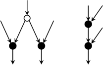
A directed binary phylogenetic network on is a tree-child network if every non-leaf vertex of has at least one tree vertex as a child [4]. Tree-child networks are characterised by the absence of the two forbidden subgraphs [5] that are illustrated in Fig. 1. Namely, tree-child networks contain neither a vertex with two reticulation children nor a reticulation with a reticulation child.
3 Acyclic orientation problems and known results
For an undirected phylogenetic network on , orienting is a procedure that inserts the root into a unique edge of by replacing the edge with the arcs and then orienting the other edges so that the resulting graph is a directed phylogenetic network on . In other words, a directed phylogenetic network on is an orientation of if the underlying graph becomes isomorphic to after suppressing the root of (i.e. replacing the undirected path with the edge ).
Determining the orientability of undirected graphs to directed graphs with desired properties is a classic topic in graph theory and its application (e.g. [6]), but orientability problems for phylogenetic networks have only recently been studied [1, 3]. Huber et al. [1] discussed two types of problems, Constrained Orientation and -Orientation.
3.1 Orientation with a desired root position and in-degrees
Problem 1.
(Constrained Orientation)
- INPUT:
-
An undirected (not necessarily binary) phylogenetic network on , an edge into which a unique root is inserted, and the desired in-degree of each .
- OUTPUT:
-
An orientation of that satisfies the constraint if it exists, and ‘NO’ otherwise.
We note that when is binary, the constraint in Problem 1 specifies which internal vertices of are to become reticulations or tree vertices in . Below we restate the relevant result from [1].
Theorem 1 (Part of Theorems 1 and 2 in [1]).
3.2 Orientation to a desired class of networks
The next problem is about orientation under a different constraint. It asks whether a given graph can be oriented to be a directed phylogenetic network in a desired class , where the position of the root edge and the in-degree of each vertex are unknown. In [1], -Orientation was defined under the assumption that the input is binary, unlike Problem 1.
Problem 2.
(-Orientation)
- INPUT:
-
An undirected binary phylogenetic network on .
- OUTPUT:
-
An orientation of such that belongs to the class of directed binary phylogenetic networks on if it exists, and ‘NO’ otherwise.
Huber et al. [1] described a simple exponential time algorithm for solving Problem 2 (Algorithm 2 in [1]), which uses the above-mentioned time algorithm for Problem 1. It repeatedly solves Problem 1 for all possible combinations of the root edge and a set of reticulations (i.e. vertices of desired in-degree ) until it finds an orientation of that satisfies and belongs to class .
The complexity of -Orientation depends on but is still unknown for most of the popular classes of phylogenetic networks. For example, when is the class of trees, Problem 2 is obviously solvable in polynomial time, and when is the class of tree-based networks, it was shown in [1] that the problem is NP-hard. An important remark is that if is a subclass of , it does not necessarily imply that -Orientation is easier or harder than -Orientation. In fact, the complexity of the following problem is still open [7, 8].
Problem 3.
(Tree-Child Orientation)
- INPUT:
-
An undirected binary phylogenetic network on .
- OUTPUT:
-
An orientation of that is a tree-child network on if it exists, and ‘NO’ otherwise.
While FPT algorithms for a special case of -Orientation were provided in [1], it remains challenging to develop a practical method for this type of orientation problems. This motivates us to explore a heuristic approach for solving Problem 3.
In what follows, when there exists such an orientation of as described in Problem 3, we say that is tree-child orientable and call a tree-child orientation of .
4 Theoretical aspects of the proposed methods
Before discussing Problem 3, we consider a general setting where we want to orient any undirected phylogenetic network on to a rooted directed phylogenetic network on . Then must contain reticulation vertices (which can be easily verified by induction, and can also be derived from the equations in Lemma 2.1 in [9]), and so we need to decide which vertices among internal vertices of will have in-degree 2 in . The number of possible ways to select vertices from non-leaf vertices of is , which is exponential. We will now consider how we can reduce the number of candidates to examine.
Lemma 2.
Let be any directed acyclic graph and let be the underlying graph of . Then, any cycle of has a vertex whose in-degree in is at least .
Proof.
To obtain a contradiction, suppose contains a cycle such that for every . Let be the subgraph of that corresponds to . If contains with , then must contain another vertex with . Then, for each , holds. Let and be two consecutive undirected edges of . We may assume that has the arc , instead of . Since , contains , not . The same argument applies to all arcs of . It follows that is a directed cycle, a contradiction. ∎
Lemma 2 allows us to exclude some of the inappropriate reticulation placements (specifically, cases where there is a cycle having no reticulation) that make orientation impossible. However, checking all cycles in a graph is computationally inefficient. To reduce the search space, we will now introduce some relevant concepts.
For a connected undirected graph , the cycle rank of is defined to be the number (e.g. p.24 in [10]), which is also known as circuit rank, cyclomatic number and the (first-order) Betti number of . Note that is zero if is a tree and that is the number of desired reticulation vertices if is a binary phylogenetic network that is an instance of Problem 1. The cycle rank of can also be interpreted as the rank of a vector space called the ‘cycle space’, where each of the basis vectors, called a basic cycle, corresponds to the edge-set of a simple cycle in . If we define the summation of cycles and as the cycle induced by the symmetric difference of their edge-sets, then the cycle space of can be identified with the set of even-degree subgraphs of , so any cycle in can be expressed as a sum of basic cycles in a cycle basis (for details, see Section 1.9 of [11], Section 4.3 of [12] and Section 6.4.2 of [10]).
Proposition 3.
Let be any directed graph. If each satisfies , then holds, where and (resp. ) denotes the set of vertices with (resp. ). If, in addition, is acyclic, then holds.
Proof.
Let . Since the sum of in-degrees of all vertices must equal , we have . Hence, .
We claim holds if is acyclic. To verify this, we will prove that any finite directed acyclic graph has at least one vertex of in-degree zero. Let be a longest vertex-disjoint directed path in , with and as the start and end vertices of , respectively. If , there exists a vertex with . Since is acyclic, is not a vertex of . Then, by adding to , one can obtain a vertex-disjoint directed path in that is longer than , but this contradicts the maximality of . Thus, holds, which proves the above claim. Hence, we obtain . ∎
Theorem 4.
Let be an instance of Problem 1 where is binary and let denote the set of reticulations specified by . If there exists an orientation of satisfying the constraint , then for any cycle basis of , there exists a bijection with the property that holds for each .
Proof.
Let be any cycle basis of and let be the bipartite graph defined by and . Here, holds (note that we could have if were allowed to have a reticulation with a large in-degree but here is binary). We also see that no vertex of has degree zero for the following reasons: since is a directed acyclic graph, Lemma 2 implies that for each cycle , there exists at least one reticulation with ; conversely, for each reticulation , there exists at least one cycle with . The proof will be completed if we can show that there is a perfect matching in . We will prove that satisfies the marriage condition, i.e. for any subset of , holds, where is the neighbourhood of in . To prove this, without loss of generality, we may assume that the union of all cycles in , denoted by , is a connected subgraph of .
Recalling that is a unique acyclic orientation for , one can convert into a directed graph by assigning the same direction to each edge of as in . Since is a subgraph of , is also acyclic. By construction, each vertex of satisfies . If we write for the set , then Proposition 3 yields . The left hand side equals . Since the in-degree of a vertex in a subgraph never exceeds its in-degree in the original graph , we have . Thus, holds. Hence, by Hall’s marriage theorem, has a perfect matching. Any perfect matching in induces a bijection satisfying for each . ∎
Theorem 4 provides a necessary condition for the feasibility of a reticulation placement in Problem 1 (binary version), where feasibility means that admits an acyclic orientation for some . This implies that we need not consider all reticulation placements in solving Problem 2, regardless of the class we are interested in. Therefore, we may use an arbitrary cycle basis of and choose exactly one reticulation vertex from each of the basic cycles, thereby reducing the search space for feasible reticulation placements in both Problems 2 and 3.
In solving Problem 3, we will also use the following results. From the forbidden structures of tree-child networks (Fig. 1), Lemma 5 follows immediately, and this leads to Theorem 6.
Lemma 5.
A directed phylogenetic network is tree-child if every two reticulations of are distant at least in the underlying graph of .
Theorem 6.
If is an instance of Problem 1 such that for any distinct and if there exists an orientation of that satisfies the constraint , then is a tree-child network.
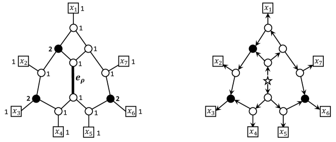
We note that Theorem 6 provides a sufficient condition for tree-child orientability, not a necessary condition. In fact, a tree-child network can contain a pair of reticulations whose distance is less than 3 (see Fig. 2).
5 Proposed methods
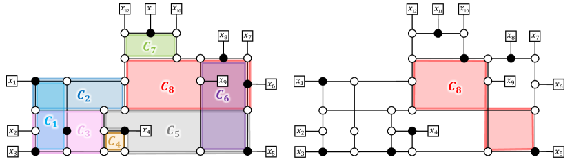
Based on Theorem 4, we propose an exact method (Algorithm 1) for -Orientation (Problem 2) and a heuristic method (Algorithm 2) for Tree-Child Orientation (Problem 3). While Theorem 4 holds for any cycle basis, our algorithms use a ‘minimal’ one for computational efficiency. A cycle basis of is called minimal if the sum of the lengths of all cycles in is not greater than that of any other cycle basis of , i.e. minimising . Intuitively, focusing on a minimal cycle basis allows us to use basic cycles that do not overlap too much. The problem of computing a minimal cycle basis has been extensively studied (e.g. [13, 14, 15]; see Chapter 7 of [16] for a brief literature review) and polynomial time algorithms exist (e.g. [16, 17, 15]). By using an algorithm given in [17], a minimal cycle basis of can be computed in .
For both Problems 2 and 3, our proposed methods first compute a minimal cycle basis of a given network . Then, for Problem 2, our exact method (Algorithm 1) repeatedly picks exactly one reticulation vertex from each basic cycle to obtain a candidate set of reticulations, and solves Problem 1 for all until it finds a -orientation of . While this algorithm still requires exponential time, it is more efficient than the exponential time method in [1] because the search space for appropriate is smaller than .
For Problem 3, we first note that a straightforward way to reduce the search space for is to exclude any candidate sets containing adjacent reticulations, as such configurations are invalid in tree-child networks (recall Fig. 1, right panel). Beyond this basic constraint, we introduce a novel approach to further reduce the search space based on Theorem 6, which suggests that reticulations should be placed as far apart as possible. This insight leads to our heuristic method (Algorithm 2) that considers only those reticulation sets that maximise the sum of pairwise distances between reticulations. While this significant reduction in the search space makes the algorithm faster than Algorithm 1, it may fail to find an existing tree-child orientation; more precisely, while false positives cannot occur, a ‘NO’ output from Algorithm 2 should be interpreted as ‘Probably NO’. However, Theorem 7 ensures that Algorithm 2 works correctly when is very small.
Theorem 7.
Proof.
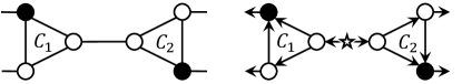
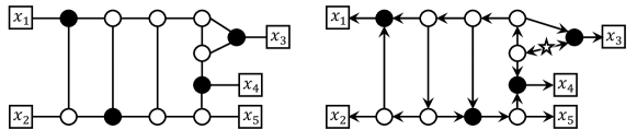
We may focus on the case of as the statement is obvious when . Then, contains exactly two cycles and , each of which has at least edges.
When and do not share an edge, is a level- network. This implies that is planar and tree-child orientable (see Fig. 3). Algorithm 2 computes a minimal cycle basis of , which is unique in this case. Then, Algorithm 2 selects a most distant pair in . Since is binary, . We can see that has an orientation for the root edge shown in Fig. 3. By Theorem 6, is tree-child. Hence, Algorithm 2 can correctly find a tree-child orientation of .
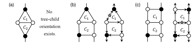
When and share an edge, they share exactly one edge because otherwise. Then, as Fig. 4 indicates, has a tree-child orientation if and only if at least one of and has or more edges. When each of and has exactly edges as in Fig. 4(a), Algorithm 2 correctly returns ‘NO’. When and , the algorithm selects a most distant pair in as in Fig. 4(b). Although holds, the algorithm can insert the root into an appropriate edge , making their distance from into . When and as in Fig. 4(c), . Hence, when a tree-child orientation of exists, Algorithm 2 correctly outputs it. ∎
Theorem 8 states that Algorithm 1 is FPT both in the reticulation number and the size of longest basic cycles in used in the computation.
Theorem 8.
Proof.
Recalling a minimal cycle basis of can be computed in time by the algorithm in [17], we know that Line 2 takes time. Line 5–7 takes time for each . Also, since one can check in time whether or not is in the class of tree-child networks, Line 8–14 takes time for each . Line 5–14 needs to be repeated times. Therefore, Line 4–15 can be done in time. Since is binary, holds. Thus, Algorithm 1 runs in time. ∎
Theorem 8 implies that the unparameterised worst-case complexity of Algorithm 1 is . This complexity is equivalent to that of the exponential time method (Algorithm 2 in [1]) that performs time calculations for all reticulation placements. Although two FPT algorithms for a special case of -Orientation were proposed in [1], Algorithm 1 differs in its parameterisation from them. Specifically, our Algorithm 1 is parameterised by and , while the FPT algorithms in [1] are parameterised by and by the level of , respectively.
Theorem 8 also shows that the size of search space depends on the choice of at Line 2 of Algorithm 1 although never exceeds the size of longest cycles in (the same applies to Line 2 of Algorithm 2). To illustrate this, consider two minimal cycle bases with and where , and (note that they have the same total length ). When the former is selected, the number of elements of at Line 3 of either algorithm is , whereas for the latter .
6 Experiments
We implemented our two proposed methods (Algorithms 1 and 2) and the existing exponential time algorithm described by Huber et al. (Algorithm 2 in [1]) using Python 3.11.6. In the implementation of Algorithms 1 and 2, we used the minimum_cycle_basis function from the Python package networkx to compute a minimal cycle basis. We note that the algorithm implemented in networkx is not the algorithm given in [17] but the algorithm given in Section 7.2 of [16]. Undirected binary phylogenetic networks were generated as test data using a method described in Appendix. The source code, test data, and the program used to generate the data are available at https://github.com/hayamizu-lab/tree-child-orienter. The full details of the results can be found at https://github.com/hayamizu-lab/tree-child-orienter/tree/main/results.
6.1 Experiment 1: Execution time
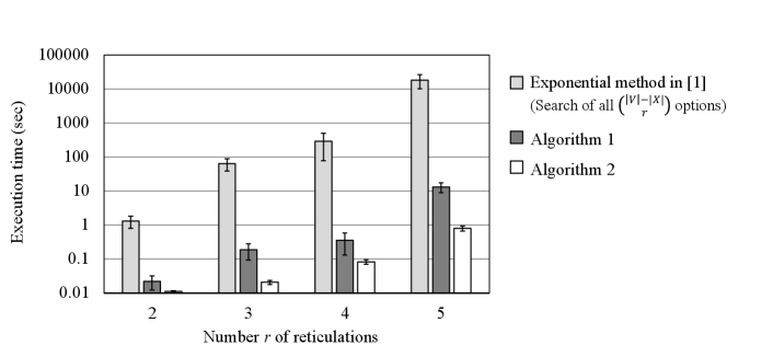
In Experiment 6.1, we compared the execution times of the following methods: the existing exponential time algorithm (Algorithm 2 in [1]), Algorithm 1, and Algorithm 2 on 20 hand-picked tree-child orientable networks with 10 leaves. The 20 networks consisted of five samples each for reticulation numbers and . Due to the time-consuming nature of the existing method, conducting experiments with a larger number of samples was infeasible. The experiment was performed on a MacBook Air (CPU: Intel Core i5, 1.6GHz, 8GB memory). We note that the hardware specification in Experiment 6.1 differs from Experiments 6.2 and 6.3, but this does not undermine the validity of this study as we do not compare results across experiments.
The results are summarised in Fig. 5. Although both Algorithm 2 in [1] and Algorithm 1 require exponential time in general, Algorithm 1 is expected to be faster in practice due to its smaller search space. Indeed, Algorithm 1 was significantly faster than the existing exponential time method. We also confirmed that Algorithm 2 was faster than Algorithm 1.
6.2 Experiment 2: Accuracy for small graphs
In Experiment 6.2, we evaluated the accuracy and execution time of Algorithms 1 and 2 on the 289 networks with 10 leaves and 1 to 5 reticulations in Table 4. The experiment was performed on a MacBook Pro (CPU: Apple M2 Pro, clock speed 3.49GHz, memory 16GB). The tree-child orientability of the sample graphs was determined using the existing exponential time algorithm (Algorithm 2 in [1]). Out of 289 instances, 268 were tree-child orientable (YES instances) and 21 were not (NO instances).
The accuracy and execution time of the two methods are summarised in Table 1. The correctness of Algorithm 1 was empirically confirmed, while being much faster than the existing method in [1]. In accordance with Theorem 7, Algorithm 2 returned a correct solution whenever , but in practice, it still worked correctly for most cases with , with a much shorter running time than Algorithm 1 for both YES and NO instances. Algorithm 2 often failed to find a tree-child orientation for YES instances with .
6.3 Experiment 3: Accuracy for large graphs
In Experiment 6.3, we evaluated the performance of Algorithms 1 and 2 on the 471 larger sample networks with 20 leaves and 1 to 9 reticulations in Table 4. The experiment was performed on the same MacBook Pro used in Experiment 6.2. Since Algorithm 2 in [1] became infeasible for most cases with , we compared Algorithms 1 and 2 based on the number of tree-child orientations found and the time taken to find one.
The results are summarised in Table 2. As reticulation number increased, the ability of Algorithm 2 to find tree-child orientations decreased monotonically. By contrast, Algorithm 1 was still able to find a tree-child orientation for many instances with large . It generally takes a long time, but sometimes it can find a tree-child orientation in a practical time.
| Algorithm 1 | Algorithm 2 | ||||||||||||
| #YES | Accuracy | Execution Time (sec) | Accuracy | Execution Time (sec) | |||||||||
| #NO | Mean | Min | Max | Mean | Min | Max | |||||||
| 1 | 170 |
|
0.002 | 0.001 | 0.004 |
|
0.002 | 0.001 | 0.004 | ||||
| 0 | N/A | N/A | N/A | N/A | N/A | N/A | N/A | N/A | |||||
| 2 | 52 |
|
0.011 | 0.002 | 0.063 |
|
0.004 | 0.002 | 0.018 | ||||
| 5 |
|
0.062 | 0.061 | 0.064 |
|
0.013 | 0.007 | 0.036 | |||||
| 3 | 24 |
|
0.081 | 0.004 | 0.497 |
|
0.007 | 0.005 | 0.012 | ||||
| 7 |
|
0.539 | 0.232 | 1.173 |
|
0.021 | 0.011 | 0.047 | |||||
| 4 | 17 |
|
0.741 | 0.008 | 3.735 |
|
0.026 | 0.013 | 0.056 | ||||
| 6 |
|
3.918 | 2.428 | 7.650 |
|
0.048 | 0.020 | 0.112 | |||||
| 5 | 4 |
|
14.382 | 1.481 | 48.980 |
|
0.153 | 0.133 | 0.173 | ||||
| 4 |
|
23.340 | 13.892 | 39.959 |
|
0.115 | 0.088 | 0.156 | |||||
| Algorithm 1 | Algorithm 2 | ||||||||
|---|---|---|---|---|---|---|---|---|---|
| #Graph | #YES | Execution time (sec) | #TC | Execution Time (sec) | |||||
| Mean | Min | Max | Mean | Min | Max | ||||
| 1 | 163 | 163 | 0.005 | 0.004 | 0.025 | 163 | 0.005 | 0.003 | 0.025 |
| 2 | 108 | 107 | 0.032 | 0.006 | 0.152 | 107 | 0.009 | 0.006 | 0.064 |
| 3 | 77 | 75 | 0.323 | 0.010 | 2.312 | 74 | 0.019 | 0.010 | 0.081 |
| 4 | 49 | 44 | 2.352 | 0.014 | 13.404 | 40 | 0.067 | 0.031 | 0.122 |
| 5 | 23 | 18 | 11.485 | 0.031 | 52.339 | 15 | 0.414 | 0.125 | 1.452 |
| 6 | 20 | 13 | 226.701 | 0.026 | 966.848 | 5 | 3.360 | 1.607 | 5.327 |
| 7 | 16 | 12 | 2732.563 | 1.190 | 23761.347 | 4 | 31.745 | 11.619 | 61.007 |
| 8 | 10 | 7 | 23155.714 | 1115.183 | 67313.690 | 1 | 942.973 | 942.973 | 942.973 |
| 9 | 5 | 3 | 229788.111 | 20176.763 | 623017.346 | 0 | N/A | N/A | N/A |
7 Discussion
7.1 Theoretical limitations of Algorithm 2
Algorithm 2 is very fast for both YES and NO instances, but interestingly, it becomes inaccurate as the reticulation number increases. It would be useful to analyse the possible causes of such failures.
The first remark is that the algorithm does not necessarily find a reticulation placement that maximises the sum of the pairwise distances, because it searches for an optimal placement for a fixed minimal cycle basis . More precisely, the choice of can affect the maximum value of the objective function. For example, when the algorithm selects the minimal cycle basis as shown on the left of Fig. 6, an optimal reticulation placement attains . On the other hand, when the cycle is replaced as shown on the right, then . This observation suggests that if our goal is to maximise the sum of the distances between reticulations, then we need to carefully select a minimal cycle basis .
However, more importantly, we note that maximising the sum of the pairwise distances of the reticulations is not always advantageous for finding a tree-child orientation. For example, the graph on the left of Fig. 7 has a tree-child orientation if the four reticulations are placed as shown on the right. However, by maximising the sum of the distances of the reticulations, Algorithm 2 has to select the reticulation placement with as on the left of Fig. 7. Then, the algorithm will end up with returning ‘NO’ because there is no tree-child orientation for this reticulation placement, regardless of the choice of root edge . The placement on the right has , which is not maximum but does allow for a tree-child orientation.
7.2 Biological application of Algorithm 2
While the biological implications of -Orientation methods require further investigation, we present here a case study applying our heuristic to a network in the biological literature. We emphasise that our focus is not on validating the biological accuracy, but rather on identifying challenges and areas for potential improvement.
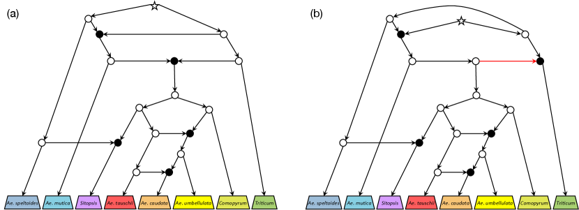
Fig. 8(a) shows a part of the biologically estimated tree-child network representing the evolutionary history of eight wheat relatives [18]. Note that the original network proposed in [18] is more complex, and we have ignored the uncertain reticulation arcs and selected some of the most likely reticulation arcs to create a tree-child network. Given the unrooted and undirected form of this network, Algorithm 2 successfully determined it as tree-child orientable. However, the algorithm could not recover the same network as in Fig. 8(a) and instead produced an alternative tree-child orientation with a different root position, such as the one shown in Fig. 8(b).
It is true that the networks differ in their deep ancestral reticulation histories due to the alternative root positions, but they agree with more recent important reticulation events explained in [18], namely the introgression of the Sitopsis ancestor by the Ae. speltoides ancestor and the complex gene flows from Ae. tauschii to Ae. caudata. Notably, despite the difference in the root position, most arc orientations remain consistent with the original network. This observation underscores the importance of allowing root flexibility to find desired orientations that might otherwise be overlooked.
While we have seen the similarity between the networks, the result also shows a significant limitation of the heuristic. Indeed, even for the root placement shown in Fig. 8(b), there exists a more accurate tree-child orientation that preserves the original reticulation structure, which can be obtained by reversing the red arc. The failure of Algorithm 2 to identify the better solution stems from its current objective function, which prioritises maximising the sum of distances between reticulations. This observation further highlights the challenge of developing biologically meaningful orientation heuristics.
8 Conclusion and future work
The -Orientation problem, which asks whether a given undirected binary phylogenetic network can be oriented to a directed phylogenetic network of a desired class , is an important computational problem in phylogenetics. The complexity of this problem remains unknown for many network classes , including the class of binary tree-child networks. A simple exponential time algorithm for -Orientation was provided in [1]. FPT algorithms for a special case of the problem were also proposed in [1], but their practical application is limited due to the intricate nature of the procedures and the challenges in implementation, despite the constraints imposed on . Additionally, no study has explored heuristic approaches to solve -Orientation in practice, even for a particular class such as tree-child networks.
In this paper, we have proposed a simple, easy to implement, practical exact FPT algorithm (Algorithm 1) for -Orientation and a heuristic algorithm for Tree-Child Orientation (Algorithm 2) based on Theorem 4. They improve the search space of the existing simple exponential time algorithm by using a cycle basis to reduce the number of possible reticulation placements. Our experiments showed that Algorithm 1 is significantly faster in practice than a state-of-the-art exponential time algorithm in [1]. Algorithm 2 is even faster, with a trade-off between the accuracy and the reticulation number. Further research using larger and more diverse datasets could provide more insight into the strengths and limitations of the proposed methods. Their usefulness and effectiveness should also be tested in real-world data analysis. As tree-child networks can describe evolutionary histories that do not involve frequent reticulation events, one can find various tree-child networks in the literature other than the one we used in Section 7.2, such as a hybridisation network of bread wheat (Fig. 3 in [19]), a hybridisation network of mosquitoes (Fig. 15 in [20]) and an admixture network of diverse populations (Fig. 3 in [21]).
Although we have used Tree-Child Orientation as a case study for performance evaluation, Algorithm 1 is applicable to orientation problems for classes other than tree-child networks. For example, orientation for stack-free networks [22] or tree-based networks [23] is expected to be a good application, because one can quickly decide whether a given network belongs to such a class. Speeding up Algorithm 1 and extending it to non-binary networks are topics for future research. It would be also interesting to consider alternative FPT algorithms that do not use a cycle basis.
Improving the accuracy of Algorithm 2 is also an interesting direction for future research. As discussed in Section 7, there are clearly rooms for improvement in the current objective function. Introducing a more suitable objective function may lead to the development of faster and more useful tree-child orientation heuristics.
Appendix A Algorithm for generating undirected binary phylogenetic networks
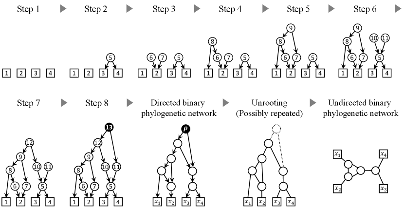
To create undirected binary phylogenetic networks on for the experiments, we used a simple method explained below (see Table 3 and Fig. 9 for illustrations). The code can be found at https://github.com/hayamizu-lab/tree-child-orienter/tree/main/Appendix. This method uses the idea of the coalescent model which is a popular approach for simulating phylogenetic trees.
Given a set of present-day species, we trace back lineages from the present to the past. At each step, lineages can either split with probability or coalesce with probability . If two lineages coalesce, a tree vertex is created, and the set of extant taxa is updated. If a lineage splits, a reticulation is created, and the set of extant taxa is updated. This process continues until all lineages coalesce into a single vertex, the root. The resulting graph becomes a rooted directed binary phylogenetic network on after the vertices of in-degree and out-degree are suppressed and the necessary vertex and arc are added to resolve the nonbinary vertices. It can then be converted to an undirected phylogenetic network on after suppressing the root and by ignoring all arc orientations and non-leaf vertex labels.
By adjusting the value of , we can generate phylogenetic networks with various reticulation numbers. When , no reticulations occur, and the generated networks are guaranteed to be phylogenetic trees. If has been set a larger value, the algorithm tends to produce graphs having more reticulations, as shown in Table 4. Thus, we generated undirected binary phylogenetic networks on with varying levels of complexity, and selected suitable ones in each computational experiment.
For Experiments 6.2 and 6.3, we generated various undirected binary phylogenetic networks on . The method requires the number of leaves and reticulation probability parameter to be specified. Table 4 summarises the breakdown of the generated graphs.
| Step | Taxon set | Selected lineage(s) | Event | New taxa | New arcs |
|---|---|---|---|---|---|
| 1 | 3,4 | Coalesce | 5 | ||
| 2 | 2 | Split | 6,7 | ||
| 3 | 1,6 | Coalesce | 8 | ||
| 4 | 7,8 | Coalesce | 9 | ||
| 5 | 5 | Split | 10,11 | ||
| 6 | 9,10 | Coalesce | 12 | ||
| 7 | 11,12 | Coalesce | 13 | ||
| 8 | - | - | - | - |
| Number of reticulations | ||||||||||||
| Total | ||||||||||||
| (10, 0.05) | 143 | 48 | 8 | 1 | 0 | 0 | 0 | 0 | 0 | 0 | 0 | 200 |
| (10, 0.1) | 99 | 67 | 20 | 9 | 3 | 2 | 0 | 0 | 0 | 0 | 0 | 200 |
| (10, 0.15) | 66 | 55 | 29 | 21 | 20 | 6 | 1 | 0 | 1 | 0 | 1 | 200 |
| (20, 0.05) | 73 | 82 | 31 | 10 | 3 | 0 | 0 | 0 | 1 | 0 | 0 | 200 |
| (20, 0.1) | 37 | 62 | 40 | 29 | 16 | 5 | 2 | 6 | 2 | 1 | 0 | 200 |
| (20, 0.15) | 14 | 19 | 37 | 38 | 30 | 18 | 18 | 10 | 7 | 4 | 5 | 200 |
| Total | 432 | 333 | 165 | 108 | 72 | 31 | 21 | 16 | 11 | 5 | 6 | 1200 |
Supplementary information The source code, datasets and detailed experimental results are available at https://github.com/hayamizu-lab/tree-child-orienter (archived at swh:1:dir:666a10c01c14741702fddd5f8704b30bc90299e5).
Acknowledgements We thank Yufeng Wu and Louxin Zhang for sharing code for randomly generating graphs, which we adapted for our experiments. We also appreciate the anonymous reviewers’ careful reading of our manuscript and useful comments.
Declarations
- Ethics approval and consent to participate
-
Not applicable.
- Consent for publication
-
Not applicable.
- Competing interests
-
The authors declare that they have no competing interests.
Funding MH is supported by JST FOREST Program Grant Number JPMJFR2135, Japan.
References
- \bibcommenthead
- Huber et al. [2024] Huber, K.T., Iersel, L., Janssen, R., Jones, M., Moulton, V., Murakami, Y., Semple, C.: Orienting undirected phylogenetic networks. Journal of Computer and System Sciences 140, 103480 (2024)
- Maeda et al. [2023] Maeda, S., Kaneko, Y., Muramatsu, H., Murakami, Y., Hayamizu, M.: Orienting undirected phylogenetic networks to tree-child network. arXiv preprint arXiv:2305.10162 (2023)
- Bulteau et al. [2023] Bulteau, L., Weller, M., Zhang, L.: On Turning A Graph Into A Phylogenetic Network. working paper or preprint (2023). https://hal.science/hal-04085424
- Cardona et al. [2008] Cardona, G., Rosselló, F., Valiente, G.: Comparison of Tree-child Phylogenetic Networks. IEEE/ACM Transactions on Computational Biology and Bioinformatics 6(4), 552–569 (2008)
- Semple [2016] Semple, C.: Phylogenetic Networks with Every Embedded Phylogenetic Tree a Base Tree. Bulletin of Mathematical Biology 78(1), 132–137 (2016)
- Robbins [1939] Robbins, H.E.: A Theorem on Graphs, with an Application to a Problem of Traffic Control. The American Mathematical Monthly 46(5), 281–283 (1939)
- Döcker and Linz [2025] Döcker, J., Linz, S.: On the existence of funneled orientations for classes of rooted phylogenetic networks. Theoretical Computer Science 1023, 114908 (2025) https://doi.org/10.1016/j.tcs.2024.114908
- Bulteau and Zhang [2023] Bulteau, L., Zhang, L.: The tree-child network problem and the shortest common supersequences for permutations are NP-hard. arXiv preprint arXiv:2307.04335 (2023)
- McDiarmid et al. [2015] McDiarmid, C., Semple, C., Welsh, D.: Counting phylogenetic networks. Annals of Combinatorics 19, 205–224 (2015)
- Gross et al. [2003] Gross, J.L., Yallen, J., Zhang, P.: Handbook of Graph Theory. CRC press, Boca Raton (2003)
- Diestel [2017] Diestel, R.: Graph Theory, 5th Edition. Springer, Berlin (2017)
- Bondy and Murty [2008] Bondy, J.A., Murty, U.S.R.: Graph Theory. Springer, London (2008)
- Stepanets [1964] Stepanets, G.F.: Basis systems of vector cycles with extremal properties in graphs. Uspekhi Matematicheskikh Nauk 19(2), 171–175 (1964)
- Deo et al. [1982] Deo, N., Prabhu, G., Krishnamoorthy, M.S.: Algorithms for Generating Fundamental Cycles in a Graph. ACM Transactions on Mathematical Software 8(1), 26–201342 (1982) https://doi.org/10.1145/355984.355988
- Horton [1987] Horton, J.D.: A polynomial-time algorithm to find the shortest cycle basis of a graph. Society for Industrial and Applied Mathematics Journal on Computing 16(2), 358–366 (1987)
- Coelho de Pina [1995] Pina, J.: Applications of shortest path methods. Ph.D. thesis, University of Amsterdam (December 1995). https://hdl.handle.net/11245/1.118244
- Amaldi et al. [2010] Amaldi, E., Iuliano, C., Rizzi, R.: Efficient Deterministic Algorithms for Finding a Minimum Cycle Basis in Undirected Graphs. In: Integer Programming and Combinatorial Optimization: 14th International Conference, IPCO 2010, Lausanne, Switzerland, June 9-11, 2010. Proceedings 14, pp. 397–410 (2010). Springer
- Glémin et al. [2019] Glémin, S., Scornavacca, C., Dainat, J., Burgarella, C., Viader, V., Ardisson, M., Sarah, G., Santoni, S., David, J., Ranwez, V.: Pervasive hybridizations in the history of wheat relatives. Science Advances 5(5), 9188 (2019) https://doi.org/10.1126/sciadv.aav9188 https://www.science.org/doi/pdf/10.1126/sciadv.aav9188
- Marcussen et al. [2014] Marcussen, T., Sandve, S.R., Heier, L., et al.: Ancient hybridizations among the ancestral genomes of bread wheat. Science 345(6194), 1250092 (2014) https://doi.org/10.1126/science.1250092 https://www.science.org/doi/pdf/10.1126/science.1250092
- Willems et al. [2014] Willems, M., Tahiri, N., Makarenkov, V.: A new efficient algorithm for inferring explicit hybridization networks following the Neighbor-Joining principle. Journal of Bioinformatics and Computational Biology 12(05), 1450024 (2014)
- Mallick et al. [2016] Mallick, S., Li, H., Lipson, M., et al.: The Simons Genome Diversity Project: 300 genomes from 142 diverse populations. Nature 538, 201–206 (2016) https://doi.org/10.1038/nature18964
- Semple and Simpson [2018] Semple, C., Simpson, J.: When is a Phylogenetic Network Simply an Amalgamation of Two Trees? Bulletin of Mathematical Biology 80(9), 2338–2348 (2018)
- Francis and Steel [2015] Francis, A.R., Steel, M.: Which Phylogenetic Networks are Merely Trees with Additional Arcs? Systematic Biology 64(5), 768–777 (2015) https://doi.org/%****␣sn-article.bbl␣Line␣375␣****10.1093/sysbio/syv037