Oscillatory solutions at the continuum limit of Lorenz 96 systems

Di Qi^a and Jian-Guo Liu^b

Abstract

In this paper, we study the generation and propagation of oscillatory solutions observed in the widely used Lorenz 96 (L96) systems. First, period-two oscillations between adjacent grid points are found in the leading-order expansions of the discrete L96 system. The evolution of the envelope of period-two oscillations is described by a set of modulation equations with strictly hyperbolic structure. The modulation equations are found to be also subject to an additional reaction term dependent on the grid size, and the period-two oscillations will break down into fully chaotic dynamics when the oscillation amplitude grows large. Then, similar oscillation solutions are analyzed in the two-layer L96 model including multiscale coupling. Modulation equations for period-three oscillations are derived based on a weakly nonlinear analysis in the transition between oscillatory and nonoscillatory regions. Detailed numerical experiments are shown to confirm the analytical results.

^aDepartment of Mathematics, Purdue University, 150 North University Street, West Lafayette, IN 47907, USA

^bDepartment of Mathematics and Department of Physics, Duke University, Durham, NC 27708, USA

1 Introduction

The Lorenz 96 (L96) system is a simple and illustrative model designed by E. N. Lorenz in 1996 [14] to study various representative features observed in the atmosphere. The original L96 model is later generalized to a two-layer version [25, 2] to include multiscale interactions. Though the L96 equations are deterministic, they demonstrate intrinsically chaotic behaviors in direct numerical solutions that display large uncertainty and instability [20, 15]. It shows that the L96 models can produce many remarkable statistical and stochastic features [13, 19, 1] in common with the climate system while maintain a much cleaner mathematical setting. Furthermore, the L96 system has been widely used as a prototype model to test model reduction methods in uncertainty quantification and data assimilation [16, 17, 21, 22], and to analyze different aspects of multiscale stochastic behaviors in chaotic dynamics [4, 7, 3]. In general, such complex chaotic behaviors in discrete dynamical systems can be understood by properties of numerical schemes and the corresponding conservation properties [24]. However, there is still not a thorough study from this perspective in the context of L96 systems to our knowledge.

The chaotic behavior in the L96 solutions is found to be closely linked to the automatic generation of oscillating solutions happening at the grid scale, which can be compared to the discrete dispersive numerical schemes. Similar oscillating solutions on mesh scale after the formation of shocks are generally observed and systematically analyzed under various dispersive schemes [9, 8, 6]. In contrast to the strong convergence and stability of viscous solutions to smooth inviscid flows such as the detailed studies in [26, 12, 11], the oscillations generated in dispersive numerical schemes do not vanish and are maintained in finite amplitude, while the wavelength of the oscillations remains within the grid size. It is demonstrated from different numerical schemes on the Burgers-Hopf equation [5, 10] that the oscillations will persist in the weak convergence of the oscillatory approximations. Inspired by this observation in dispersive schemes, it is found that solutions of the L96 systems exhibit similar behaviors in its way to develop fully chaotic dynamics from smooth initial data.

In this paper, we study the well-known complex chaotic behaviors observed in the discrete one and two-layer L96 systems in analog to the oscillatory solutions in dispersive schemes. First, we treat the discrete inviscid L96 model as a finite difference approximation and study its continuum limit with small grid size as $h\rightarrow 0$ . It shows that the L96 system agrees with the solution of the Burgers-Hopf equation in its leading order, while the higher-order corrections make the important contribution to create the competing oscillatory features found in the discrete L96 solutions (Proposition 1 and 2). Based on typical observations from numerical simulations, we perform a detailed investigation about the development of oscillations at the discrete grid size from classical smooth solutions of the initial value problem. In particular, we find the existence of representative period-two oscillatory solutions [10] due to the local conservation laws maintained in the L96 schemes. Corresponding modulation equations that describe the evolution of an envelope of the period-two oscillations are derived to characterize the development and evolution of these typical oscillating solutions. The Strang-type analysis [23] can be applied to show the convergence of the L96 scheme (Theorem 5 and Corollary 7). Further, the breakdown of the period-two oscillations due to the strong effect of an additional reaction term indicates the generation of fully chaotic behavior in the solution. This provides a precise characterization for the route to chaotic solutions through the intermediate oscillating regions in the L96 models with a finite grid size $h$ .

As a further development, we seek a closer look near the transition region from non-oscillatory to oscillatory solutions. It shows that the solution may generate more complicated period-three structures. Using a weakly nonlinear asymptotic analysis, we derive the modulation equations that govern such period-three oscillation features and show the convergence of the discrete model to this typical period-three structure in leading order (Theorem 8). In particular, we demonstrate the multiscale performance in the two-layer L96 model, and show the potential period-three oscillation phenomena. It is found that the large-scale states create a contact discontinuity in the small-scale variable from the large-scale forcing, which induces the oscillatory solutions. Besides, all the analytical results are supported by detailed numerical simulations of the one-layer and two-layer L96 models with different initial conditions.

In the rest of the paper is organized as follows: we provide a general discussion on the L96 model and its leading-order asymptotic equations in Section 2. The creation of period-two oscillations and the corresponding modulation equations are then derived in Section 3. The large and small scale coupling mechanism in the two-layer L96 model is discussed in Section 4 where a typical period-three solution is derived. Finally, a summarizing discussion is given in Section 5.

2 Leading-order equations of the Lorenz 96 model

The standard L96 model is given by the spatially discrete system with uniform forcing $F$ and a linear damping

\frac{du_{j}}{dt}=\left(u_{j+1}-u_{j-2}\right)u_{j-1}-u_{j}+F,\;j=1,\cdots,J.

(2.1)

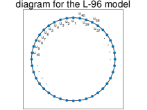
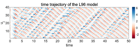
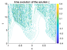
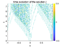
The model state variables $\mathbf{u}=\left(u_{1},u_{2},...,u_{J}\right)\in\mathbb{R}^{J}$ are defined with periodic boundary condition $u_{J+1}=u_{1}$ mimicking geophysical waves in the mid-latitude atmosphere. The discrete grid size is usually set to be $J=40$ denoting the non-dimensional midlatitude Rossby radius [1]. The model structure and a typical solution of (2.1) are illustrated in Figure 1. The discrete solution $\mathbf{u}$ is shown to demonstrate various representative chaotic dynamical features [13] such as westward (that is, moving to the left) wave packages and a rapid transition from regular initial state to highly chaotic solutions.

2.1 The L96 system as a finite difference discretization

In this paper, we focus on the nonlinear coupling term in the L96 system. If the forcing and damping terms in (2.1) are set to zero, we can rewrite the inviscid L96 model by introducing scaling parameters $a,h$ as

\frac{du_{j}}{dt}=\frac{1}{ah}\left(u_{j+1}-u_{j-2}\right)u_{j-1},

(2.2)

Above, the equation (2.2) is viewed as a semi-discrete difference scheme from a continuous function $u_{j}\left(t\right)=u\left(x_{j},t\right)$ with the spatial discretization $h=x_{j+1}-x_{j}=\frac{L}{J}$ where $J$ is the number of grid points and $L$ the domain size. For convenience in (2.2), we pick the difference factor $a=3$ . The inviscid L96 model builds an interesting bridge between the discrete L96 equation and the continuous Burgers-Hopf equation

\partial_{t}u-u\partial_{x}u=0.

(2.3)

It shows that they share very similar equilibrium statistical formalism through a detailed statistical performance analysis in [18, 1].

For a closer look at the link between the equations, we introduce the corresponding continuous state $u\left(x,t\right)$ defined on $\left[0,L\right]$ with periodic boundary condition $u\left(x\right)=u\left(x+L\right)$ . The continuum limit is reach as $h=\frac{L}{J}\rightarrow 0$ . By taking Taylor expansion as the finite difference approximation of $u\left(x_{j},t\right)$ with $x_{j}=jh$ directly, the continuum limit of the inviscid L96 system with $a=3$ yields

$\displaystyle\partial_{t}u=$	$\displaystyle u\partial_{x}u-\frac{h}{2}\left(u\partial_{xx}u+2\left(\partial_{x}u\right)^{2}\right)+\frac{h^{2}}{2}\left(u\partial_{xxx}u+2\partial_{x}u\partial_{xx}u\right)$	(2.4)
	$\displaystyle-\frac{h^{3}}{24}\left(5u\partial_{xxxx}u+16\partial_{x}u\partial_{xxx}u+6\left(\partial_{xx}u\right)^{2}\right)+O\left(h^{4}\right)$
$\displaystyle=$	$\displaystyle\frac{1}{2}\partial_{x}\left(u^{2}\right)-\frac{h}{2}\left(\partial_{xx}\left(u^{2}\right)-u\partial_{xx}u\right)+\frac{h^{2}}{6}\left(\partial_{xxx}\left(u^{2}\right)+u\partial_{xxx}u\right)$
	$\displaystyle-\frac{h^{3}}{24}\left(\partial_{xxxx}\left(u^{2}\right)+8\partial_{x}\left(u\partial_{xxx}u\right)-5u\partial_{xxxx}u\right)+O\left(h^{4}\right).$

From (2.4), it shows that the inviscid L96 model (2.2) can be viewed as a finite difference approximation to the Burgers-Hopf equation (2.3) in the leading order. Immediately, we find the two major conservation equations in the leading order

	$\displaystyle\frac{d}{dt}\int_{0}^{L}u\>dx=$	$\displaystyle-\frac{h}{2}\int_{0}^{L}\left(\partial_{x}u\right)^{2}dx+\frac{5h^{3}}{24}\int_{0}^{L}\left(\partial_{xx}u\right)^{2}dx+O\left(h^{4}\right),$		(2.5)
	$\displaystyle\frac{d}{dt}\int_{0}^{L}u^{2}dx=$	$\displaystyle\;O\left(h^{4}\right).$		(2.5)

The first equation in (2.5) shows that the spatially averaged mean state $\bar{u}=\int u\>dx$ is damped by $\int\left|\partial_{x}u\right|^{2}dx$ in the next order $O\left(h\right)$ . This implies the nonlinear coupling between the mean state and subscale modes. On the other hand, the total energy of the system, $E=\int u^{2}dx$ , is conserved up to the fourth order.

It is well-known that the initial value problem of the Burgers-Hopf equation (2.3) can create an infinite derivative in finite time due to the development of shocks. This process can be viewed as the ‘cascade of energy’ in turbulence from the mean state $\bar{u}=\int udx$ to multiscale fluctuation modes. To have a better understanding of the generation of chaotic behavior as shown in Figure 1, we need to dive into the next order approximation for the detailed nonlinear coupling between mean and fluctuation modes.

2.2 Conserved quantities in first-order approximation

Next, we discuss the additional effects induced from the first-order correction in the asymptotic approximation (2.4). When the solution $u$ of the continuum equation (2.4) remains $C^{2}$ , we can first identify the contribution from the first-order term $O\left(h\right)$ in the asymptotic expansion and focus on its leading order effect. This leads to the PDE

\partial_{t}u=u\partial_{xx}u-\partial_{xx}\left(u^{2}\right)=-u\partial_{xx}u-2\left(\partial_{x}u\right)^{2}.

(2.6)

Above in (2.6), we neglect the dependence on $h$ for the moment to focus on the individual contribution in this order. Similar to the conservation laws for the full equation (2.5), we can find the conserved energy and a dissipation on the momentum for the separate first-order equation (2.6)

	$\displaystyle\frac{d}{dt}\int udx$	$\displaystyle=-\int\left(\partial_{x}u\right)^{2}dx,$
	$\displaystyle\frac{d}{dt}\int u^{2}dx$	$\displaystyle=0.$

Based on the above conservation equations, we can introduce the decomposition for the model state $u\left(x,t\right)=\bar{u}\left(t\right)+u^{\prime}\left(x,t\right)$ into a spatial mean $\bar{u}$ and fluctuations $\int u^{\prime}dx=0$ with the following equations

\frac{d\bar{u}}{dt}=-\int\left(\partial_{x}u^{\prime}\right)^{2}dx,\quad\frac{d}{dt}\left(\bar{u}^{2}+\int u^{\prime 2}dx\right)=0.

(2.7)

The conservation equations (2.7) provide a crude illustration of the nonlinear coupling mechanism between the mean and fluctuations in the first level: the energy in the mean will be damped by the generation of oscillating fluctuation modes due to $u_{x}^{\prime}$ (developed from the leading-order Burgers-Hopf); and inversely the decrease in the mean energy will reinforce the energy in the fluctuation modes. This corresponds to the generation of oscillation solutions approximating the asymptotic equation (2.4), while the oscillating amplitude will not vanish as $h\rightarrow 0$ .

Furthermore, we can derive the conservation equation for any arbitrary function $G\left(u\right)$

\frac{d}{dt}\int G\left(u\right)dx=\int\left[G^{\prime\prime}\left(u\right)u-G^{\prime}\left(u\right)\right]\left(u_{x}\right)^{2}dx.

(2.8)

It can be checked that the above two conservation equations with $G\left(u\right)=u,u^{2}$ fit into the more general conservation equation (2.8). Further by setting $G\left(u\right)=\left|u\right|^{p}$ , we can find a sequence of conservation equations for any $p$

\frac{d}{dt}\int\left|u\right|^{p}dx=p\left(p-2\right)\int\mathrm{sign}\left(u\right)\left|u\right|^{p-1}\left(u_{x}\right)^{2}dx.

(2.9)

Using the above conservation equations, we are able to discover basic properties in the solutions of the first-order equation (2.6). First, it shows that the only stable steady state solution will be a constant with negative value. Further, we can show that the solutions of the equation (2.6) preserves negativity. More precisely, we summarize the results in the following propositions.

Proposition 1.

The only stable steady state solution of the equation (2.6) is the negative constant solution $u\equiv a<0$ .

Proof.

By letting $p=1$ in (2.9), we have

\frac{d}{dt}\int\left|u\right|dx=\int_{u<0}\left(u_{x}^{\prime}\right)^{2}dx-\int_{u>0}\left(u_{x}^{\prime}\right)^{2}dx.

(2.10)

In addition, assuming a steady state solution exist, the conditions in (2.7) requires

\frac{d\bar{u}}{dt}=0,\;\int\left(u_{x}^{\prime}\right)^{2}dx=0\;\Rightarrow\;u_{x}^{\prime}=0\;\Rightarrow u\equiv a=\mathrm{const.}

Next, consider any small mean-zero perturbations $u^{\prime}$ to the steady state solution $u=a+u^{\prime}$ . If the steady state satisfies $a<0$ so that $u=-\left|u\right|<0$ , we have $\bar{u}^{2}+\int u^{\prime 2}=C$ is conserved and $\bar{u}=-\int\left|u\right|$ increases in time according to (2.10). Thus the fluctuation $\int u^{\prime 2}$ will decrease to return to the constant steady state. On the other hand, if the steady state is $a>0$ , the conservation relation implies that $\bar{u}$ will decrease and the fluctuations $u^{\prime}$ will increase due to the equations for $\bar{u}$ and $\int\left|u\right|$ . Then the solution diverges from the original steady state. ∎

Proposition 2.

If the initial value of the equation (2.6) is fully negative, that is, $\max u_{0}\left(x\right)=b<0$ , the solution will remain negative for the entire time $t>0$

\max_{x}u\left(x,t\right)\leq b<0.

(2.11)

Proof.

Let

G\left(u\right)=\begin{cases}\left(u-b\right)^{2},&u\geq b,\\ 0,&u<b.\end{cases}

We have $G^{\prime\prime}u-G^{\prime}=2b$ when $u\geq b$ and $0$ otherwise. The conservation equation (2.8) gives that $\int G\left(u\right)$ is decreasing since

\frac{d}{dt}\int G\left(u\right)dx=2b\int_{u\geq b}\left(u_{x}\right)^{2}dx<0.

Together with the initial maximum value $b$ and the definition of the function $G$ , we find for all the time $t>0$

\int_{u\geq b}\left(u-b\right)^{2}dx=\int G\left(u\right)dx\leq\int G\left(u_{0}\right)dx=0\;\Rightarrow\;\int_{u\geq b}\left(u-b\right)^{2}dx\equiv 0.

This implies for all $t>0$ and almost everywhere in $x$

u\left(x,t\right)\leq b<0.

∎

On the other hand, there is no similar result for the positive solutions of (2.6). In fact from the proof in Proposition 2, a positive mean state $\bar{u}$ will excite more small-scale fluctuation modes. This will induce energy cascade to small scales in the transient state and drive the solution away from the positive initial state finally to the negative regime.

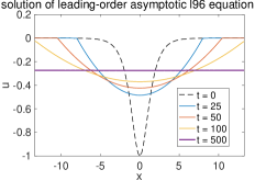
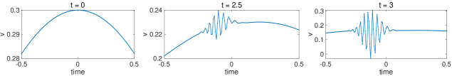
We check our analysis results above using direct numerical simulations of the equation (2.6). A pseudo-spectral scheme with dealiasing is used for high accuracy of the nonlinear coupling term [16]. We use a discretization size $J=256$ . Two different initial states with positive and negative initial values $u_{0}\left(x\right)=\pm\mathrm{sech}\left(x\right)$ are considered. First, Figure 2 shows the evolution of solution starting from a negative initial state. The solution remains in the smooth region and shows consistent performance as indicated in Proposition 1 and 2 as well as the energy conservation laws (2.7) and (2.9). Next, the solution development from positive initial state is displayed in Figure 3. In this case, we look at the transient state development from the unstable initial state. In contrast to the negative initial value case, the transient state of the solution demonstrates oscillations of period-two type (that is, oscillation between adjacent grid points). This implies the downward ‘cascade’ of energy to the smallest scale. Finally, the small-scale oscillations will be strongly dissipated, transferring to the final solution in the regime with purely negative values.

Remark.

The numerical examples in Figure 2 and 3 provide a first qualitative characterization of ‘the route to chaos’ in the L96 system. In the original setting of L96 model (2.1) with a positive forcing $F>0$ , the positive forcing will drive the mean state $\bar{u}$ to the positive value regime, while the first-order nonlinear coupling tend to create oscillatory solutions during returning to the stable regime with negative values. These competing counter effects lead to the creation of complex chaotic feature as shown in Figure 1.

3 Generation of period-two oscillatory solutions

Here, we study the development of oscillatory solutions in the discrete L96 model by considering its convergence at the continuum limit. As observed in the numerical simulation in Figure 3, period-two oscillating solutions in the grid size will automatically emerge from smooth initial data and be maintained from the leading-order nonlinear coupling effect. For the analysis, we treat the inviscid L96 system (2.2) as a spatially discretized numerical scheme in the following form

\frac{\partial u\left(x_{j},t\right)}{\partial t}=\frac{1}{ah}\left(u\left(x_{j+1},t\right)-u\left(x_{j-2},t\right)\right)u\left(x_{j-1},t\right).

(3.1)

Above, $a$ is a scaling parameter and $h=\frac{L}{J}$ is the spatial grid size. The continuous model state $u\left(x,t\right)$ defined on $x\in\left[0,L\right]$ is evaluated at the discretized grid points $x_{j}=jh$ with $j=1,\cdots,J$ such that $u\left(x,t\right)$ can be viewed as a smooth interpolation of the discrete grid values $u_{j}$ . In particular, the generalized scheme (3.1) goes back to the standard L96 equation (2.1) by taking the parameter values $a=3,J=40$ and $L=\frac{40}{3}$ .

3.1 Modulation equation with period-two oscillations

We start with two local conservation laws from the semi-discrete formulation (3.1)


$\displaystyle\frac{du_{j}^{2}}{dt}+\frac{1}{ah}\left(f_{j+\frac{1}{2}}-f_{j-\frac{1}{2}}\right)$	$\displaystyle=0,$	(3.2a)
$\displaystyle\frac{du_{j}}{dt}+\frac{1}{ah}\left(g_{j+\frac{1}{2}}-g_{j-\frac{1}{2}}\right)$	$\displaystyle=-\frac{h}{2a}D_{j+\frac{1}{2}}.$	(3.2b)

Above, we define the local fluxes for the energy $u_{j}^{2}$ and the momentum $u_{j}$

f_{j+\frac{1}{2}}=-2u_{j-1}u_{j}u_{j+1},\quad g_{j+\frac{1}{2}}=-\frac{1}{2}\left(u_{j-1}u_{j}+u_{j-1}u_{j+1}+u_{j}u_{j+1}\right),

(3.3)

and the additional non-conservative term for the momentum equation

D_{j+\frac{1}{2}}=\frac{u_{j+1}-u_{j-2}}{h}\frac{u_{j}-u_{j-1}}{h}.

(3.4)

Notice that the local conservation equations (3.2a) and (3.2b) is consistent with the asymptotic conservation equations (2.5) in Section 2.1. The energy $u_{j}^{2}$ accepts the exact conserved form locally, while the momentum $u_{j}$ is subject to an additional reaction term represented by the local differences in $D_{j+\frac{1}{2}}$ . As $h\rightarrow 0$ and $u$ remains a classical $C^{1}$ solution, the right hand side of (3.2b) goes to the higher-order limit, $-\frac{3h}{2a}\left(\partial_{x}u_{j}\right)^{2}$ . Thus the $C^{1}$ solution $u$ satisfies the exact conservation laws consistent with the classical solutions of the Burgers-Hopf equation before the formation of shocks. On the other hand, when the discontinuities are developed, it will be shown that the damping term $D_{j+\frac{1}{2}}$ on the right hand side will give an order one contribution due to the period-two oscillations.

To study the development of oscillations, we look at a special type of oscillating solutions developed from the conservation equations (3.2). We introduce the period-two states according to two adjacent grids

v_{j+\frac{1}{2}}=\frac{1}{2}\left(u_{j}+u_{j+1}\right),\quad w_{j+\frac{1}{2}}=\frac{1}{2}\left(u_{j}^{2}+u_{j+1}^{2}\right).

(3.5)

The above two averaged states correspond to the period-two oscillating solution referring to the alternating values between adjacent grid points, such at $u_{j}<u_{j-1}$ , $u_{j+1}>u_{j}$ , and $u_{j+2}<u_{j+1}$ . Thus, we are seeking the new smooth limiting states $w,v$ that satisfy the following period-two solution conditions

u_{j+1}=v_{j+\frac{1}{2}}+\left(-1\right)^{j}\left(w_{j+\frac{1}{2}}-v_{j+\frac{1}{2}}^{2}\right)^{\frac{1}{2}},\quad M_{j+\frac{1}{2}}=\left(w_{j+\frac{1}{2}}-v_{j+\frac{1}{2}}^{2}\right)^{\frac{1}{2}}=\frac{\left(-1\right)^{j}}{2}\left(u_{j+1}-u_{j}\right).

We can find the dynamical equations for the new period-two variables $\left(w_{j+\frac{1}{2}},v_{j+\frac{1}{2}}\right)$ by adding up the locally conserved equations (3.2a) and (3.2b) at two adjacent grid points, that is,


$\displaystyle\frac{dw_{j+\frac{1}{2}}}{dt}+\frac{1}{2ah}\left(f_{j+\frac{3}{2}}-f_{j-\frac{1}{2}}\right)$	$\displaystyle=0,$	(3.6a)
$\displaystyle\frac{dv_{j+\frac{1}{2}}}{dt}+\frac{1}{2ah}\left(g_{j+\frac{3}{2}}-g_{j-\frac{1}{2}}\right)$	$\displaystyle=-\frac{h}{4a}\left(D_{j+\frac{3}{2}}+D_{j+\frac{1}{2}}\right).$	(3.6b)

To first gain some intuition on the solutions of the above equations, we check the steady state period-two solution, $w_{j+\frac{1}{2}}\equiv\bar{w}$ , $v_{j+\frac{1}{2}}\equiv\bar{v}$ , and $\cdots=u_{j}=u_{j+2}=\cdots<$ $\cdots u_{j+1}=u_{j+3}=\cdots$ thus $M_{j+\frac{1}{2}}=u_{j+1}-u_{j}\equiv\bar{M}$ . This leads to the dynamical equations

\ \frac{d\bar{v}}{dt}=\frac{1}{2ah}\bar{M}^{2}>0,\quad\mathrm{and}\quad\frac{d\bar{w}}{dt}=0.

This implies how the solution performs when the period-two solution is developed. The mean energy state $\bar{w}=2\bar{v}^{2}+\frac{1}{2}\bar{M}^{2}$ will stay as a constant while the mean amplitude of $\bar{v}$ will increase when period-two oscillation is gradually generated in $u$ . This implies that the jump amplitude $\bar{M}$ will decrease in time, leading to a non-oscillating solution at the final steady state.

Next, to achieve a more precise characterization for the time evolution of the period-two oscillating solutions when discontinuity is developed in $u$ , we derive the modulation equations according to the above semi-discrete conservation equations (3.2). The flux terms can be expanded by Taylor series when $w,v$ are $C^{2}$ functions, that is,

	$\displaystyle-\frac{1}{2ah}\left(f_{j+\frac{3}{2}}-f_{j-\frac{1}{2}}\right)$	$\displaystyle=\frac{2}{a}\partial_{x}\left(2v^{2}-w\right)\left(v-\left(w-v^{2}\right)^{\frac{1}{2}}\right)\left(x_{j+\frac{1}{2}}\right)+O\left(h\right),$
	$\displaystyle-\frac{1}{2ah}\left(g_{j+\frac{3}{2}}-g_{j-\frac{1}{2}}\right)$	$\displaystyle=\frac{1}{2a}\partial_{x}\left(4v^{2}-w-2v\left(w-v^{2}\right)^{\frac{1}{2}}\right)\left(x_{j+\frac{1}{2}}\right)+O\left(h\right).$

And the difference term on the right hand side gives

-\frac{h}{4a}\left(D_{j+\frac{3}{2}}+D_{j+\frac{1}{2}}\right)=-\frac{2}{a}\partial_{x}\left(w-v^{2}\right)\left(x_{j+\frac{1}{2}}\right)+\frac{2}{a}\frac{M_{j+\frac{1}{2}}^{2}}{h}+O\left(h\right),

with $M_{j+\frac{1}{2}}^{2}=\frac{1}{4}\left(u_{j+1}-u_{j}\right)^{2}=w_{j+\frac{1}{2}}-v_{j+\frac{1}{2}}^{2}\geq 0$ . Notice that when the solution $u\left(x,t\right)$ is $C^{1}$ , $M_{j+\frac{1}{2}}^{2}\sim\left(\partial_{x}u\right)^{2}h^{2}$ , thus the last terms on the right hand side are of the next order $O\left(h\right)$ and vanish as $h\rightarrow 0$ . We have the following lemma in the region of classical solutions of $u$ .

Lemma 3.

The solution $\left(v,w\right)$ of the modulation state is $C^{1}$ before the formation of shock in $u$ of (3.1). And its leading-order equation as $h\rightarrow 0$ satisfies the following conservation form

	$\displaystyle\partial_{t}w$	$\displaystyle=\frac{2}{a}\partial_{x}\left(2v^{3}-vw\right),$		(3.7)
	$\displaystyle\partial_{t}v$	$\displaystyle=\frac{1}{a}\partial_{x}\left(2v^{2}-\frac{w}{2}\right),$		(3.7)

where we have $u=v\pm\left(w-v^{2}\right)^{\frac{1}{2}}$ .

However, when the period-two oscillation is developed after the formation of the shock, then we have $M_{j+\frac{1}{2}}^{2}\sim O\left(h\right)$ . This leads to the amplification of the period-two oscillations. In this case, we find the modulation equations describing the $C^{2}$ solutions $\left(w,v\right)$ with the existence of the period-two oscillations in $u$ at the continuum limit as $h\rightarrow 0$


$\displaystyle\partial_{t}w$	$\displaystyle=\frac{2}{a}\partial_{x}\left[2v^{3}-vw-\left(2v^{2}-w\right)\left(w-v^{2}\right)^{\frac{1}{2}}\right],$	(3.8a)
$\displaystyle\partial_{t}v$	$\displaystyle=\frac{1}{a}\partial_{x}\left[4v^{2}-\frac{5w}{2}-v\left(w-v^{2}\right)^{\frac{1}{2}}\right]+\frac{S}{2a},$	(3.8b)

where we define the smooth function $S\left(x,t\right)=\lim_{h\rightarrow 0}\frac{\left|u_{j+1}-u_{j}\right|^{2}}{h}$ as the additional reaction term due to the period-two oscillating solution. One first constraint for the smoothly varying states $\left(w,v\right)$ is $w\geq v^{2}$ from the definition. Above, the solution will remain smooth when $M_{j+\frac{1}{2}}$ grows to the order $O\left(\sqrt{h}\right)$ for large amplitude period-two oscillations in $u$ solutions. We can summarize the modulation equations (3.8) in the following lemma.

Lemma 4.

The leading-order equation of the semi-discretized scheme (3.1) as $h\rightarrow 0$ can be written according to the states $\mathbf{u}=\left(v,w\right)^{T}$ as

\partial_{t}\mathbf{u}-\partial_{x}\mathbf{F}=\mathbf{S},

(3.9)

with

\mathbf{F}=\left(f,g\right)^{T}=\frac{1}{a}\left(4v^{2}-\frac{5w}{2}-v\left(w-v^{2}\right)^{\frac{1}{2}},4v^{3}-2vw-2\left(2v^{2}-w\right)\left(w-v^{2}\right)^{\frac{1}{2}}\right)^{T}.

(3.10)

The additional reaction term $\mathbf{S}$ on the right hand side satisfies:

•

In the classical region with $u\in C^{1}$ , there is no additional source term on the right hand side $\mathbf{S=0}$ ;
•

In the period-two region where amplified oscillations are developed, that is, $\left|u_{j+1}-u_{j}\right|\sim O\left(\sqrt{h}\right)$ , we have the non-zero reaction term defined as $\mathbf{S}=\frac{1}{2a}\left(\lim_{h\rightarrow 0}\frac{\left|u_{j+1}-u_{j}\right|^{2}}{h},0\right)^{T}$ .

Remark.

1. The system (3.9) is called strictly hyperbolic if the Jacobian matrix

\nabla\mathbf{F}=\begin{bmatrix}\partial_{v}f&\partial_{w}f\\ \partial_{v}g&\partial_{w}g\end{bmatrix}=L^{-1}\Lambda L,

(3.11)

is diagonalizable and has real and separated eigenvalues.

2. The additional reaction term $S$ in (3.8b) comes from the discrete term $\frac{1}{h}M_{j+\frac{1}{2}}^{2}=\frac{1}{4h}\left(u_{j+1}-u_{j}\right)^{2}$ . This term will give a dominant contribution when the amplitude of period-two oscillation $\left|u_{j+1}-u_{j}\right|$ grows large. Still, (3.8) remains a good approximation to the discrete solution with a finite grid size $h$ .

3.2 Convergence to the period-two modulation equations

Here, we show the convergence of the discrete solution $\left(v_{j+\frac{1}{2}}\left(t\right),w_{j+\frac{1}{2}}\left(t\right)\right)$ in (3.5) to the smooth period-two solution $\left(v\left(x_{j+\frac{1}{2}},t\right),w\left(x_{j+\frac{1}{2}},t\right)\right)$ of the modulation equations (3.8) at the continuum limit as $h\rightarrow 0$ .

3.2.1 Convergence with small oscillation amplitude

First, we show that the modulation equation for $\left(v,w\right)$ gives a good approximation to the discrete period-two solution at the small oscillation amplitude case, $\left|u_{j+1}-u_{j}\right|=O\left(\sqrt{h}\right)$ . The theorem basically follows [10] according to the modulation equations (3.8).

Theorem 5.

Let $\mathbf{u}\left(x,t\right)=\left(v\left(x,t\right),w\left(x,t\right)\right)$ be a $C^{2}$ solution of the modulation equation (3.8), and $\mathbf{U}_{j+\frac{1}{2}}=\left(v_{j+\frac{1}{2}}\left(t\right),w_{j+\frac{1}{2}}\left(t\right)\right),j=1,\cdots,J$ be the discrete period-two solution from the inviscid L96 equation (3.1). If both solutions belong to the hyperbolic region (3.11) and $M_{j+\frac{1}{2}}^{2}=w_{j+\frac{1}{2}}-v_{j+\frac{1}{2}}^{2}=O\left(h\right)$ during the time interval $t\in\left[0,T\right]$ , we have

\max_{0\leq t\leq T}\left[\frac{1}{J}\sum_{j=1}^{J}\left|\mathbf{u}\left(x_{j+\frac{1}{2}},t\right)-\mathbf{U}_{j+\frac{1}{2}}\left(t\right)\right|^{2}\right]^{\frac{1}{2}}\leq C_{T}\frac{1}{J},

(3.12)

where $x_{j+\frac{1}{2}}=\left(j+\frac{1}{2}\right)h$ , $h=\frac{L}{J}$ , and $\left|\cdot\right|$ is the vector $L^{2}$ -norm.

Proof.

The $C^{2}$ solution $\mathbf{u}\left(x,t\right)$ of the modulation equation (3.8) can be summarized in the following equation as

\frac{d\mathbf{u}\left(x_{j+\frac{1}{2}},t\right)}{dt}=\frac{\mathbf{F}\left(\mathbf{u}\left(x_{j+\frac{3}{2}},t\right)\right)-\mathbf{F}\left(\mathbf{u}\left(x_{j-\frac{1}{2}},t\right)\right)}{2h}+\mathbf{S}\left(\mathbf{u}\left(x_{j+\frac{1}{2}},t\right)\right)+O\left(h\right).

Correspondingly, the solution $\mathbf{U}_{j+\frac{1}{2}}\left(t\right)$ of the discrete equations (3.6) can be rewritten as

\frac{d\mathbf{U}_{j+\frac{1}{2}}}{dt}=\frac{\mathbf{F}\left(\mathbf{U}_{j+\frac{3}{2}}\right)-\mathbf{F}\left(\mathbf{U}_{j-\frac{1}{2}}\right)}{2h}+\mathbf{S}\left(\mathbf{U}_{j+\frac{1}{2}}\right)+O\left(h\right).

In addition, Taylor expansions from the previous computations show that

\mathbf{F}\left(\mathbf{u}\left(x_{j+\frac{1}{2}},t\right)\right)-\mathbf{F}\left(\mathbf{U}_{j+\frac{1}{2}}\right)=\nabla\mathbf{F}_{j+\frac{1}{2}}\mathbf{e}_{j+\frac{1}{2}}+O\left(h\right),

where we introduce the error $\mathbf{e}_{j+\frac{1}{2}}\left(t\right)=\mathbf{u}\left(x_{j+\frac{1}{2}},t\right)-\mathbf{U}_{j+\frac{1}{2}}\left(t\right)$ and $\nabla\mathbf{F}_{j+\frac{1}{2}}=\nabla_{\mathbf{u}}\mathbf{F}\left(\mathbf{u}\left(x_{j+\frac{1}{2}},t\right)\right)$ is the gradient about $\mathbf{u}=\left(v,w\right)$ . Combining the above equations, we have

\frac{d\mathbf{e}_{j+\frac{1}{2}}}{dt}=\frac{\nabla\mathbf{F}_{j+\frac{3}{2}}\mathbf{e}_{j+\frac{3}{2}}-\nabla\mathbf{F}_{j-\frac{1}{2}}\mathbf{e}_{j-\frac{1}{2}}}{2h}+\nabla\mathbf{S}_{j+\frac{1}{2}}\mathbf{e}_{j+\frac{1}{2}}+O\left(h\right).

Hyperbolicity of the equations guarantees the eigenvalue decomposition of the coefficient matrix with real eigenvalues

\nabla\mathbf{F}_{j+\frac{1}{2}}=L_{j+\frac{1}{2}}^{-1}\Lambda_{j+\frac{1}{2}}L_{j+\frac{1}{2}}.

Therefore, by introducing $\mathbf{\tilde{e}}_{j+\frac{1}{2}}=L_{j+\frac{1}{2}}\mathbf{e}_{j+\frac{1}{2}}$ we have the dynamics for the error

	$\displaystyle\frac{d\mathbf{\tilde{e}}_{j+\frac{1}{2}}}{dt}-\frac{\Lambda_{j+\frac{3}{2}}\mathbf{\tilde{e}}_{j+\frac{3}{2}}-\Lambda_{j-\frac{1}{2}}\mathbf{\tilde{e}}_{j-\frac{1}{2}}}{2h}=$	$\displaystyle L_{j+\frac{1}{2}}^{-1}\left(\frac{L_{j+\frac{3}{2}}-L_{j+\frac{1}{2}}}{2h}\Lambda_{j+\frac{3}{2}}\mathbf{\tilde{e}}_{j+\frac{3}{2}}+\frac{L_{j+\frac{1}{2}}-L_{j-\frac{1}{2}}}{2h}\Lambda_{j-\frac{1}{2}}\mathbf{\tilde{e}}_{j-\frac{1}{2}}\right)$
		$\displaystyle+\frac{dL_{j+\frac{1}{2}}}{dt}L_{j+\frac{1}{2}}^{-1}\mathbf{\tilde{e}}_{j+\frac{1}{2}}+L_{j+\frac{1}{2}}\nabla\mathbf{S}_{j+\frac{1}{2}}L_{j+\frac{1}{2}}^{-1}\mathbf{\tilde{e}}_{j+\frac{1}{2}}+O\left(h\right)$
	$\displaystyle\leq$	$\displaystyle C\left(\left\|\mathbf{\tilde{e}}_{j-\frac{1}{2}}\right\|+\left\|\mathbf{\tilde{e}}_{j+\frac{1}{2}}\right\|+\left\|\mathbf{\tilde{e}}_{j+\frac{3}{2}}\right\|\right)+C_{1}h.$

Multiplying both sides by $\tilde{\mathbf{e}}_{j+\frac{1}{2}}$ and taking the summation about $j$ gives using the smooth dependence on $\mathbf{u}$

\frac{d}{dt}\frac{1}{2}\sum_{j}\left|\mathbf{\tilde{e}}_{j+\frac{1}{2}}\right|^{2}-\sum_{j}\frac{\Lambda_{j+\frac{1}{2}}-\Lambda_{j-\frac{1}{2}}}{2h}\mathbf{\tilde{e}}_{j-\frac{1}{2}}\cdot\mathbf{\tilde{e}}_{j+\frac{1}{2}}\leq\sum_{j}\left[C\left|\tilde{\mathbf{e}}_{j+\frac{1}{2}}\right|\left(\left|\mathbf{\tilde{e}}_{j-\frac{1}{2}}\right|+\left|\mathbf{\tilde{e}}_{j+\frac{1}{2}}\right|+\left|\mathbf{\tilde{e}}_{j+\frac{3}{2}}\right|\right)+C_{1}\left|\tilde{\mathbf{e}}_{j+\frac{1}{2}}\right|h\right].

This leads to the estimate for the total error

	$\displaystyle\frac{d}{dt}\sum_{j}\left\|\mathbf{\tilde{e}}_{j+\frac{1}{2}}\right\|^{2}$	$\displaystyle\leq C\sum_{j}\left\|\mathbf{\tilde{e}}_{j+\frac{1}{2}}\right\|^{2}+hC_{1}\sum_{j}\left\|\mathbf{\tilde{e}}_{j+\frac{1}{2}}\right\|$
		$\displaystyle\leq C^{\prime}\sum_{j}\left\|\mathbf{\tilde{e}}_{j+\frac{1}{2}}\right\|^{2}+C_{1}^{\prime}h.$

Using Gronwall’s inequality for any $t\leq T$ , we have

\sum_{j}\left|\mathbf{\tilde{e}}_{j+\frac{1}{2}}\right|^{2}\left(t\right)\leq C_{T}h\;\Rightarrow\;\frac{1}{J}\sum_{j}\left|\mathbf{e}_{j+\frac{1}{2}}\right|^{2}\left(t\right)\leq C_{T}h^{2}.

This establishes the final result in the theorem with $C_{T}$ independent of $h$ . ∎

Remark.

In Theorem 5, we require small oscillation amplitude $M_{j+\frac{1}{2}}\sim\left|u_{j+1}-u_{j}\right|=O\left(\sqrt{h}\right)$ in the period-two solution while its derivative blows up $\frac{u_{j+1}-u_{j}}{h}=O\left(1/\sqrt{h}\right)$ . When the oscillations grow to larger amplitude $M_{j+\frac{1}{2}}^{2}=\frac{1}{2}\left|u_{j+1}-u_{j}\right|^{2}=O\left(1\right)$ , the unbounded $S=\frac{M^{2}}{h}$ will take over as the dominant term and break down the period-two oscillations. Still, according to the equation for $M$ shown next in (3.13), the time scale of the oscillation amplitude $M$ is within $T\sim O\left(h\right)$ . We still have a bounded estimation in the error $\sum_{j}\left|\mathbf{e}_{j+\frac{1}{2}}\right|^{2}\leq\frac{C}{J}e^{TJ}\sim\frac{C^{\prime}}{J}$ , thus the solution of the modulation equation (3.8) can still offer a desirable estimation to the discrete period-two solution of (3.1) with a moderate grid size $h$ (which is in fact the case of the standard L96 model using $J=\frac{1}{h}=40$ ).

3.2.2 Approximation with large oscillation amplitude

Next, we can check the development of large period-two oscillations by introducing an additional equation for $M=\left(w-v^{2}\right)^{\frac{1}{2}}$ . When strong oscillations are induced, we assume $M_{j+\frac{1}{2}}=\frac{\left(-1\right)^{j}}{2}\left(u_{j+1}-u_{j}\right)$ describing the jump amplitude between two adjacent grids. The dynamical equation for the difference can be written down as

\frac{dM_{j+\frac{1}{2}}}{dt}=\frac{\left(-1\right)^{j}}{2ah}\left[\left(u_{j+2}-u_{j-1}\right)u_{j}-\left(u_{j+1}-u_{j-2}\right)u_{j-1}\right].

Through Taylor expansion of the difference form up to $O\left(h\right)$ , the continuum equation is reached as

\partial_{t}M=-\frac{2}{ah}vM-\frac{1}{2a}\partial_{x}\left(M^{2}-v^{2}+w\right).

(3.13)

The first term $-\frac{2v}{ah}M$ on the right hand side of (3.13) shows that the period-two oscillation will be amplified in the domain where $v<0$ , while the oscillations will be damped where $v>0$ . In addition, the advection term implies that the period-two oscillations will propagate with velocity $v$ . Especially, combining with (3.8), we can rewrite the closed system for $\left(v,M\right)$ with finite oscillation amplitude

	$\displaystyle\partial_{t}v$	$\displaystyle=\frac{2M^{2}}{ah}+\frac{1}{a}\partial_{x}\left(\frac{3}{2}v^{2}+\frac{5}{2}M^{2}-vM\right),$		(3.14)
	$\displaystyle\partial_{t}M$	$\displaystyle=-\frac{2v}{ah}M-\frac{1}{a}\partial_{x}M.$		(3.14)

Above, we assume $M\sim O\left(1\right)$ grows to an order one term, and the equations for $v$ and $M$ have the stiff leading order term dependent on the grid size $h^{-1}$ .

Then, we can separate the leading-order term and investigate its effect on the particular solution $\left(v_{h},M_{h}\right)$

\partial_{t}v_{h}=\frac{2M_{h}^{2}}{ah},\quad\partial_{t}M_{h}=-\frac{2v_{h}}{ah}M_{h}.

(3.15)

Directly integrating the above equation leads to the following lemma about a closed form of the solution of (3.15).

Lemma 6.

The leading-order equations (3.15) for $\left(v_{h},M_{h}\right)$ have the explicitly integrable solution

v_{h}\left(x,t\right)=\lambda\left(x\right)\frac{1-\mu\left(x\right)\exp\left(-\frac{4\lambda}{ah}t\right)}{1+\mu\left(x\right)\exp\left(-\frac{4\lambda}{ah}t\right)},\quad M_{h}\left(x,t\right)=\frac{2\lambda\left(x\right)\sqrt{\mu\left(x\right)}}{1+\mu\left(x\right)\exp\left(-\frac{4\lambda}{ah}t\right)}\exp\left(-\frac{2\lambda}{ah}t\right),

(3.16)

where $\lambda,\mu\geq 0$ are smooth functions determined by the initial values of $v_{h},M_{h}$ . Further in the full equations (3.14), if $v=v_{h}+O\left(h\right)$ , there is also $M=M_{h}+O\left(h\right)$ .

Proof.

Equations (3.15) are actually a coupled ODE system and satisfy

\partial_{t}^{2}v=-\frac{2}{ah}\partial_{t}v^{2}\;\Rightarrow\;\partial_{t}v=-\frac{2}{ah}v^{2}+C\left(x\right).

The constant can be found from the initial value $C=\partial_{t}v\left(x,0\right)+\frac{2}{ah}v^{2}\left(x,0\right)>0$ , with a small enough $h$ . For convenience, we introduce $C=\frac{2\lambda^{2}}{ah}$ . Therefore, by integrating the above equation again about $v$ and $t$ , we find

\left|\frac{\lambda+v}{\lambda-v}\right|=\left|\frac{\lambda+v_{0}}{\lambda-v_{0}}\right|e^{\frac{2}{ah}t}=\mu^{-1}e^{\frac{4\lambda}{ah}t}\;\Rightarrow\;v=\lambda\frac{1-\mu e^{-\frac{4\lambda}{ah}t}}{1+\mu e^{-\frac{4\lambda}{ah}t}}.

And the expression for $M$ follows immediately from the above solution of $v$ .

Next, let $v=v_{h}+\tilde{v}h$ and $M=M_{h}+\tilde{M}h$ . In the equation for $M$ in (3.14), the last advection term can be canceled by changing $M\left(x,t\right)\rightarrow M\left(x+\frac{1}{a}t,t\right)$ . Thus, the equation satisfies using the solution (3.15)

\partial_{t}\tilde{M}=-\frac{2}{ah}\left(v_{h}+\tilde{v}h\right)\tilde{M}-\frac{2}{ah}M_{h}\tilde{v}.

Integrating the equation in time, we get

	$\displaystyle\left\|\tilde{M}\left(t\right)\right\|$	$\displaystyle\leq\frac{2}{ah}\int_{0}^{t}e^{-\frac{2}{ah}\int_{s}^{t}\left(v_{h}\left(\tau\right)+\tilde{v}\left(\tau\right)h\right)d\tau}M_{h}\left(s\right)\left\|\tilde{v}\left(s\right)\right\|ds$
		$\displaystyle\leq\frac{2}{ah}\int_{0}^{t}e^{\frac{\lambda}{ah}s+C}M_{h}\left(s\right)\left\|\tilde{v}\left(s\right)\right\|ds$
		$\displaystyle\leq\frac{C}{h}\int_{0}^{t}\exp\left(-\frac{\lambda}{ah}s\right)ds\leq C^{\prime}.$

Above, the second line uses the explicit solution of $v_{h}$ , $\left|\int_{s}^{t}v_{h}\left(\tau\right)d\tau\right|\leq\frac{\lambda}{2}s+C_{1}h$ , and the uniform boundedness of $\tilde{v}$ , $\left|\int_{s}^{t}\tilde{v}\left(\tau\right)hd\tau\right|\leq C_{2}h$ . And the third line again uses the explicit solution of $M_{h}$ and uniform bound of $\tilde{v}$ . Thus we show $\tilde{M}$ is also uniformly bounded from $h$ . ∎

Lemma 6 provides a more precise estimate for the development of oscillation amplitude $M$ dependent on the grid size $h$ . This implies that the leading-order equation gives the uniformly bounded solution $v_{h}$ and the uniformly decaying solution $M_{h}$ independent of the stiff factor $h^{-1}$ . According to this leading-order performance, we can introduce the new modulation equations for $\left(v,w\right)$ dependent on finite grid size $h$

	$\displaystyle\partial_{t}w$	$\displaystyle=\frac{2}{a}\partial_{x}\left[v\left(2v^{2}-w\right)-\left(2v^{2}-w\right)\left(w-v^{2}\right)^{\frac{1}{2}}\right],$		(3.17)
	$\displaystyle\partial_{t}v$	$\displaystyle=\frac{2\left(w-v^{2}\right)}{ah}+\frac{1}{a}\partial_{x}\left[4v^{2}-\frac{5w}{2}-v\left(w-v^{2}\right)^{\frac{1}{2}}\right].$		(3.17)

With this, we can generalize the result in Theorem 5 to the time with large period-two oscillation amplitude, $\left|u_{j+1}-u_{j}\right|=O\left(1\right)$ .

Corollary 7.

Let $\mathbf{u}=\left(v,w\right),t\in\left[0,T\right]$ be the $C^{2}$ solution of the modulation equation (3.17), and $\mathbf{U}_{j+\frac{1}{2}}=\left(v_{j+\frac{1}{2}},w_{j+\frac{1}{2}}\right),j=1,\cdots,J$ the discrete period-two solution from the inviscid L96 equation (3.1). Assume that $v$ and $w$ are both uniformly bounded for any $h>0$ and $v=v_{h}+O\left(h\right)$ for any $0\leq t\leq T$ , then we have

\max_{0\leq t\leq T}\left[\frac{1}{J}\sum_{j=1}^{J}\left|\mathbf{u}\left(x_{j+\frac{1}{2}},t\right)-\mathbf{U}_{j+\frac{1}{2}}\left(t\right)\right|^{2}\right]^{\frac{1}{2}}\leq C_{T}\frac{1}{J}.

(3.18)

Proof.

Notice that the only difference in the new modulation equations (3.17) is the new factor $\frac{1}{h}$ in the reaction equation. Thus the equation for the error $\mathbf{e}_{j+\frac{1}{2}}\left(t\right)=\mathbf{u}\left(x_{j+\frac{1}{2}},t\right)-\mathbf{U}_{j+\frac{1}{2}}\left(t\right)$ becomes

\frac{d\mathbf{e}_{j+\frac{1}{2}}}{dt}=\frac{1}{h}M_{j+\frac{1}{2}}\nabla\mathbf{M}_{j+\frac{1}{2}}\mathbf{e}_{j+\frac{1}{2}}+\frac{\nabla\mathbf{F}_{j+\frac{3}{2}}\mathbf{e}_{j+\frac{3}{2}}-\nabla\mathbf{F}_{j-\frac{1}{2}}\mathbf{e}_{j-\frac{1}{2}}}{2h}+O\left(h\right),

where $\mathbf{M}_{j+\frac{1}{2}}=\frac{2}{a}\left(M,0\right)^{T}\left(x_{j+\frac{1}{2}},t\right)$ and $M^{2}=w-v^{2}$ . Using the explicit leading-order solution $M_{h}$ and Lemma 6, we have $\left|M_{j+\frac{1}{2}}\right|\leq C\exp\left(-\frac{2\bar{\lambda}}{ah}t\right)+Ch$ and $\bar{\lambda}=\min_{j}\lambda_{j+\frac{1}{2}}$ . Following the same line of argument as in Theorem 5, we get the error estimate

\frac{d\mathbf{e}_{j+\frac{1}{2}}}{dt}\leq\left[C_{1}+\frac{C}{h}\exp\left(-\frac{2\bar{\lambda}}{ah}t\right)\right]\left(\left|\mathbf{e}_{j-\frac{1}{2}}\right|+\left|\mathbf{e}_{j+\frac{1}{2}}\right|+\left|\mathbf{e}_{j+\frac{3}{2}}\right|\right)+C_{2}h.

Finally, Gronwall’s inequality yields

\sum_{j}\left|\mathbf{e}_{j+\frac{1}{2}}\right|^{2}\left(t\right)\leq\left[C_{T}+\exp\left(\frac{C}{h}\int_{0}^{T}e^{-\frac{2\lambda}{ah}t}dt\right)\right]h\leq\left[C_{T}+\exp\left(\frac{a}{2\bar{\lambda}}\right)\right]h=C_{T}^{\prime}h.

∎

Remark.

It is found in the numerical simulations that it is usually the driven effect of the reaction term $\frac{M^{2}}{h}$ rather than the moving out of the hyperbolic region that breaks down the period-two oscillatory solutions. The leading $O\left(h^{-1}\right)$ terms combined with the additional $O\left(1\right)$ terms on the right hand sides of (3.14) may lead to complicated coupling dynamics, thus finally drive the solution away from the small perturbation region $v=v_{h}+O\left(h\right)$ required in the above theorem. Then, the clean period-two solution will break down to create fully chaotic features.

3.3 Persistence and breakdown of period-two oscillations

Now if we consider the leading flux term $\mathbf{F}$ in the modulation equation (3.10), the Jacobian matrix (3.11) becomes

\nabla\mathbf{F}=\frac{1}{a}\begin{bmatrix}8v-\left(w-v^{2}\right)^{\frac{1}{2}}+v^{2}\left(w-v^{2}\right)^{-\frac{1}{2}}&-\frac{5}{2}-\frac{1}{2}v\left(w-v^{2}\right)^{-\frac{1}{2}}\\ 12v^{2}-2w-8v\left(w-v^{2}\right)^{\frac{1}{2}}+2v\left(2v^{2}-w\right)\left(w-v^{2}\right)^{-\frac{1}{2}}&-2v+2\left(w-v^{2}\right)^{\frac{1}{2}}-\left(2v^{2}-w\right)\left(w-v^{2}\right)^{-\frac{1}{2}}\end{bmatrix}.

Solving the eigenvalues of the above matrix reveals that the condition for hyperbolicity of the modulation equation is always satisfied when $w-v^{2}>0$ , thus the solution always remains in the hyperbolic region. Still, if we consider the weakly oscillatory region up to order $O\left(\sqrt{h}\right)$ and neglect the higher-order terms due to $w-v^{2}=O\left(h\right)$ , the hyperbolic region with real eigenvalues requires

w^{2}>4v\left(3w-2v^{2}\right)\left(w-v^{2}\right)^{\frac{1}{2}}.

(3.19)

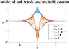
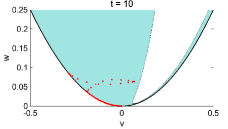
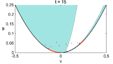
This gives the condition for maintaining only weakly period-two oscillations within $\left|u_{j+1}-u_{j}\right|=O\left(\sqrt{h}\right)$ . The hyperbolic region and the development of oscillatory solutions are illustrated in Figure 6. The period-two oscillations gradually developed large amplitudes and moved out of the weak oscillation hyperbolic region. This leads to a dominant reaction term $\frac{M^{2}}{h}$ that finally destroyed the period-two oscillation.

To see the breakdown of the period-two oscillations more clearly, it can be found directly from (3.13) that

\frac{1}{2}\partial_{t}M^{2}=-\frac{2v}{ah}M^{2}-\frac{1}{2a}\partial_{x}M^{2}\;\Rightarrow\;\frac{d}{dt}\frac{1}{2}\int_{\Omega}M^{2}dx=-\frac{2}{ah}\int_{\Omega}vM^{2}dx,

where the integration is taken in the oscillatory region $\Omega$ so that $M^{2}\mid_{\partial\Omega}=0$ . Thus a necessary condition of generating growing oscillation amplitude $M$ requires $v<0$ at some point of the domain. In addition, it implies that the period-two oscillation will emerge at an approximate growth rate of $\left|\frac{v}{h}\right|$ depending on the discrete grid size. As the amplitude of oscillations grows, $v$ will finally reach positive values at some point. Then, the periodic-two oscillation will starts to get damped at the points where $v$ reaches positive values. These features are explicitly observed in the numerical experiments in Figure 5 and are consistent with the leading-order solution (3.16).

In addition, we can check the instability in the semi-discrete system (3.1) around a steady mean state $\bar{u}$ . As in the previous section, introduce the mean-fluctuation decomposition of the state $u\left(x_{j},t\right)=\bar{u}+\tilde{u}_{j}\left(t\right)$ . The linearized equation of (3.1) becomes

\frac{d\tilde{u}_{j}}{dt}=\frac{1}{ah}\bar{u}\left(\tilde{u}_{j+1}-\tilde{u}_{j-2}\right).

Assuming the plane wave solution $\tilde{u}_{j}=e^{i\left(kx_{j}-\omega_{k}t\right)}$ , we find the dispersion relation

	$\displaystyle\omega_{k}$	$\displaystyle=\frac{\bar{u}}{ah}\left[-\left(\sin kh+\sin 2kh\right)+i\left(\cos kh-\cos 2kh\right)\right]$
		$\displaystyle=\frac{\bar{u}}{ah}\left[-\sin kh\left(1+2\cos kh\right)+i\left(-2\cos^{2}kh+\cos kh+1\right)\right].$

Positive growth rate for the fluctuation modes is induced if the imaginary part $\mathrm{Im}\omega_{k}>0$ . Thus we have that instability is induced when $\bar{u}>0,\cos kh>-\frac{1}{2}$ or $\bar{u}<0,\cos kh<-\frac{1}{2}$ . Especially, in the case when $\bar{u}<0$ , the maximum growth rate $c_{*}=\frac{-2\bar{u}}{ah}$ is reached at the critical wavenumber $k_{*}=\frac{\pi}{h}$ and we have $\mathrm{Re}\omega_{k_{*}}=0$ . The corresponding critical plane wave solution becomes

\tilde{u}_{j}^{*}=e^{i\left(k_{*}jh-\omega_{k_{*}}t\right)}=e^{\frac{-2\bar{u}}{ah}t}\left(-1\right)^{j}.

This implies that the period-two oscillation can be excited automatically from a negative mean velocity $\bar{u}<0$ . This is also confirmed in the numerical results in Figure 5 where the period-two oscillations are amplified in the region with $\bar{u}<0$ .

To summarize, we can describe the evolution of the solution of (3.1) in the following three stages, as the classical region, period-two region, and finally the fully chaotic region:

•

Stage I. Smooth state $u$ in the starting time: the state $u\left(x,t\right)$ remains as a $C^{2}$ function, so the solution performs as the Burgers-Hopf equation until the development of discontinuity;
•

Stage II. Development of period-two oscillation solution: small amplitude period-two oscillations are developed in $u$ at the point of discontinuity, while the modulation states $\left(v,w\right)$ stay as $C^{2}$ functions;
•

Stage III. Breakdown of period-two solution: Period-two oscillations increase to the positive region with $v>0$ and finally get damped. The states $\left(v,w\right)$ break down from the period-two oscillations, thus fully chaotic solution begins to develop.

3.4 Numerical verification for the development of oscillatory solutions

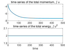
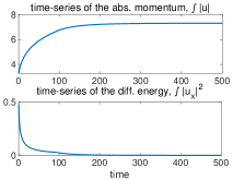
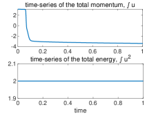
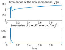
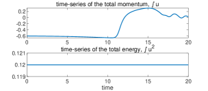
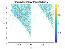
In the numerical experiments, we run the L96 model (3.1) with discretization $J=256$ and model parameters $a=3$ and $h=8/J$ . The initial state is taken as $u_{0}\left(x\right)=-0.3\mathrm{sech}^{2}\left(\frac{x}{2}\right)$ . We pick the negative initial value since the period-two solution can be induced from $\bar{u}<0$ from the linear instability. The 4th-order Runge-Kutta method is used for the time integration with time step $\Delta t=1\times 10^{-3}$ to achieve desirable accuracy. First, the time evolution of total momentum $\int udx$ and total energy $\int u^{2}dx$ as well as the related quantities are plotted in the upper panel of Figure 4. The solution starts with the classical solution with smooth $u$ . Consistent with our analysis in Section 2, the total energy is strictly conserved, while the total momentum is slowly decaying due to the damping from $-\int u_{x}^{2}dx$ . $\int\left|u\right|dx$ is also increasing in the classical region since we have $u<0$ in the initial time.

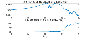
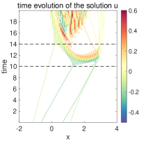
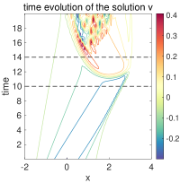
Next, a shock is developed in $u$ at around $t=10$ . This leads to the oscillations in $u$ and the creation of period-two solution. This can be observed in the lower panel of Figure 4 for the time evolutions of $u$ and $v,w$ and more clearly in the several time snapshots of $u,v,w$ in Figure 5. Especially, we observe that $v$ starts to increase in this region due to the reaction term $S>0$ in the equation for of $v$ . Period-two oscillations at the grid size are automatically developed at the left side of the discontinuity and quickly get amplified. At the same time, the period-two solutions $v,w$ remain smooth except at the point of discontinuity.

Finally, $u$ evolves into positive values with the increasing oscillation amplitudes, and the period-two oscillations in the region with $v>0$ get damped. The smooth period-two solutions $v,w$ break down and fully chaotic behaviors of the solution start to emerge. This indicates the generation of many complex features as observed in the L96 system. We further show in Figure 6 the evolution of solutions $\left(v,w\right)$ beyond the hyperbolic region computed in (3.19). It shows that the oscillatory period-two solutions gradually develop in amplitude and evolve out to the fully chaotic behavior.

4 The two-layer Lorenz 96 system and period-three oscillations

As a further generalization of the original one-layer system, the two-layer L96 system [2, 25] introduces an additional second layer $v_{j,l}$ to each of the original L96 system state $u_{j},j=1,\cdots,J$ such that

	$\displaystyle\frac{du_{j}}{dt}$	$\displaystyle=\left(u_{j+1}-u_{j-2}\right)u_{j-1}-du_{j}+F-\frac{\tilde{h}\tilde{c}}{\tilde{b}}\sum_{s=1}^{L}v_{j,s}$		(4.1)
	$\displaystyle\frac{dv_{j,l}}{dt}$	$\displaystyle=-\tilde{c}\tilde{b}\left(v_{j,l+2}-v_{j,l-1}\right)v_{j,l+1}-\tilde{c}v_{j,l}+\frac{\tilde{h}\tilde{c}}{\tilde{b}}u_{j}.$		(4.1)

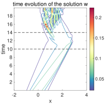
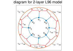
The new layer variables $v_{j,l}=v_{i}$ with $l=1,\cdots,L$ can be viewed as small scales with the ‘stretched’ reorganized index $i=l+L\left(j-1\right)$ . Periodic boundary conditions are used for both the two sets of variables, $u_{j+J}=u_{j}$ and $v_{i+JL}=v_{i}$ . In general, $u_{j}$ states are large-amplitude and low-frequency, each of which is coupled to a branch of the small-amplitude high-frequency variables $v_{j,l}$ . Notice that the second layer states $v_{j,l}$ in the two-layer L96 model above are only locally coupled with the corresponding first layer state $u_{j}$ . In the model parameters, $\tilde{h}$ is the coupling coefficient, $\tilde{b}$ is the spatial-scale ratio, and $\tilde{c}$ is the time-scale ratio. The large and small scale coupling structure is illustrated in Figure 7.

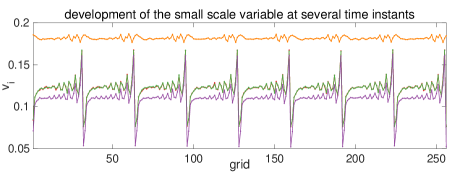
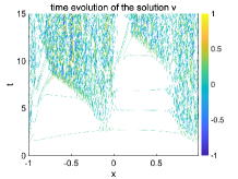
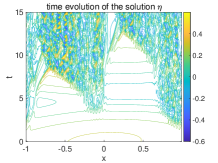
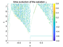
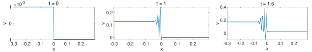
A typical solution of the small-scale state $v_{i}$ at several time instants is illustrated in Figure 7. It is observed that oscillatory solutions are generated at the boundaries of the large-scale state $u_{j}$ similar to that in the one-layer model. However, it also shows that the oscillations are no longer within the grid size, while in particular it appears that the period-three solution will emerge in this case due to the large and small scale coupling of states.

4.1 Strong scale separation with two interacting large-scale states

In analyzing oscillatory solutions of the two-layer L96 model as it approaches the continuous limit, we again focus on the nonlinear and multiscale coupling terms (that is, neglecting the forcing and damping effects in both large and small scales of (4.1)), and introduce the new parameters indicating the two different scales explicitly as

	$\displaystyle\frac{du\left(X_{j},t\right)}{dt}$	$\displaystyle=\left(u\left(X_{j+1},t\right)-u\left(X_{j-2},t\right)\right)u\left(X_{j-1},t\right)-h\sum_{l=1}^{L}v\left(X_{j},x_{l},t\right)$		(4.2)
	$\displaystyle\frac{dv\left(X_{j},x_{l},t\right)}{dt}$	$\displaystyle=-\frac{\gamma}{h}\left(v\left(X_{j},x_{l+2},t\right)-v\left(X_{j},x_{l-1},t\right)\right)v\left(X_{j},x_{l+1},t\right)+\gamma u\left(X_{j},t\right).$		(4.2)

Above, we introduce the large-scale coordinate $X=\epsilon x$ with $\epsilon$ indicating the scale separation and the small-scale resolution $h$ . In the new model parameters, we have the large-scale discretization $\Delta x=\frac{D}{J}$ and small-scale discretization $h=\frac{\Delta x}{L}=\frac{D}{JL}$ (next we take the domain size $D=1$ for simplicity). Thus, we have the large-scale state $u=u\left(X,t\right)$ and small-scale state $v=v\left(X,x,t\right)$ . By scaling the previous discrete equations (4.1) with the rescaled variables $u_{j}\rightarrow u\left(X_{j}\right)$ and $v_{j,l}\rightarrow\epsilon^{\frac{1}{2}}v\left(X_{j},x_{l}\right)$ , we find the relation between the old and new parameters as

\epsilon=\left(\tilde{c}\tilde{b}\right)^{-2},\quad\frac{h}{L}=\tilde{h}\tilde{b}^{-2},\quad\epsilon=\left(\tilde{c}^{2}\tilde{h}\right)^{-1}h=\left(\tilde{c}^{2}\tilde{h}\right)^{-1}\frac{h}{L},\quad\gamma=\tilde{c}^{2}\tilde{h}.

It can be found that the multiscale equations (4.2) still maintain the conservation of total energy

\frac{dE}{dt}=0,\quad\mathrm{with}\quad E=\frac{\gamma}{2}\sum_{j}u_{j}^{2}+\frac{1}{2}\sum_{j,l}v_{j,l}^{2}.

Here for simplicity, we assume that there are only two states $\left(u_{1},u_{2}\right)$ in the large scale. Accordingly, the small scale state $v\left(x,t\right)$ can be decomposed into two regimes, with $v_{1,l}$ associated with $u_{1}$ and $v_{2,l}$ associated with $u_{2}$ . First, we look at the large-scale motion of the states. Define

	$\displaystyle v_{1,l}$	$\displaystyle=\bar{v}_{1}+v_{1,l}^{\prime},\quad\bar{v}_{1}=\frac{1}{L}\sum_{l=1}^{L}v_{1,l},$		(4.3)
	$\displaystyle v_{2,l}$	$\displaystyle=\bar{v}_{2}+v_{2,l}^{\prime},\quad\bar{v}_{2}=\frac{1}{L}\sum_{l=1}^{L}v_{2,l}.$		(4.3)

Substituting the above decomposition (4.3) into (4.2), we get the coupling equation for the two large-scale states $u_{1},u_{2}$

\frac{du_{1}}{dt}=\left(u_{2}^{2}-u_{1}u_{2}\right)-\frac{1}{2}\bar{v}_{1},\quad\frac{du_{2}}{dt}=\left(u_{1}^{2}-u_{1}u_{2}\right)-\frac{1}{2}\bar{v}_{2},

(4.4)

where $\bar{v}_{1},\bar{v}_{2}$ give the upscale feedback to the large-scale states.

In particular with a strong scale separation, by letting $L\rightarrow\infty$ and $h\rightarrow 0$ , the small-scale state $v$ goes to the continuum limit, denoted as $v\left(x,t\right)=v_{1},x<0$ and $v\left(x,t\right)=v_{2},x<0$ . This leads to the same large-scale equations (4.4) with the up-scale feedback as the continuum limit of (4.3) consistent with the discrete case in (4.3)

\bar{v}_{1}=\frac{2}{D}\int_{-D/2}^{0}v\left(x,t\right)dx,\quad\bar{v}_{2}=\frac{2}{D}\int_{0}^{D/2}v\left(x,t\right)dx.

(4.5)

Correspondingly, the small-scale state $v\left(x,t\right)$ is defined on the periodic domain $\left[-\frac{D}{2},\frac{D}{2}\right]$ and follows the continuous equation

\partial_{t}v+3\gamma v\partial_{x}v=\gamma f_{u}-\frac{3}{2}\left(v\partial_{xx}v+2\left(\partial_{x}v\right)^{2}\right)\gamma^{2}\epsilon-\left[\frac{3}{2}\left(v\partial_{xxx}v+2\partial_{x}v\partial_{xx}v\right)\gamma^{3}\epsilon^{2}+O\left(\epsilon^{3}\right)\right],

(4.6)

where we introduce $f_{u}=u_{1}$ when $x<0$ and $f_{u}=u_{2}$ when $x>0$ , and the scaling parameter $\gamma=\epsilon^{-1}h$ . The high-order terms on the right hand side of the above equation will vanish as $\epsilon\rightarrow 0$ . Through direct computation, we find the conservation of the total energy in the above coupled equations (4.4) and (4.6)

\frac{d}{dt}\left[\frac{\gamma}{2}\left(u_{1}^{2}+u_{2}^{2}\right)+\frac{1}{2}\int_{-D/2}^{D/2}v^{2}dx\right]=0,

(4.7)

together with the detailed up and down scale coupling dynamics

\frac{d}{dt}\gamma\left(\frac{u_{1}^{2}+u_{2}^{2}}{2}\right)=-\frac{d}{dt}\frac{1}{2}\int_{-D/2}^{D/2}v^{2}dx=-\frac{u_{1}\bar{v}_{1}+u_{2}\bar{v}_{2}}{2}.

Notice that the second-order term for the small-scale equation keeps exactly same form as in the one-layer continuous equation. Thus, discussions for conservation laws can be inherited here.

In addition, we can derive the upscaling equations for the slow-varying large-scale states $\bar{v}=\frac{1}{2}\left(\bar{v}_{1}+\bar{v}_{2}\right)$ , $\tilde{v}=\frac{1}{2}\left(\bar{v}_{1}-\bar{v}_{2}\right)$ and $\bar{u}=\frac{1}{2}\left(u_{1}+u_{2}\right)$ , $\tilde{u}=\frac{1}{2}\left(u_{1}-u_{2}\right)$ at the leading-order as

	$\displaystyle\frac{d\bar{v}}{dt}$	$\displaystyle=\gamma\bar{u},\;\frac{d\tilde{v}}{dt}=\gamma\tilde{u}-3\gamma\left(v_{0}^{2}-v_{1}^{2}\right),$		(4.8)
	$\displaystyle\frac{d\bar{u}}{dt}$	$\displaystyle=-\bar{v}+2\tilde{u}^{2},\quad\frac{d\tilde{u}}{dt}=-\tilde{v}-2\tilde{u}\bar{u}.$		(4.8)

where $v_{0}\left(t\right)=v\left(0,t\right)$ and $v_{1}\left(t\right)=v\left(1/2,t\right)$ are the boundary fluxes from the small-scale feedback. Through this way of strong scale separation, we are able to decompose the small-scale state $v_{l}=\bar{v}+v_{l}^{\prime}$ , and the residual fluctuation modes will return to the similar one-layer equation. Figure 8 first illustrates the competing effects of the large and averaged small-scale states in two typical test cases described in Section 4.3. It demonstrates the typical energy cascades from $u$ to $v$ ending up in the fully chaotic region with most energy in small scales $v$ .

4.2 Period-three modulation equations in small scales from weakly nonlinear analysis

Next, we consider the evolution of small-scale fluctuations. According to the large-scale coupling in (4.8), the large scale states $u_{1},u_{2}$ act as the forcing effect creating a discontinuity in $v$ at the boundary $x=0$ . Thus, we can again study the small-scale dynamics separately based on the local decomposition $v_{l}=\bar{v}+v_{l}^{\prime}$ around a steady state $\bar{v}$

\frac{dv_{l}^{\prime}}{dt}=-\frac{\gamma}{h}\left(\bar{v}+v_{l+1}^{\prime}\right)\left(v_{l+2}^{\prime}-v_{l-1}^{\prime}\right).

(4.9)

Let’s start with the linearized equation of (4.9) around a constant $\bar{v}$

\frac{dv_{l}^{\prime}}{dt}=-\frac{\gamma}{h}\bar{v}\left(v_{l+2}^{\prime}-v_{l-1}^{\prime}\right),

and seek the plain wave solution of the form $v_{l}^{\prime}=\exp\left(i\left(kx_{l}-\omega_{k}t\right)\right)$ with $x_{l}=lh$ . By directly substituting the plain wave solution in the above linearized equation, we find the dispersion relation

\omega_{k}=-i\frac{\gamma\bar{v}}{h}e^{-ikh}\left(e^{i3kh}-1\right),\quad c_{k}=\frac{d\omega_{k}}{dk}=\gamma\bar{v}e^{-ikh}\left(2e^{i3kh}+1\right).

This implies a first steady state solution corresponding to $k_{0}=0$ , $\omega_{0}=0$ and $c_{0}=3\gamma\bar{v}$ . In addition, two other steady state plain wave solutions will emerge, with $k_{1}=\frac{2\pi}{3h}$ , $\omega_{1}=0,c_{1}=3\gamma\bar{v}e^{-i\frac{2\pi}{3}}$ and $k_{2}=\frac{4\pi}{3h}$ , $\omega_{2}=0,c_{2}=3\gamma\bar{v}e^{i\frac{2\pi}{3}}$ . Therefore, $\omega_{1}$ and $\omega_{2}$ represent the existence of two periodic-three solutions $v^{1},v^{2}$ with a constant group velocity together with the constant mode $v^{0}$

v_{l}^{0}=1,\quad v_{l}^{1}=e^{i\frac{2\pi}{3}l},\quad v_{l}^{2}=e^{i\frac{4\pi}{3}l}.

According to the steady state solutions, we can perform weakly nonlinear analysis around the steady mean state $\bar{v}$ . Assume that the fluctuation state $v_{l}^{\prime}$ consists of a uniform state $\eta$ together with the two coupling period-three solutions $\xi,\zeta$ , that is,

v_{l}^{\prime}\left(t\right)=\eta_{l}\left(t\right)+e^{i\frac{2\pi}{3}l}\xi_{l}\left(t\right)+e^{i\frac{4\pi}{3}l}\zeta_{l}\left(t\right).

(4.10)

We consider the real solution $v_{l}^{\prime}$ so only taking the real part of the base functions in the above solution. Thus, putting (4.10) back into the fluctuation equation (4.9) and combining the common terms with the same frequency, we find the equations for $\eta,\xi,\zeta$ as an envelope of the rapidly oscillating fluctuations

$\displaystyle\frac{d\eta_{l}}{dt}=$	$\displaystyle-\gamma\left(\bar{v}+\eta_{l+1}\right)\frac{\eta_{l+2}-\eta_{l-1}}{h}+\frac{\gamma}{2}\xi_{l+1}\frac{\zeta_{l+2}-\zeta_{l-1}}{h}+\frac{\gamma}{2}\zeta_{l+1}\frac{\xi_{l+2}-\xi_{l-1}}{h},$	(4.11)
$\displaystyle\frac{d\xi_{l}}{dt}=$	$\displaystyle\frac{\gamma}{2}\left(\bar{v}+\eta_{l+1}\right)\frac{\xi_{l+2}-\xi_{l-1}}{h}-\gamma\zeta_{l+1}\frac{\zeta_{l+2}-\zeta_{l-1}}{h}+\frac{\gamma}{2}\xi_{l+1}\frac{\eta_{l+2}-\eta_{l-1}}{h},$
$\displaystyle\frac{d\zeta_{l}}{dt}=$	$\displaystyle\frac{\gamma}{2}\left(\bar{v}+\eta_{l+1}\right)\frac{\zeta_{l+2}-\zeta_{l-1}}{h}-\gamma\xi_{l+1}\frac{\xi_{l+2}-\xi_{l-1}}{h}+\frac{\gamma}{2}\zeta_{l+1}\frac{\eta_{l+2}-\eta_{l-1}}{h}.$

Using (4.11), we study the evolution of small fluctuations localized around a constant steady state $\bar{v}$ in the small-scale variable $v$ . Therefore with a bit abuse of notation, we introduce the following smooth functions $\eta\left(z,\tau\right),\xi\left(z,\tau\right),\zeta\left(z,\tau\right)$ as the continuum limit of the three discrete fluctuation modes $\eta_{l},\xi_{l},\zeta_{l}$

\eta_{l}=h^{2}\eta\left(x_{l}+ct,h^{2}t\right),\;\xi_{l}=h\xi\left(x_{l}+ct,h^{2}t\right),\;\zeta_{l}=h\zeta\left(x_{l}+ct,h^{2}t\right).

(4.12)

Above, we focus on the coupling between the uniform mode $\eta$ with the two period-three modes $\xi,\zeta$ , and we introduce the slowly moving frame with a constant velocity $-c$ .

Then, the governing equations for the three modes can be discovered through asymptotic expansions of each order terms in (4.11). First, the leading-order $O\left(1\right)$ terms give

\left(c+3\gamma\bar{v}\right)\partial_{z}\eta=\frac{3}{2}\gamma\partial_{z}\left(\xi\zeta\right),\quad c\partial_{z}\xi=\frac{3}{2}\gamma\bar{v}\partial_{z}\xi,\quad c\partial_{z}\zeta=\frac{3}{2}\gamma\bar{v}\partial_{z}\zeta.

Above, $\xi$ and $\zeta$ always satisfy the same equation, thus we only need to keep one of them. The second identity above tells the moving frame velocity $c$ . By integrating about $z$ and using the vanishing boundary condition, the leading order solution gives

c=\frac{3}{2}\gamma\bar{v},\quad\eta=\frac{1}{3\bar{v}}\xi\zeta.

(4.13)

Second, the $O\left(h\right)$ terms give

\frac{\bar{v}}{2}\partial_{z}^{2}\xi=\partial_{z}\left(\zeta^{2}\right),\quad\frac{\bar{v}}{2}\partial_{z}^{2}\zeta=\partial_{z}\left(\xi^{2}\right),

Again by integrating the first two identities about $z$ and using the relation (4.13), we get the relations between the two period-three solutions

\xi^{2}=\frac{\bar{v}}{2}\partial_{z}\zeta,\;\zeta^{2}=\frac{\bar{v}}{2}\partial_{z}\xi.

(4.14)

At last, the $O\left(h^{2}\right)$ terms give

	$\displaystyle\partial_{\tau}\xi=$	$\displaystyle\frac{3}{4}\gamma\bar{v}\partial_{z}^{3}\xi+\frac{3}{2}\gamma\partial_{z}\left(\eta\xi\right)-\frac{3}{2}\gamma\left[\left(\partial_{z}\zeta\right)^{2}+\partial_{z}\left(\zeta\partial_{z}\zeta\right)\right],$
	$\displaystyle\partial_{\tau}\zeta=$	$\displaystyle\frac{3}{4}\gamma\bar{v}\partial_{z}^{3}\zeta+\frac{3}{2}\gamma\partial_{z}\left(\eta\zeta\right)-\frac{3}{2}\gamma\left[\left(\partial_{z}\xi\right)^{2}+\partial_{z}\left(\xi\partial_{z}\xi\right)\right].$

Using the identities in (4.13) and (4.14), it yields the final coupled equations for $\xi,\zeta$

\partial_{\tau}\xi=-\frac{11\gamma}{\bar{v}^{2}}\xi^{4}-\frac{5\gamma}{\bar{v}}\zeta\xi\partial_{z}\xi,\quad\partial_{\tau}\zeta=-\frac{11\gamma}{\bar{v}^{2}}\zeta^{4}-\frac{5\gamma}{\bar{v}}\xi\zeta\partial_{z}\zeta.

(4.15)

Furthermore, if we define $\rho=\xi+\zeta$ and $\theta=\xi\zeta$ , we can derive the following equivalent equations using (4.15) and (4.14) as the modulation equation for the period-three oscillations

	$\displaystyle\partial_{\tau}\rho=$	$\displaystyle-\frac{5\gamma}{\bar{v}}\theta\partial_{z}\rho-\frac{11\gamma}{4}\left(\partial_{z}\rho\right)^{2}+\frac{22\gamma}{\bar{v}^{2}}\theta^{2},$		(4.16)
	$\displaystyle\partial_{\tau}\theta=$	$\displaystyle-\frac{5\gamma}{\bar{v}}\theta\partial_{z}\theta-\frac{11\gamma}{2\bar{v}}\theta\rho\partial_{z}\rho+\frac{11\gamma}{\bar{v}^{2}}\rho\theta.$		(4.16)

Therefore, the asymptotic approximate solution of the small-scale variable in (4.9) can be written as

$\displaystyle v_{l}=$	$\displaystyle\bar{v}+\cos\left(\frac{2\pi}{3}l\right)\left[\xi\left(x_{l}+\frac{3}{2}\gamma\bar{v}t,h^{2}t\right)+\zeta\left(x_{l}+\frac{3}{2}\gamma\bar{v}t,h^{2}t\right)\right]h$	(4.17)
$\displaystyle+$	$\displaystyle\frac{1}{3\bar{v}}\xi\left(x_{l}+\frac{3}{2}\gamma\bar{v}t,h^{2}t\right)\zeta\left(x_{l}+\frac{3}{2}\gamma\bar{v}t,h^{2}t\right)h^{2}+O\left(h^{3}\right)$
$\displaystyle=$	$\displaystyle\bar{v}+\cos\left(\frac{2\pi}{3}l\right)\rho\left(x_{l}+\frac{3}{2}\gamma\bar{v}t,h^{2}t\right)h+\frac{1}{3\bar{v}}\theta\left(x_{l}+\frac{3}{2}\gamma\bar{v}t,h^{2}t\right)h^{2}+O\left(h^{3}\right),$

where the solutions of $\xi\left(z,\tau\right)$ and $\zeta\left(z,\tau\right)$ are given by the modulation equations (4.15) and the solutions of $\rho\left(z,\tau\right)$ and $\theta\left(z,\tau\right)$ are given by the modulation equations (4.16). We have the following theorem to ensure the convergence of the discrete solution of the small-scale equation (4.9) to the period-three oscillations.

Theorem 8.

Let $\rho\left(z,\tau\right)$ and $\theta\left(z,\tau\right)$ be smooth periodic solutions of (4.16), and $v_{l}\left(t\right),l=1,\cdots,L$ be the discrete solution of (4.9). Suppose that $v_{l}$ starts with the initial data consistent with $\rho_{0}\left(z\right)=\rho\left(z,0\right)$ , $\theta_{0}\left(z\right)=\theta\left(z,0\right)$

v_{l}\left(0\right)=\bar{v}+\cos\left(\frac{2\pi}{3}l\right)\rho_{0}\left(lh,0\right)h+\frac{1}{3\bar{v}}\theta_{0}\left(lh\right)h^{2},

(4.18)

with $h=1/L$ , and $\tilde{v}_{l}$ is defined by the approximation

\tilde{v}_{l}\left(t\right)=\bar{v}+\cos\left(\frac{2\pi}{3}l\right)\rho\left(x_{l}+\frac{3}{2}\gamma\bar{v}t,h^{2}t\right)h+\frac{1}{3\bar{v}}\theta\left(x_{l}+\frac{3}{2}\gamma\bar{v}t,h^{2}t\right)h^{2}.

(4.19)

Then, we have the $L^{2}$ -estimate for the error between $v_{l}$ and $\tilde{v}_{l}$ for all $t\in\left[0,T\right]$

\left[\frac{1}{L}\sum_{l=1}^{L}\left|v_{l}\left(t\right)-\tilde{v}_{l}\left(t\right)\right|^{2}\right]^{\frac{1}{2}}\leq C_{T}\frac{1}{L^{2}}.

(4.20)

Proof.

The asymptotic expansion in (4.11) implies that the approximate solution (4.19) satisfies

\frac{d\tilde{v}_{l}}{dt}=-\frac{\gamma}{h}\tilde{v}_{l+1}\left(\tilde{v}_{l+2}-\tilde{v}_{l-1}\right)+T_{l},

(4.21)

where $T_{l}=O\left(h^{3}\right)$ is the higher-order residual. On the other hand, $v_{l}=\bar{v}+v_{l}^{\prime}$ satisfies (4.9) and we can rewrite its right hand side as the flux term and a reaction term as in (3.6)

\frac{dv_{l}}{dt}=-\frac{\gamma}{h}v_{l+1}\left(v_{l+2}-v_{l-1}\right)=-\frac{\gamma}{h}\left(G_{l+\frac{1}{2}}-G_{l-\frac{1}{2}}\right)-\frac{\gamma}{2h}\left(v_{l+1}-v_{l}\right)\left(v_{l+2}-v_{l-1}\right),

(4.22)

where we define the multivariable flux function $G\left(v_{1},v_{2},v_{3}\right)=\frac{1}{2}\left(v_{1}v_{2}+v_{1}v_{3}+v_{2}v_{3}\right)$ with $G_{l+\frac{1}{2}}\coloneqq G\left(v_{l},v_{l+1},v_{l+2}\right)$ . Denote the error as $e_{l}=\tilde{v}_{l}-v_{l}$ and we suppose a priori that

\max_{l}\left|e_{l}\right|\leq h,

(4.23)

for $0\leq t\leq t_{1}$ with a small enough $t_{1}$ .

Since $\tilde{v}_{l}$ and $v_{l}$ satisfy (4.21) and (4.22) respectively, we have that the error $e_{l}$ satisfies the following equation

	$\displaystyle\frac{de_{l}}{dt}=$	$\displaystyle-\gamma\frac{G\left(\tilde{\mathbf{v}}_{l}\right)-G\left(\mathbf{v}_{l}\right)}{h}-\gamma\frac{G\left(\tilde{\mathbf{v}}_{l-1}\right)-G\left(\mathbf{v}_{l-1}\right)}{h}$		(4.24)
		$\displaystyle-\frac{\gamma}{2}\left[\frac{\left(\tilde{v}_{l+1}-\tilde{v}_{l}\right)\left(\tilde{v}_{l+2}-\tilde{v}_{l-1}\right)}{h}-\frac{\left(v_{l+1}-v_{l}\right)\left(v_{l+2}-v_{l-1}\right)}{h}\right]+T_{l}.$		(4.24)

where we define $\mathbf{v}_{l}\coloneqq\left(v_{l},v_{l+1},v_{l+2}\right)$ . In the first line of the above equation, we have

\left|\frac{G\left(\tilde{\mathbf{v}}_{l}\right)-G\left(\mathbf{v}_{l}\right)}{h}\right|=\left|\nabla_{\mathbf{v}}G\left(\mathbf{\tilde{v}}_{l}\right)\cdot\left(\tilde{\mathbf{v}}_{l}-\mathbf{v}_{l}\right)\right|\leq C\left(\left|e_{l}\right|+\left|e_{l+1}\right|+\left|e_{l+2}\right|\right).

For the second row of (4.24), we have the estimate

		$\displaystyle\frac{\left(\tilde{v}_{l+1}-\tilde{v}_{l}\right)\left(\tilde{v}_{l+2}-\tilde{v}_{l-1}\right)}{h}-\frac{\left(v_{l+1}-v_{l}\right)\left(v_{l+2}-v_{l-1}\right)}{h}$
	$\displaystyle\leq$	$\displaystyle\left(\tilde{e}_{l+1}-\tilde{e}_{l}\right)\frac{\tilde{v}_{l+2}-\tilde{v}_{l-1}}{h}+\frac{\tilde{v}_{l+1}-\tilde{v}_{l}}{h}\left(e_{l+2}-e_{l-1}\right)-\frac{e_{l+1}-e_{l}}{h}\left(e_{l+2}-e_{l-1}\right)$
	$\displaystyle\leq$	$\displaystyle C\left(\left\|e_{l-1}\right\|+\left\|e_{l}\right\|+\left\|e_{l+1}\right\|+\left\|e_{l+2}\right\|\right).$

Above, we have $\left|\tilde{v}_{l+i}-\tilde{v}_{l-j}\right|\leq Ch$ from the solution (4.19), and $\left|e_{l}\right|\leq h$ from the supposition (4.23). Therefore, we have the estimate for the error in (4.24) as

\frac{de_{l}}{dt}\leq C_{1}\left(\left|e_{l-1}\right|+\left|e_{l}\right|+\left|e_{l+1}\right|+\left|e_{l+2}\right|\right)+C_{2}h^{3}.

By multiplying $e_{l}$ on both sides of the above equation and taking summation about $l$ , we obtain

	$\displaystyle\frac{1}{2}\frac{d}{dt}\sum_{l}e_{l}^{2}\leq$	$\displaystyle C_{1}\sum_{l}\left\|e_{l}\right\|\left(\left\|e_{l-1}\right\|+\left\|e_{l}\right\|+\left\|e_{l+1}\right\|+\left\|e_{l+2}\right\|\right)+C_{2}\left\|e_{l}\right\|h^{3}$		(4.25)
	$\displaystyle\leq$	$\displaystyle C^{\prime}\sum_{l}e_{l}^{2}+h^{5}.$		(4.25)

Using Gronwall’s inequality, we have first for $t\leq t_{1}$ , there is

\sum_{l}e_{l}^{2}\leq Ch^{5}\;\Rightarrow\;\max_{l}\left|e_{l}\right|\leq Ch^{\frac{5}{2}}.

Therefore, the a priori assumption (4.23) is justified first for $t\leq t_{1}$ then can always be continuously extended to a larger time interval. This leads to the error estimate for the entire time interval $t\in\left[0,T\right]$ such that

h\sum_{l}e_{l}^{2}\leq Ch^{4}=\frac{C}{L^{4}}.

This gives the total error in (4.20). ∎

Remark.

The result in Theorem 8 can be also applied to the single layer L96 model (3.1) describing the transition between the period-three oscillations with the non-oscillatory region.

4.3 Numerical verification using the two-layer L96 model

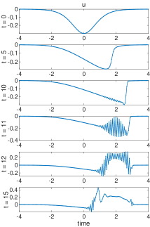
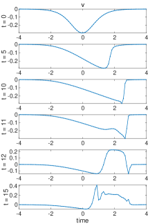
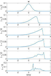
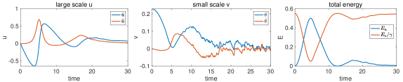
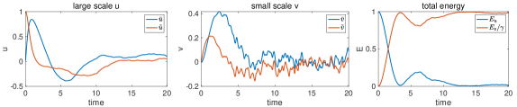
In the numerical illustrations of the two-layer L96 solutions of (4.2), we consider two initial values: i) zero large-scale state $u_{1}\left(0\right)=u_{2}\left(0\right)=0$ and continuous small-scale profile $v_{0}=0.3\mathrm{sech}^{2}\left(\frac{x}{2}\right)$ ; and ii) jump discontinuity at the two large-scale states $u_{1}\left(0\right)=1$ , $u_{2}\left(0\right)=-1$ and zero small scale $v_{0}\equiv 0$ . The same as the one-layer model case, we use the discretization points $L=256$ and the 4th-order Runge-Kutta method is used for the time integration. First, the time evolution of the large-scale states are shown in Figure 8. The large scale and small scale mean interacts nonlinearly in the starting time. It is observed in both test cases, the energy exchanges between the large and small scale states and finally mostly transfers to the small-scale state $v$ when strong chaotic behaviors are developed.

The small-scale solutions in the two test cases are compared in Figure 9 and Figure 10. From both initial values, oscillatory solutions in $v$ will be developed near the point $x=0$ due to the different forcing $u_{1}$ and $u_{2}$ exerted on $v$ from the left and right sides of the domain according to (4.2). It is observed the oscillations are moving to the left side of the discontinuity due to the wave group velocity $-c=-\frac{3}{2}\gamma\bar{v}$ consistent with the analysis in (4.13). We also approximate the period two solutions by $\eta=\frac{1}{3}\left(v_{l-1}+v_{l}+v_{l+1}\right)$ and $\xi=\frac{1}{3}\left(-\frac{1}{2}v_{l-1}+v_{l}-\frac{1}{2}v_{l+1}\right)$ . Notice that (4.9) gives the leading-order small-scale approximation since higher-order feedbacks from the large-scale states also have contributions to the two-layer model (4.2) besides the leading-order terms in the large-scale equation (4.8). The combination of multiple approximation and numerical effects makes it tricky to observe a clean period-three solution in the full two-layer model simulations. Still, in the region where oscillatory solutions start to develop, the three point averages $\eta,\xi$ demonstrate smoother solution except some small fluctuations due to the higher-order perturbations. This indicates the period-three behavior of the oscillatory solution along its way to fully chaotic dynamics.

5 Summary

We studied the development of chaotic behaviors commonly observed in the simulations of the Lorenz 96 systems through the approach of analyzing the convergence of discrete dispersive schemes. The final chaotic solution can be explained as a competition between the stable solution and unstable oscillatory solutions developed during the time evolution of the leading-order equations. Oscillations are shown to arise in the discrete L96 models when discontinuity is developed from the classical solution. We show that period-two oscillatory solutions exist in the modulation equation, while period-three oscillations may also occur in a weakly nonlinear analysis. Applying Strang’s convergence theorem to the regions of oscillatory solutions, we show that the particular modulation equations and asymptotic weakly nonlinear approximations characterize the period-two and period-three oscillations correspondingly. The analytical results are supported by direct numerical simulations in various parameter regimes of the one-layer and two-layer L96 models. The ideas can be also generalized to study the more complicated interactions of period-two and three oscillations that finally lead to the fully turbulent dynamics.

Acknowledgements

The research of D.Q. is partially supported by ONR grant N00014-24-1-2192 and NSF grant DMS-2407361. The research of J.-G. L. is partially supported under the NSF grant DMS-2106988.

References

[1] Rafail V Abramov and Andrew J Majda. Quantifying uncertainty for non-Gaussian ensembles in complex systems. SIAM Journal on Scientific Computing, 26(2):411–447, 2004.
[2] HM Arnold, IM Moroz, and TN Palmer. Stochastic parametrizations and model uncertainty in the Lorenz ’96 system. Philosophical Transactions of the Royal Society A: Mathematical, Physical and Engineering Sciences, 371(1991):20110479, 2013.
[3] Jacob Bedrossian, Alex Blumenthal, and Sam Punshon-Smith. A regularity method for lower bounds on the Lyapunov exponent for stochastic differential equations. Inventiones mathematicae, 227(2):429–516, 2022.
[4] Ibrahim Fatkullin and Eric Vanden-Eijnden. A computational strategy for multiscale systems with applications to Lorenz 96 model. Journal of Computational Physics, 200(2):605–638, 2004.
[5] Jonathan Goodman and Peter D Lax. On dispersive difference schemes. I. In Selected Papers Volume I, pages 545–567. Springer, 1988.
[6] Thomas Y Hou and Peter D Lax. Dispersive approximations in fluid dynamics. In Selected Papers Volume I, pages 568–607. Springer, 1991.
[7] Alireza Karimi and Mark R Paul. Extensive chaos in the Lorenz-96 model. Chaos: An interdisciplinary journal of nonlinear science, 20(4), 2010.
[8] Peter D Lax. On dispersive difference schemes. Physica D: Nonlinear Phenomena, 18(1-3):250–254, 1986.
[9] Peter D Lax and C David Levermore. The small dispersion limit of the Korteweg-de Vries equation. i. In Selected Papers Volume I, pages 463–500. Springer, 1983.
[10] C David Levermore and Jian-Guo Liu. Large oscillations arising in a dispersive numerical scheme. Physica D: Nonlinear Phenomena, 99(2-3):191–216, 1996.
[11] Jian-Guo Liu and Zhou Ping Xin. L¹-stability of stationary discrete shocks. Mathematics of computation, 60(201):233–244, 1993.
[12] Jian Guo Liu and Zhouping Xin. Nonlinear stability of discrete shocks for systems of conservation laws. Archive for rational mechanics and analysis, 125:217–256, 1993.
[13] Edward N Lorenz and Kerry A Emanuel. Optimal sites for supplementary weather observations: Simulation with a small model. Journal of the Atmospheric Sciences, 55(3):399–414, 1998.
[14] EN Lorenz. Predictability: A problem partly solved. Proceedings of the Seminar on Predictability, 1996.
[15] Andrew J Majda. Introduction to turbulent dynamical systems in complex systems. Springer, 2016.
[16] Andrew J Majda and Di Qi. Strategies for reduced-order models for predicting the statistical responses and uncertainty quantification in complex turbulent dynamical systems. SIAM Review, 60(3):491–549, 2018.
[17] Andrew J Majda and Di Qi. Linear and nonlinear statistical response theories with prototype applications to sensitivity analysis and statistical control of complex turbulent dynamical systems. Chaos: An Interdisciplinary Journal of Nonlinear Science, 29(10), 2019.
[18] Andrew J Majda and Ilya Timofeyev. Remarkable statistical behavior for truncated Burgers–Hopf dynamics. Proceedings of the National Academy of Sciences, 97(23):12413–12417, 2000.
[19] Dirk Olbers. A gallery of simple models from climate physics. In Stochastic Climate Models, pages 3–63. Springer, 2001.
[20] David Orrell. Model error and predictability over different timescales in the Lorenz ’96 systems. Journal of the atmospheric sciences, 60(17):2219–2228, 2003.
[21] Di Qi and Jian-Guo Liu. High-order moment closure models with random batch method for efficient computation of multiscale turbulent systems. Chaos: An Interdisciplinary Journal of Nonlinear Science, 33(10), 2023.
[22] Di Qi and Jian-Guo Liu. A random batch method for efficient ensemble forecasts of multiscale turbulent systems. Chaos: An Interdisciplinary Journal of Nonlinear Science, 33(2), 2023.
[23] Gilbert Strang. Accurate partial difference methods: II. non-linear problems. Numerische Mathematik, 6(1):37–46, 1964.
[24] Andrew Stuart and Anthony R Humphries. Dynamical systems and numerical analysis, volume 2. Cambridge University Press, 1998.
[25] Daniel S Wilks. Effects of stochastic parametrizations in the Lorenz ’96 system. Quarterly Journal of the Royal Meteorological Society: A journal of the atmospheric sciences, applied meteorology and physical oceanography, 131(606):389–407, 2005.
[26] Zhouping Xin. On the linearized stability of viscous shock profiles for systems of conservation laws. Journal of differential equations, 100(1):119–136, 1992.

	$\displaystyle\left\|\tilde{M}\left(t\right)\right\|$	$\displaystyle\leq\frac{2}{ah}\int_{0}^{t}e^{-\frac{2}{ah}\int_{s}^{t}\left(v_{h}\left(\tau\right)+\tilde{v}\left(\tau\right)h\right)d\tau}M_{h}\left(s\right)\left\|\tilde{v}\left(s\right)\right\|ds$
		$\displaystyle\leq\frac{2}{ah}\int_{0}^{t}e^{\frac{\lambda}{ah}s+C}M_{h}\left(s\right)\left\|\tilde{v}\left(s\right)\right\|ds$
		$\displaystyle\leq\frac{C}{h}\int_{0}^{t}\exp\left(-\frac{\lambda}{ah}s\right)ds\leq C^{\prime}.$