Outer Channel of DNA-Based Data Storage: Capacity and Efficient Coding Schemes

Xuan He, Yi Ding, Kui Cai, Guanghui Song, Bin Dai, and Xiaohu Tang This work was presented in part at [1]. DOI: 10.1109/ICCCWorkshops57813.2023.10233840

Abstract

In this paper, we consider the outer channel for DNA-based data storage, where each DNA string is either correctly transmitted, or being erased, or being corrupted by uniformly distributed random substitution errors, and all strings are randomly shuffled with each other. We first derive the capacity of the outer channel, which surprisingly implies that the uniformly distributed random substitution errors are only as harmful as the erasure errors. Next, we propose efficient coding schemes which encode the bits at the same position of different strings into a codeword. We compute the soft/hard information of each bit, which allows us to independently decode the bits within a codeword, leading to an independent decoding scheme. To improve the decoding performance, we measure the reliability of each string based on the independent decoding result, and perform a further step of decoding over the most reliable strings, leading to a joint decoding scheme. Simulations with low-density parity-check codes confirm that the joint decoding scheme can reduce the frame error rate by more than 3 orders of magnitude compared to the independent decoding scheme, and it can outperform the state-of-the-art decoding scheme in the literature in a wide parameter regions.

Index Terms:

Capacity, DNA-based data storage, joint decoding scheme, low-density parity-check (LDPC) code, outer channel.

I Introduction

Due to the increasing demand for data storage, DNA-based data storage systems have attracted significant attention, since they can achieve extremely high data storage capacity, with very long life duration and low maintenance cost [2, 3, 4]. A typical model for these systems is shown by Fig. 1 [5]. Due to biochemical constraints, the source data is stored in many short DNA strings in an unordered manner. A DNA string/strand/oligo can be missing or corrupted by insertion, deletion, and/or substitution errors during the synthesis, storage, and/or sequencing processes. Therefore, in typical DNA-based data storage systems, an inner code is used to detect/correct the errors within a string, whereas an outer code is used to recover the missing strings and correct the undetectable substitution errors from inner decoding.

In this paper, we focus on the outer code in Fig. 1. Thus, we adopt a simplified system model shown in Fig. 2, where the channel of interest, referred to as the outer channel, is the concatenation of channel-1 and channel-2. The input of channel-1 is an $n\times l$ binary matrix $\mathbf{X}$ , each row of which corresponds to a DNA string. Each row (NOT each bit) of $\mathbf{X}$ is correctly transmitted over channel-1 with probability $p_{c}$ , or erased with probability $p_{e}$ , or corrupted by length- $l$ uniformly distributed random substitution errors with probability $p_{s}$ , where $p_{c}+p_{e}+p_{s}=1$ . After that, the rows at the output of channel-1 are randomly shuffled with each other by channel-2. In this case, we indeed view the inner code as a part of channel-1 such that only the valid (but possibly incorrect) inner codewords from the inner decoding form the output of channel-1. It explains why channel-1 adds erasure and substitution errors to a whole row of $\mathbf{X}$ instead of its bits independently.

We say that the rate $R$ (number of information bits stored in per transmitting coded bit) is achievable if there exists a code with rate $R$ such that the decoding error probability tends to $0$ as $n\to\infty$ , and the channel capacity refers to the maximum achievable code rate. In this paper, we are interested in both computing the capacity and developing practical and efficient coding schemes for the outer channel.

Refer to caption — Figure 1: A typical system model for DNA-based data storage [5].

I-A Related Work

TABLE I: Comparison between the existing work and this work

Work	Channel model	Difference
this work	outer channel
[1]	outer channel	no capacity result
[5]	concatenation channel	no erasure errors; no capacity result
[6]	noisy permutation channel	no erasure errors; modified capacity for $n\to\infty$ and fixed $l$ (i.e., $\beta\to 0$ )
[7]	noise-free shuffling-sampling channel	no sustitution errors
[7, 8, 9]	noisy shuffling-sampling channels	bits within a string independently suffer from substitution errors

This is an extended work of its conference version [1]. In [1], we proposed an efficient coding scheme for the outer channel. In this work, we further prove the capacity of the outer channel.

The outer channel is almost the same as the concatenation channel in [5, Fig. 2(a)], except that we additionally consider erasure errors in this paper. In [5], fountain codes [10, 11] were used as the outer codes, and an efficient decoding scheme, called basis-finding algorithm (BFA), was proposed for fountain codes. BFA can also work for the outer channel in this paper when fountain codes are being used, and it serves as a benchmark for the simulation results later in Section V. However, the capacity of the concatenation channel has not been discussed in [5].

In [6, Fig. 2], Makur considered a noisy permutation channel which essentially is the same as the concatenation channel in [5, Fig. 2(a)]. Define

\beta\triangleq\lim_{n\to\infty}\frac{l}{\log_{2}n},

(1)

in which $n$ and $l$ are the number of rows and number of columns in $\mathbf{X}$ , respectively. Makur modified the conventional definition of channel capacity and computed the modified capacity for $n\to\infty$ and fixed $l$ (i.e., $\beta\to 0$ in this case). However, we will soon see that the (conventional) capacity of the outer channel equals zero for $\beta\leq 1$ , and we thus aim to compute the capacity of the the outer channel for $\beta>1$ in this paper.

In [7], Shomorony and Heckel considered a noise-free shuffling-sampling channel, which can also be described as the concatenation of two sub-channels. The second sub-channel is the same as our channel-2. The first sub-channel outputs some noise-free copies of rows of the input $\mathbf{X}$ , where the number of copies follows a certain probability distribution, e.g, the Bernoulli distribution. Let $p_{erasure}$ denote the probability that the first sub-channel does not output any copy for a row of $\mathbf{X}$ . According to [7, Theorem 1], the noise-free shuffling-sampling channel has capacity

C_{nf}=(1-p_{erasure})(1-1/\beta),

(2)

as long as $\beta>1$ , and $C_{nf}=0$ for $\beta\leq 1$ . In (2), $1-1/\beta$ can be understood as the loss due to the random permutation of the second sub-channel, which implies that index-based coding scheme that uses $\log_{2}n$ bits for uniquely labelling each row of $\mathbf{X}$ is optimal [7].

Shomorony and Heckel [7] additionally studied a noisy shuffling-sampling channel. In [8] and [9], more noisy shuffling-sampling channels (also called noisy drawing channels) were considered. However, these channels include discrete memoryless channels (e.g., binary symmetric channel (BSC)), which independently add substitution errors to each bit within a row of $\mathbf{X}$ . This is the key difference from our channel-1 which does not independently add substitution errors to each bit within a row.

We summarize the differences between the existing work and this work in Table I. As can be seen from Table I, the capacity of the outer channel is not clear for $\beta>1$ up till now.

I-B Main Contributions

This paper provides two main contributions. Our first contribution is to derive the capacity $C$ of the outer channel, given by the following theorem.

Theorem 1.

The capacity of the outer channel is

C=p_{c}(1-1/\beta),

(3)

as long as $\beta>1$ , and $C=0$ for $\beta\leq 1$ .

From [7], it is known that $C=0$ for $\beta\leq 1$ . Therefore, we focus on $\beta>1$ by default from now on except where otherwise stated. Intuitively, the received rows in $\mathbf{Z}$ that are corrupted by uniformly distributed random substitution errors can provide no (at most negligible) information about $\mathbf{X}$ . Suppose there is a genie-aided outer channel which has a genie to identify and remove these incorrect rows, then the channel becomes a type of noise-free shuffling-sampling channel in [7] with $p_{erasure}=p_{e}+p_{s}$ . According to (2), its capacity is given by $C_{nf}=(1-p_{erasure})(1-1/\beta)=p_{c}(1-1/\beta)$ . In contrast to (3), it implies that the uniformly distributed random substitution errors are as harmful as erasure errors when $\beta>1$ and $n\to\infty$ (recall that we compute capacity for $n\to\infty$ ). This motivates us to develop efficient decoding schemes by treating incorrect rows as erased ones in Section IV, i.e., identify and remove the incorrect rows.

Our second contribution is to develop an efficient coding scheme for the outer channel. More specifically, our encoding scheme is first to choose a block error-correction code (ECC) to encode each column of $\mathbf{X}$ as a codeword so as to tackle erasure and substitution errors from channel-1, and then to add a unique address to each row of $\mathbf{X}$ so as to combat disordering of channel-2. Our decoding scheme is first to derive the soft/hard information for each data bit in $\mathbf{X}$ . It allows us to decode each column of $\mathbf{X}$ independently, leading to an independent decoding scheme. However, this scheme may not be very efficient since it requires the successful decoding of all columns to fully recover $\mathbf{X}$ . Therefore, we further measure the reliability of the received rows of $\mathbf{X}$ based on the independent decoding result. Then, we take the most reliable received rows to recover $\mathbf{X}$ like under the erasure channel, leading to an efficient joint decoding scheme. Simulations with low-density parity-check (LDPC) codes [12] show that the joint decoding scheme can reduce the frame error rate (FER) by more than 3 orders of magnitude compared to the independent decoding scheme. Moreover, it demonstrates that the joint decoding scheme and the BFA can outperform each other under different parameter region.

I-C Organization

The remainder of this paper is organized as follows. Section II illustrates the outer channel and the encoding scheme. Section III proves Theorem 1. Section IV develops both the independent and joint decoding schemes. Section V presents the simulation results. Finally, Section VI concludes this paper.

I-D Notations

In this paper, we generally use non-bold lowercase letters for scalars (e.g., $n$ ), bold lowercase letters for (row) vectors (e.g., $\mathbf{x}$ ), bold uppercase letters for matrices (e.g., $\mathbf{X}$ ), non-bold uppercase letters for random variables and events (e.g., $E$ ), and calligraphic letters for sets (e.g., $\mathcal{Z}$ ). For any $n\times l$ matrix $\mathbf{X}$ , we refer to its $i$ -th row and $(i,j)$ -th entry by $\mathbf{x}_{i}$ and $x_{i,j}$ , respectively, i.e., $\mathbf{X}=[(\mathbf{x}_{i}^{\mathrm{T}})_{1\leq i\leq n}]^{\mathrm{T}}=({x}_{i,j})_{1\leq i\leq n,1\leq j\leq l}$ , where $(\cdot)^{\mathrm{T}}$ is the transpose of a vector or matrix. For any two matrices $\mathbf{X}$ and $\mathbf{Y}$ , denote $\mathbf{X}\cap\mathbf{Y}$ as the set intersection of their rows (only one copy of the same rows is kept). For any two events $E_{1}$ and $E_{2}$ , denote $E_{1}\vee E_{2}$ as their union, and denote $\mathbb{P}(E_{1})$ as the probability that $E_{1}$ happens. Denote $\mathbb{F}_{2}\triangleq\{0,1\}$ as the binary field and $[n]\triangleq\{1,2,\ldots,n\}$ for any positive integer $n$ .

II System Model and Encoding Scheme

Recall that we focus on the outer code in Fig. 1. Therefore, motivated by [5], we consider the simplified system model in Fig. 2, where the encoder and decoder are related to the outer code, the inner code is viewed as a part of channel-1, and channel-2 is to randomly shuffle DNA strings with each other. The outer channel considered in this paper is the concatenation of channel-1 and channel-2.

More specifically, first, the data matrix $\mathbf{U}\in\mathbb{F}_{2}^{k\times w}$ is encoded as $\mathbf{X}\in\mathbb{F}_{2}^{n\times l}$ , where each row of $\mathbf{X}$ corresponds to a DNA string in DNA-based data storage systems. Then, the rows of $\mathbf{X}$ are transmitted over channel-1 and received one-by-one in order. For each $i\in[n]$ , the $i$ -th received row $\mathbf{y}_{i}\in\mathbf{Y}$ indeed corresponds to the inner decoding result of the $i$ -th transmitted row $\mathbf{x}_{i}\in\mathbf{X}$ . Thus, we regard $\mathbf{x}_{i}$ (instead of each its bit) as a whole to be transmitted over channel-1. Particularly, $\mathbf{y}_{i}$ can be classified into three cases:

•

$\mathbf{y}_{i}=\mathbf{x}_{i}$ : The inner decoding of $\mathbf{x}_{i}$ succeeds.
•

$\mathbf{y}_{i}=?$ : The inner decoding of $\mathbf{x}_{i}$ fails to give a valid inner codeword such that $\mathbf{y}_{i}$ is regarded as an erasure error. This case can be caused by either that $\mathbf{x}_{i}$ is corrupted by too many errors or that $\mathbf{x}_{i}$ is missing during the synthesizing, storage, or sequencing process.
•

$\mathbf{y}_{i}\in\mathbb{F}_{2}^{l}\setminus\{\mathbf{x}_{i}\}$ : The inner decoding of $\mathbf{x}_{i}$ gives a valid but incorrect inner codeword, i.e., an undetectable error happens.

Accordingly, we model the transition probability of channel-1 by

\mathbb{P}(\mathbf{y}_{i}|\mathbf{x}_{i})=\begin{cases}p_{c},&\mathbf{y}_{i}=\mathbf{x}_{i},\\ p_{e},&\mathbf{y}_{i}=?,\\ p_{s}/(2^{l}-1),&\mathbf{y}_{i}=\mathbf{e}\in\mathbb{F}_{2}^{l}\setminus\{\mathbf{x}_{i}\},\end{cases}

(4)

where $p_{c}+p_{e}+p_{s}=1$ . Note that in practice, $p_{c}$ should be large enough to ensure the success of the outer decoding. Thus, we further require

p_{c}>p_{s}/(2^{l}-1).

(5)

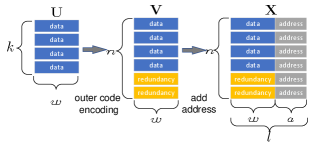
Next, $\mathbf{Y}$ is transmitted over channel-2 where its rows are shuffled uniformly at random to form $\mathbf{Z}$ . For convenience, we regard both $\mathbf{Y}$ and $\mathbf{Z}$ having $n$ rows in which any erased rows are represented by ‘?’. Finally, the decoder gives an estimation $\widehat{\mathbf{U}}$ of $\mathbf{U}$ based on $\mathbf{Z}$ .

To protect against the above channel errors, we adopt the encoder illustrated by Fig. 3 to convert the data matrix $\mathbf{U}\in\mathbb{F}_{2}^{k\times w}$ into the encoded matrix $\mathbf{X}\in\mathbb{F}_{2}^{n\times l}$ with the following two steps:

•

A (binary) ECC of block length- $n$ is chosen to encode each column of $\mathbf{U}$ as a column (codeword) of $\mathbf{V}\in\mathbb{F}_{2}^{n\times w}$ , so as to tackle the erasure errors and substitution errors from channel-1. Random ECCs will be used for proving the capacity and any excellent linear ECCs (e.g., LDPC codes) can be used in practical scenarios.
•

A unique address of bit-width $a\triangleq l-w\geq\lceil\log_{2}n\rceil$ is added to the tail of each row of $\mathbf{V}$ , leading to $\mathbf{X}$ , so as to combat the disordering of channel-2. Without loss of generality (WLOG), we set the address of $\mathbf{x}_{i}$ as $i$ for any $i\in[n]$ . Note that given $n$ , increasing $a$ can reduce the probability that an address is changed to a valid address when substitution errors occur. Since for DNA-based data storage, we can simply discard the received rows without valid addresses, increasing $a$ is equivalent to reducing $p_{s}$ and increasing $p_{e}$ in our system model. Thus, we use the minimum $a$ by default, i.e., $a=\lceil\log_{2}n\rceil$ . By convenience, we refer to the first $w$ columns and the last $a$ columns of $\mathbf{X}$ by data and address, respectively.

Example 1.

This example shows the encoding process of Fig. 3. Consider the following source data matrix:

\mathbf{U}=\left[\begin{array}[]{c c c c}0&0&1&1\\ 0&1&0&1\\ \end{array}\right].

(6)

We systematically encode each column of $\mathbf{U}$ by an $(n=6,k=2)$ linear block ECC with a minimum distance of $4$ and with the following parity-check matrix:

\mathbf{H}=\left[\begin{array}[]{c c c c c c c}1&0&1&0&0&0\\ 1&1&0&1&0&0\\ 1&1&0&0&1&0\\ 0&1&0&0&0&1\\ \end{array}\right].

(7)

We then get

\mathbf{V}=\left[\begin{array}[]{c}\mathbf{U}\\ \hline\cr\mathbf{P}\\ \end{array}\right]=\left[\begin{array}[]{c c c c}0&0&1&1\\ 0&1&0&1\\ \hline\cr 0&0&1&1\\ 0&1&1&0\\ 0&1&1&0\\ 0&1&0&1\\ \end{array}\right],

(8)

where $\mathbf{P}$ denotes the parity-check part. For each $i\in[n]$ , adding address $i$ (of $a=3$ bits) into the $i$ -th row of $\mathbf{V}$ leads to

\mathbf{X}=[\mathbf{V|\mathbf{A}}]=\left[\begin{array}[]{c c c c | c c c}0&0&1&1&0&0&1\\ 0&1&0&1&0&1&0\\ \hline\cr 0&0&1&1&0&1&1\\ 0&1&1&0&1&0&0\\ 0&1&1&0&1&0&1\\ 0&1&0&1&1&1&0\\ \end{array}\right],

(9)

where $\mathbf{A}$ denotes the address part.

III Proof of Theorem 1

The code rate of the system in Fig. 2 is

R\triangleq\frac{kw}{nl}.

Recall that $\beta=\lim_{n\to\infty}l/\log_{2}n$ . According to [7], the outer channel has capacity $C=0$ for $\beta\leq 1$ . Therefore, to prove Theorem 1, we only need to further show the following two lemmas.

Lemma 1 (achivability).

For $\beta>1$ and arbitrarily small fixed $\epsilon>0$ , the following code rate is achievable:

R=(p_{c}-2\epsilon)(1-1/\beta).

(10)

Lemma 2 (converse).

For $\beta>1$ and arbitrarily small fixed $\delta>0$ , as $n\to\infty$ , any achievable code rate $R$ satisfies

R\leq(p_{c}+\delta)(1-1/\beta).

(11)

III-A Proof of Lemma 1

To prove Lemma 1, we only need to show that for $\beta>1$ and arbitrarily small fixed $\epsilon>0$ , there is a code with rate $R=(p_{c}-2\epsilon)(1-1/\beta)$ such that the decoding error probability $\mathbb{P}(\widehat{\mathbf{U}}\neq\mathbf{U})\to 0$ as $n\to\infty$ . WLOG, assume $n(p-2\epsilon)$ , $n(p-\epsilon)$ , and $\log_{2}n$ are integers. Let $k=n(p-2\epsilon)$ and $a=\log_{2}n$ such that the code rate is $R=kw/(nl)=k(l-a)/(nl)=(p_{c}-2\epsilon)(1-1/\beta)$ . Define $N\triangleq 2^{kw}$ for convenience.

Encoding scheme: We choose $N$ matrices $\mathbf{V}_{1},\mathbf{V}_{2},\ldots,\mathbf{V}_{N}$ from $\mathbb{F}_{2}^{n\times w}$ uniformly at random to form the codebook of ECC, and adopt the encoding scheme in Fig. 3. More specifically, for any $i\in[N]$ , we first encode the $i$ -th data matrix $\mathbf{U}_{i}\in\mathbb{F}_{2}^{k\times w}$ to $\mathbf{V}_{i}\in\mathbb{F}_{2}^{n\times w}$ , and then add address $j$ to the $j$ -th row of $\mathbf{V}_{i}$ for all $j\in[n]$ to form the encoded matrix $\mathbf{X}_{i}\in\mathbb{F}_{2}^{k\times l}$ .

Decoding scheme: After receiving $\mathbf{Z}$ , if there exists a unique $i\in[N]$ such that $|\mathbf{X}_{i}\cap\mathbf{Z}|\geq n(p_{c}-\epsilon)$ , where $\mathbf{X}_{i}\cap\mathbf{Z}$ is the set intersection of $\mathbf{X}_{i}$ ’s rows and $\mathbf{Z}$ ’s rows, then return $\widehat{\mathbf{U}}=\mathbf{U}_{i}$ as the decoding result; otherwise, return $\widehat{\mathbf{U}}=?$ to indicate a decoding failure.

Decoding error probability: For any $i\in[N]$ , define $E_{i}$ as the event of $|\mathbf{X}_{i}\cap\mathbf{Z}|\geq n(p_{c}-\epsilon)$ and $\bar{E}_{i}$ as the event of $|\mathbf{X}_{i}\cap\mathbf{Z}|<n(p_{c}-\epsilon)$ . WLOG, assume the source data matrix $\mathbf{U}=\mathbf{U}_{1}$ and the transmitted encoded matrix $\mathbf{X}=\mathbf{X}_{1}$ . Then, the decoding error probability is given by

	$\displaystyle\mathbb{P}(\widehat{\mathbf{U}}\neq\mathbf{U}_{1})$	$\displaystyle=\mathbb{P}(\bar{E}_{1}\vee E_{2}\vee E_{3}\vee\cdots\vee E_{N})$
		$\displaystyle\leq\mathbb{P}(\bar{E}_{1})+\sum_{i=2}^{N}\mathbb{P}(E_{i})$		(12)

We first bound $\mathbb{P}(\bar{E}_{1})$ . Let $n_{c}$ denote the number of correctly transmitted rows of $\mathbf{X}_{1}$ . We have $|\mathbf{X}_{1}\cap\mathbf{Z}|\geq n_{c}$ . Then,

$\displaystyle\mathbb{P}(\bar{E}_{1})$	$\displaystyle=\mathbb{P}(\|\mathbf{X}_{1}\cap\mathbf{Z}\|<n(p_{c}-\epsilon))$
	$\displaystyle\leq\mathbb{P}(n_{c}\leq n(p_{c}-\epsilon))$
	$\displaystyle\leq e^{-2n\epsilon^{2}},$	(13)

where the last inequality is based on Hoeffding’s inequality [13].

We now bound $\mathbb{P}(E_{i})$ for any $2\leq i\leq N$ . Recall that any erased one of $n$ rows in $\mathbf{Z}$ is represented by ‘?’. Thus, there are $S\triangleq\binom{n}{n(p_{c}-\epsilon)}$ many ways to select $n(p_{c}-\epsilon)$ rows from $\mathbf{Z}$ to form submatrices which are denoted by $\mathbf{S}_{j},j\in[S]$ . Define $E_{i,j}$ as the event of $|\mathbf{X}_{i}\cap\mathbf{S}_{j}|=n(p_{c}-\epsilon)$ . $E_{i,j}$ happens if and only if (iff) for all $h\in[n(p_{c}-\epsilon)]$ , $\mathbf{S}_{j}$ ’s $h$ -th row $\mathbf{s}_{h}$ has a unique address $a_{h}\in[n]$ and $\mathbf{s}_{h}$ equals $\mathbf{X}_{i}$ ’s $a_{h}$ -th row. Given that $\mathbf{s}_{h}$ has a unique address $a_{h}\in[n]$ , $\mathbf{s}_{h}$ equals $\mathbf{X}_{i}$ ’s $a_{h}$ -th row with probability $2^{-w}$ . Thus, $\mathbb{P}(E_{i,j})\leq 2^{-wn(p_{c}-\epsilon)}$ , leading to

$\displaystyle\mathbb{P}(E_{i})$	$\displaystyle=\mathbb{P}(\vee_{j=1}^{S}E_{i,j})$
	$\displaystyle\leq\sum_{j=1}^{S}\mathbb{P}(E_{i,j})$
	$\displaystyle\leq S\cdot 2^{-wn(p_{c}-\epsilon)}$
	$\displaystyle\leq 2^{n-wn(p_{c}-\epsilon)}.$	(14)

At this point, substituting (III-A) and (III-A) into (III-A) results in

$\displaystyle\mathbb{P}(\widehat{\mathbf{U}}\neq\mathbf{U}_{1})$	$\displaystyle\leq\mathbb{P}(\bar{E}_{1})+\sum_{i=2}^{N}\mathbb{P}(E_{i})$
	$\displaystyle\leq e^{-2n\epsilon^{2}}+(N-1)2^{n-wn(p_{c}-\epsilon)}$
	$\displaystyle\leq e^{-2n\epsilon^{2}}+2^{kw+n-wn(p_{c}-\epsilon)}$
	$\displaystyle=e^{-2n\epsilon^{2}}+2^{n(p_{c}-2\epsilon)w+n-wn(p_{c}-\epsilon)}$
	$\displaystyle=e^{-2n\epsilon^{2}}+2^{n-n\epsilon w}$
	$\displaystyle=e^{-2n\epsilon^{2}}+2^{n-n\epsilon(\beta-1)\log n}$
	$\displaystyle=0,$	(15)

where the last equality holds because $\epsilon$ is fixed, $\beta>1$ , and $n\to\infty$ . This completes the proof.

III-B Proof of Lemma 2

Note that

I(\mathbf{U};\widehat{\mathbf{U}})+H(\mathbf{U}|\widehat{\mathbf{U}})=H(\mathbf{U})=kw=nlR,

(16)

where $I$ is the mutual information function and $H$ is the entropy function. As $\mathbf{U}\rightarrow\mathbf{X}\rightarrow\mathbf{Z}\rightarrow\widehat{\mathbf{U}}$ forms a Markov chain, $I(\mathbf{U};\widehat{\mathbf{U}})\leq I(\mathbf{X};\mathbf{Z})$ by the data processing inequality [14]. Meanwhile, according to Fano’s inequality [14], we have $H(\mathbf{U}|\widehat{\mathbf{U}})\leq 1+\mathbb{P}(\mathbf{U}\neq\widehat{\mathbf{U}})\log_{2}(|\mathcal{U}|)$ , where $\mathcal{U}$ is the set that $\mathbf{U}$ takes values from and $|\mathcal{U}|=2^{nlR}$ in this paper. Therefore, (16) becomes

	$\displaystyle nlR$	$\displaystyle=I(\mathbf{U};\widehat{\mathbf{U}})+H(\mathbf{U}\|\widehat{\mathbf{U}})$
		$\displaystyle\leq I(\mathbf{X};\mathbf{Z})+1+\mathbb{P}(\mathbf{U}\neq\widehat{\mathbf{U}})nlR,$		(17)

Since we consider $\mathbb{P}(\mathbf{U}\neq\widehat{\mathbf{U}})\to 0$ as $n\to\infty$ in (III-B), to prove Lemma 2, it suffices to show

I(\mathbf{X};\mathbf{Z})\leq(p_{c}+\delta)(1-1/\beta)nl+o(nl).

(18)

To this end, we partition $\mathbf{Z}$ into two submatrices $\mathbf{S}$ and $\bar{\mathbf{S}}$ which consist of the rows in $\mathbf{Z}$ corrupted by uniformly distributed random substitution errors and the remaining rows, respectively. Note that the order of the rows in $\bar{\mathbf{S}}$ and $\mathbf{S}$ does not matter. We have

I(\mathbf{X};\mathbf{Z})=I(\mathbf{X};\bar{\mathbf{S}})+I(\mathbf{X};\mathbf{S}|\bar{\mathbf{S}}).

(19)

We first bound $I(\mathbf{X};\bar{\mathbf{S}})$ in (19). Since $\bar{\mathbf{S}}$ only contains correctly received rows and erased rows, $\bar{\mathbf{S}}$ can be regarded as the output of the noise-free shuffling-sampling channel [7], where each row of $\mathbf{X}$ is either sampled once with probability $p_{c}$ or never sampled with probability $1-p_{c}$ . Therefore, using a similar proof as [7, Section III-B] yields

I(\mathbf{X};\bar{\mathbf{S}})\leq H(\bar{\mathbf{S}})\leq(p_{c}+\delta)(1-1/\beta)nl+o(nl).

(20)

We now bound $I(\mathbf{X};\mathbf{S}|\bar{\mathbf{S}})$ in (19) based on

I(\mathbf{X};\mathbf{S}|\bar{\mathbf{S}})=H(\mathbf{S}|\bar{\mathbf{S}})-H(\mathbf{S}|\mathbf{X},\bar{\mathbf{S}}).

(21)

Denote $J$ as the number of rows in $\mathbf{S}$ . We have

$\displaystyle H(\mathbf{S}\|\bar{\mathbf{S}})$	$\displaystyle\overset{(i)}{=}H(\mathbf{S}\|\bar{\mathbf{S}},J)$
	$\displaystyle\leq H(\mathbf{S}\|J)$
	$\displaystyle\overset{(ii)}{\leq}\sum_{j=1}^{n}\mathbb{P}(J=j)jl$
	$\displaystyle=p_{s}nl,$	(22)

where $(i)$ follows the fact that $J$ is specified by $\bar{\mathbf{S}}$ , and $(ii)$ holds since given $J=j$ , $\mathbf{S}$ consists of ${jl}$ bits. Moreover, for any $i\in[J]$ , suppose the $i$ -th row $\mathbf{s}_{i}$ of $\mathbf{S}$ came from $\mathbf{x}_{f_{i}}$ . Let $\mathbf{f}\triangleq(f_{1},f_{2},\ldots,f_{J})$ . We have

$\displaystyle H(\mathbf{S}\|\mathbf{X},\bar{\mathbf{S}})$	$\displaystyle=H(\mathbf{S}\|\mathbf{X},\bar{\mathbf{S}},J)$
	$\displaystyle\geq H(\mathbf{S}\|\mathbf{X},\bar{\mathbf{S}},J,\mathbf{f})$
	$\displaystyle\overset{(iii)}{=}\sum_{j=1}^{n}\mathbb{P}(J=j)\sum_{i=1}^{j}H(\mathbf{s}_{i}\|\mathbf{x}_{f_{i}})$
	$\displaystyle=p_{s}n\log_{2}(2^{l}-1),$	(23)

where $(iii)$ holds because given $(\mathbf{X},J,\mathbf{f})$ , for any $i\in[J]$ , the $i$ -th row $\mathbf{s}_{i}$ of $\mathbf{S}$ only relates to $\mathbf{x}_{f_{i}}$ , and $\mathbf{s}_{i}$ has $2^{l}-1$ equiprobable choices according to (4). By applying (III-B) and (III-B) to (21), we have

I(\mathbf{X};\mathbf{S}|\bar{\mathbf{S}})\leq-\log_{2}(1-2^{-l})=o(1).

(24)

Finally, by substituting (20) and (24) into (19) yielding (18), the proof is completed.

IV Decoding Scheme

In this section, we first derive the soft information $\mathbf{M}=(m_{i,j})_{1\leq i\leq n,1\leq j\leq w}$ and hard information $\widehat{\mathbf{M}}=(\widehat{m}_{i,j})_{1\leq i\leq n,1\leq j\leq w}$ of each bit in $\mathbf{V}$ . This allows us to decode each column of $\mathbf{V}$ independently, leading to the independent decoding scheme. Next, in view that it requires the successful decoding of all columns to fully recover $\mathbf{V}$ (as well as $\mathbf{U}$ and $\mathbf{X}$ ), we propose an enhanced joint decoding scheme, which measures the reliability of rows of $\mathbf{Z}$ based on the independent decoding result and takes the most reliable rows for a further step of decoding.

Given any $i\in[n]$ and $j\in[w]$ , we begin with the computation of the soft information $m_{i,j}$ of $v_{i,j}\in\mathbf{V}$ . Conventionally, we should define $m_{i,j}\triangleq\mathbb{P}(v_{i,j}=0\mid\mathbf{Z})/\mathbb{P}(v_{i,j}=1\mid\mathbf{Z})$ . In fact, $m_{i,j}$ is only related to $\mathbf{y}_{i}$ . But the problem is that we do not know $\mathbf{y}_{i}$ corresponds to which row in $\mathbf{Z}$ due to the random permutation of channel-2, making it hard to compute $m_{i,j}$ exactly. Note from (4) that, if $\mathbf{y}_{i}$ is erased or corrupted by random substitution errors such that its address is not $i$ any more, no (or at most negligible) information about $v_{i,j}$ can be inferred from $\mathbf{y}_{i}$ even if we can figure out which row in $\mathbf{Z}$ corresponds to $\mathbf{y}_{i}$ . Therefore, it is reasonable to reduce the computation of $m_{i,j}$ from $\mathbf{Z}$ to the rows with address $i$ . Accordingly, we define

m_{i,j}\triangleq\frac{\mathbb{P}(v_{i,j}=0\mid t,t_{0})}{\mathbb{P}(v_{i,j}=1\mid t,t_{0})},

(25)

where $t$ denotes the number of rows in $\mathbf{Z}$ with address $i$ , among which there are $t_{0}$ rows with the $j$ -th bit being $0$ . Based on (25), $m_{i,j}$ can be computed by the following proposition.

Proposition 1.

$\displaystyle m_{i,j}=$	$\displaystyle\big{(}2t_{0}(1-q)(p_{1}+p_{4})+(n-t)q(p_{2}+p_{3})$
	$\displaystyle\quad+2(t-t_{0})(1-q)p_{5}\big{)}$
	$\displaystyle\big{/}\big{(}2(t-t_{0})(1-q)(p_{1}+p_{4})$
	$\displaystyle\quad+(n-t)q(p_{2}+p_{3})+2t_{0}(1-q)p_{5}\big{)},$	(26)

where

q\triangleq p_{s}2^{l-a}/(2^{l}-1)

(27)

and

p_{b}\triangleq\begin{cases}p_{c},&b=1,\\ p_{e},&b=2,\\ p_{s}(2^{l}-2^{l-a})/(2^{l}-1),&b=3,\\ p_{s}(2^{l-a-1}-1)/(2^{l}-1),&b=4,\\ p_{s}2^{l-a-1}/(2^{l}-1),&b=5.\end{cases}

(28)

Proof:

See Appendix A. ∎

Based on Proposition 1, it is natural to define the hard information of $v_{i,j}$ by:

\widehat{m}_{i,j}\triangleq\begin{cases}?,&m_{i,j}=1,\\ 0,&m_{i,j}>1,\\ 1,&m_{i,j}<1.\end{cases}

(29)

The following corollary simplifies (29).

Corollary 1.

\widehat{m}_{i,j}=\begin{cases}?,&t_{0}=t/2,\\ 0,&t_{0}>t/2,\\ 1,&t_{0}<t/2.\end{cases}

(30)

Proof.

By Proposition 1, we have

$\displaystyle m_{i,j}\geq 1$	$\displaystyle\iff(2t_{0}-t)(p_{1}+p_{4}-p_{5})\geq 0$
	$\displaystyle\iff(2t_{0}-t)(p_{c}-p_{s}/(2^{l}-1))\geq 0$
	$\displaystyle\iff 2t_{0}-t\geq 0,$	(31)

where the last step is due to (5) and the equality holds iff $t_{0}=t/2$ . ∎

Eqn. (30) is quite intuitive since it coincides with the majority decoding result. Hence, it somehow verifies the correctness of (1). Given the soft information in (1) or hard information in (30), it is able to perform decoding independently for each column of $\mathbf{V}$ . However, this decoding scheme can fully recover $\mathbf{V}$ only if the decoding for each column succeeds. This condition is generally too strong to achieve a desired decoding performance, as illustrated by the following example.

Example 2.

Continued with Example 1. Suppose the $\mathbf{X}$ in (9) is transmitted over channel-1 and the output is

\mathbf{Y}=\left[\begin{array}[]{c c c c | c c c}0&0&\underline{0}&\underline{0}&0&\underline{1}&\underline{0}\\ 0&1&0&1&0&1&0\\ \hline\cr\underline{1}&\underline{1}&1&1&0&1&1\\ 0&1&1&0&1&0&0\\ 0&1&1&0&1&0&1\\ 0&1&0&1&1&1&0\\ \end{array}\right],

(32)

where the underlined bits are flipped by channel-1. That is, $\mathbf{y}_{1}$ is corrupted by substitution errors and its address changes to $\mathbf{y}_{2}$ ’s address; $\mathbf{y}_{3}$ is also corrupted by substitution errors but its address does not change. Assume $\mathbf{Z}=\mathbf{Y}$ for convenience (but the decoder does not know the correspondence between the rows of $\mathbf{Z}$ and $\mathbf{Y}$ ).

We compute the hard information of $\mathbf{V}$ by (30), leading to

\widehat{\mathbf{M}}=\left[\begin{array}[]{c c c c}?&?&?&?\\ 0&?&0&?\\ \hline\cr{\color[rgb]{1,0,0}\mathbf{1}}&{\color[rgb]{1,0,0}\mathbf{1}}&1&1\\ 0&1&1&0\\ 0&1&1&0\\ 0&1&0&1\\ \end{array}\right],

(33)

where the bold red bits are different from the corresponding bits of $\mathbf{V}$ in (8). For examples, $\widehat{m}_{1,1}=?$ since $\mathbf{Z}$ does not have a row with address 1; $\widehat{m}_{2,2}=?$ since $\mathbf{Z}$ has $t=2$ rows with address 2 and their second bits differ from each other, i.e., $t_{0}=1$ . It is natural to decode each column of $\widehat{\mathbf{M}}$ as the nearest codeword (in terms of Hamming distance), leading to

\tilde{\mathbf{V}}=\left[\begin{array}[]{c c c c}0&?&1&1\\ 0&?&0&1\\ \hline\cr 0&?&1&1\\ 0&?&1&0\\ 0&?&1&0\\ 0&?&0&1\\ \end{array}\right],

(34)

where the second column corresponds to a decoding failure since both $(0,1,0,1,1,1)^{\mathrm{T}}$ and $(1,0,1,1,1,0)^{\mathrm{T}}$ are the nearest codewords of the second column of $\widehat{\mathbf{M}}$ . Thus, the independent decoding scheme fails to fully recover $\mathbf{V}$ .

We find that in Example 2, all the known bits in $\tilde{\mathbf{V}}$ are correct. In a general situation, the known bits in $\tilde{\mathbf{V}}$ should also be correct with a high probability. We thus assume

\mathbb{P}(\tilde{v}_{i,j}=v_{i,j})>1/2,\quad\forall\tilde{v}_{i,j}\in\tilde{\mathbf{V}}\text{~{}and~{}}\tilde{v}_{i,j}\in\mathbb{F}_{2}.

(35)

Consequently, for a non-erased correct (resp. incorrect) row in $\mathbf{Z}$ with address $i\in[n]$ , it generally has a relatively small (resp. large) distance from $\tilde{\mathbf{v}}_{i}$ . This provides a way to measure the reliability of rows of $\mathbf{Z}$ . We can then perform a further step of decoding over the most reliable rows of $\mathbf{Z}$ like under the erasure channel, as shown by Algorithm 1. In the following, we give more explanations (including Example 3) for Algorithm 1.

Algorithm 1 Joint decoding scheme

\mathbf{Z}=[(\mathbf{z}_{i}^{\mathrm{T}})_{1\leq i\leq n}]^{\mathrm{T}}=({z}_{i,j})_{1\leq i\leq n,1\leq j\leq l}

\widehat{\mathbf{U}}

1: Calculate the soft/hard information of

v_{i,j},i\in[n],j\in[w]

based on (1)/(30).

2: Decode each column of

\mathbf{V}

independently and denote the result by

\tilde{\mathbf{V}}=(\tilde{v}_{i,j})_{1\leq i\leq n,1\leq j\leq w}

, where

\tilde{v}_{i,j}\in\mathbb{F}_{2}

if decoding the

j

-th column of

\mathbf{V}

gives a valid codeword and

\tilde{v}_{i,j}=?

otherwise.

3: For each

i\in[n]

, if

\mathbf{z}_{i}=?

, set

d_{i}=w

; otherwise, set

d_{i}=|\{j\in[w]:z_{i,j}\neq\tilde{v}_{i^{\prime},j}\}|

, where

i^{\prime}

is the address of

\mathbf{z}_{i}

4: Rearrange

\mathbf{z}_{i}

in ascending order with respect to

d_{i},\forall i\in[n]

\%

As a result,

d_{i}\leq d_{i^{\prime}},\forall 1\leq i<i^{\prime}\leq n

, indicating that

\mathbf{z}_{i}

has higher reliability than

\mathbf{z}_{i^{\prime}}

5: Find the smallest

n^{\prime}\in[n]

such that by viewing

\mathcal{Z}_{n^{\prime}}\triangleq\{\mathbf{z}_{i}:i\in[n^{\prime}]\}

as correct and

\mathbf{Z}\setminus\mathcal{Z}_{n^{\prime}}=\{\mathbf{z}_{i}:i\in[n]\setminus[n^{\prime}]\}

as erased, the decoding over

\mathcal{Z}_{n^{\prime}}

gives a unique estimation

\widehat{\mathbf{U}}

\mathbf{U}

. If no such an

n^{\prime}

exists, set

\widehat{\mathbf{U}}=?

6: return

\widehat{\mathbf{U}}

•

Lines 1 and 2 are to decode $\mathbf{V}$ as $\tilde{\mathbf{V}}$ based on the independent decoding scheme.
•

Line 3 is to count the number $d_{i}$ of different positions (Hamming distance) between $\mathbf{z}_{i}$ and $\tilde{\mathbf{v}}_{i^{\prime}}$ , where $i^{\prime}$ is the address of $\mathbf{z}_{i}$ . According to (35), larger $d_{i}$ implies a higher reliability of $\mathbf{z}_{i}$ .
•

Lines 4 and 5 are to take the most reliable rows $\mathcal{Z}_{n^{\prime}}$ for a further step of decoding, where these rows are viewed as correct and the other rows of $\mathbf{Z}$ are viewed as erasure errors. Thus, the decoding actually works like under the erasure channel, which essentially is to solve linear systems when decoding linear ECCs. As our simulations are based on LDPC codes, the structured gaussian elimination (SGE) [15, 16, 17], also called inactivation decoding, is recommended since it works quite efficiently for solving large sparse linear systems. The SGE leads to $\widehat{\mathbf{U}}=\mathbf{U}$ if each row in $\mathcal{Z}_{n^{\prime}}$ is correct and $n^{\prime}$ is sufficiently large to uniquely determine $\widehat{\mathbf{U}}$ (see Example 3).
•

Algorithm 1 definitely has a better chance to successfully recover $\mathbf{U}$ than the independent decoding scheme, since it succeeds if the independent decoding scheme succeeds and it may still succeed otherwise.

Example 3.

Continued with Example 2. Recall that $\mathbf{Z}=\mathbf{Y}$ given by (32) before executing Line 4 of Algorithm 1. As a result, Line 2 of Algorithm 1 obtains $\tilde{\mathbf{V}}$ in (34). Then, Line 3 gives $(d_{i})_{1\leq i\leq n}=(2,1,2,1,1,1)$ . Next, Line 4 rearranges the rows of $\mathbf{Z}$ , say $\mathbf{Z}=[\mathbf{z}_{1}^{\mathrm{T}},\mathbf{z}_{2}^{\mathrm{T}},\mathbf{z}_{3}^{\mathrm{T}},\mathbf{z}_{4}^{\mathrm{T}},\mathbf{z}_{5}^{\mathrm{T}},\mathbf{z}_{6}^{\mathrm{T}}]^{\mathrm{T}}=[\mathbf{y}_{2}^{\mathrm{T}},\mathbf{y}_{4}^{\mathrm{T}},\mathbf{y}_{5}^{\mathrm{T}},\mathbf{y}_{6}^{\mathrm{T}},\mathbf{y}_{1}^{\mathrm{T}},\mathbf{y}_{3}^{\mathrm{T}}]^{\mathrm{T}}$ , where $\mathbf{y}_{i},i\in[6]$ is the $i$ -th row of the $\mathbf{Y}$ in (32).

In Line 5, for a given $n^{\prime}\in[n]$ , $\mathcal{Z}_{n^{\prime}}$ consists of the first $n^{\prime}$ rows in $\mathbf{Z}$ . Recall that $\mathbf{H}$ given by (7) is the parity-check matrix. Our task is to find the smallest $n^{\prime}$ such that there exists a unique $\widehat{\mathbf{V}}=[(\widehat{\mathbf{v}}_{i}^{\mathrm{T}})_{1\leq i\leq n}]^{\mathrm{T}}$ (then $\widehat{\mathbf{U}}$ is uniquely determined) satisfying $\mathbf{H}\widehat{\mathbf{V}}=\mathbf{0}$ and $\mathcal{Z}_{n^{\prime}}$ is a part of $\widehat{\mathbf{V}}$ . Here we say $\mathcal{Z}_{n^{\prime}}$ is a part of $\widehat{\mathbf{V}}$ if for any $i\in[n^{\prime}]$ such that $\mathbf{z}_{i}$ has a valid address $a_{i}\in[n]$ , $\widehat{\mathbf{v}}_{a_{i}}$ equals the data of $\mathbf{z}_{i}$ .

More specifically, we first try $n^{\prime}=1$ , yielding $\mathcal{Z}_{1}=\{\mathbf{z}_{1}\}=\{\mathbf{y}_{2}\}$ , where $\mathbf{z}_{1}$ has address 2. Thus, we needs to solve $\mathbf{H}\widehat{\mathbf{V}}=\mathbf{0}$ with $\widehat{\mathbf{v}}_{2}$ being known and $\widehat{\mathbf{v}}_{i},i\in\{1,3,4,5,6\}$ being unknowns. Since the 1st, 3rd, 4th, 5th, and 6th columns of $\mathbf{H}$ are linearly dependent, these unknowns cannot be uniquely determined. We need to increase $n^{\prime}$ .

We next try $n^{\prime}=2$ , yielding $\mathcal{Z}_{2}=\{\mathbf{z}_{1},\mathbf{z}_{2}\}=\{\mathbf{y}_{2},\mathbf{y}_{4}\}$ , where $\mathbf{z}_{2}$ has address 4. We needs to solve $\mathbf{H}\widehat{\mathbf{V}}=\mathbf{0}$ with $\{\widehat{\mathbf{v}}_{2},\widehat{\mathbf{v}}_{4}\}$ being known and $\widehat{\mathbf{v}}_{i},i\in\{1,3,5,6\}$ being unknowns. Since the 1st, 3rd, 5th, and 6th columns of $\mathbf{H}$ are linearly independent, these unknowns can be uniquely determined. Moreover, since $\widehat{\mathbf{v}}_{2}$ and $\widehat{\mathbf{v}}_{4}$ are correct, the decoding succeeds, i.e., $\mathbf{V}$ as well as $\mathbf{U}$ are fully recovered.

To end this section, we discuss the (computational) complexities of both the independent and joint decoding schemes. For the independent decoding scheme, it decodes each column independently. Thus, its complexity is $O(wc_{1})$ , where $w$ is the number of data columns and $c_{1}$ denotes the complexity for decoding one column. The value of $c_{1}$ depends on the underlying ECC as well as the decoding algorithm. The joint decoding scheme needs to further perform Lines 3–5 of Algorithm 1. The complexity of Line 3 and 4 is $O(wn)$ and $O(n\log_{2}n)$ , respectively. The complexity of Line 5 also depends on the underlying ECC and decoding algorithm. However, since Line 5 is to correct erasures, its complexity is less than or equal to the complexity $O(wc_{1})$ of the independent decoding scheme. As a result, the total complexity of the joint decoding scheme is $O(wc_{1}+wn+n\log_{2}n)$ , which generally equals $O(wc_{1})$ since $c_{1}\geq n$ must hold and $w\geq\log_{2}n$ is required in practice to have a good code rate. That is, the joint decoding scheme has the same order of complexity as the independent decoding scheme.

For example, suppose the underlying ECC is an LDPC code which has a sparse parity-check matrix of a total number $\theta$ of non-zero entries. Then, the independent decoding scheme has complexity $O(wc_{1})=O(w\theta t_{max})$ under message-passing algorithms with a max number $t_{max}$ of iterations. Line 5 generally has complexity $O(w\theta)$ [15] such that the complexity of the joint decoding scheme is $O(w\theta t_{max}+wn+n\log_{2}n)=O(w\theta t_{max})$ in practical situations. Our simulations confirm that the joint decoding scheme is only slightly slower than the independent decoding scheme.

V Simulation Results

In this section, we consider using LDPC code as the outer code since it works very well with soft information. We evaluate the FERs of both the independent and joint decoding schemes. A frame error occurs when a test case does not fully recover the data matrix $\mathbf{U}$ . We collect at least $100$ frame errors at each simulated point. The independent decoding scheme first computes the soft information by (1), and then adopts the belief propagation (BP) algorithm [18] with a maximum of $100$ iterations to recover each column of $\mathbf{U}$ . Given the independent decoding result, the joint decoding scheme further executes Lines 3–5 of Algorithm 1 to recover $\mathbf{U}$ . Since LDPC codes are characterized by their sparse parity-check matrices, the SGE[15, 16, 17] is adopted for the decoding in Line 5, and the decoding process is similar to that in Example 3.

We first consider the $(n=1296,k=1080)$ LDPC code [19]. For fixed $l=100$ , the simulation results are shown in Fig. 4. We can see that:

•

For the same $(l,p_{c},p_{e},p_{s})$ , the joint decoding scheme always achieves lower FER than the independent decoding scheme. The difference can exceed $3$ orders of magnitude.
•

For the same $(l,p_{c})$ , a decoding scheme has decreasing FER as $p_{e}$ increases (or equivalently as $p_{s}$ decreases). It implies that erasure errors are less harmful than substitution errors for finite $(n,l)$ . However, it should not be considered as a counter-example to Theorem 1 which indicates that erasure errors are as harmful as uniformly distributed random substitution errors, since Theorem 1 requires $n,l\to\infty$ . In fact, we later can see from Fig. 5 that, increasing $n$ and/or $l$ can reduce the FER of the joint decoding scheme.

Next, we fix $p_{e}=0$ and vary $(n,l)$ . In Fig. 5(a), the independent and joint decoding schemes are used for decoding the $(1296,1080)$ LDPC code [19]. Meanwhile, in Fig. 5(b), they are used for decoding the $(2592,2160)$ LDPC code, which is constructed by enlarging the lifting size of the $(1296,1080)$ LDPC code from $54$ to $108$ . The FER of the BFA [5] for decoding the Luby Transform (LT) codes [11] is presented as a baseline, where the BFA takes the sorted-weight implementation. For a fair comparison, the LT codes have code length $n=1296$ and information length $k=1080$ in Fig. 5(a) and have $(n,k)=(2592,2160)$ in Fig. 5(b), and each LT symbol consists of $a=\lceil\log_{2}n\rceil$ address (seed) bits and $w=l-a$ data bits. The robust soliton distribution (RSD) with $(\delta,c)=(0.01,0.02)$ [5] is chosen to generate LT symbols. From Fig. 5, we can see that:

•

For the same $(n,p_{c},p_{e},p_{s})$ , as $l$ changes from $50$ to $100$ , FER of the independent decoding scheme slightly increases since it needs to correctly recover more columns to fully recover $\mathbf{U}$ ; FER of the joint decoding scheme obviously decreases since the independent decoding result can provide more information to better measure the reliability of rows of $\mathbf{Z}$ ; FER of the BFA significantly decreases except for the error floor region.
•

For the same $(l,p_{c},p_{e},p_{s})$ , as $n$ changes from $1296$ to $2592$ , FERs of both the independent and joint decoding schemes obviously decrease, since longer LDPC codes lead to stronger error-correction capability; FER of the BFA significantly increases except for the error floor region.

In summary, we should always choose the joint decoding scheme compared to the independent decoding scheme. In addition, the joint decoding scheme and the BFA can outperform each other in different parameter regions. Specifically, increasing $n$ and/or $l$ can obviously reduce the FER of the joint decoding scheme, since larger $n$ leads to stronger error-correction capability and larger $l$ can get more information from the independent decoding result. However, the BFA is very sensitive to $l/n$ . According to [5] as well as Fig. 5, the BFA requires $l/n>p_{s}$ to have low FER. Therefore, the joint decoding scheme can generally outperform the BFA for relatively large $n$ and small $l$ , e.g., see Fig. 5.

VI Conclusions

In this paper, we considered the outer channel in Fig. 2 for DNA-based data storage. We first derived the capacity of the outer channel, as stated by Theorem 1. It implies that simple index-based coding scheme is optimal and uniformly distributed random substitution errors are only as harmful as erasure errors (for $n,l\to\infty$ ). Next, we derived the soft and hard information of data bits given by (1) and (30), respectively. These information was used to decode each column of $\mathbf{U}$ independently, leading to the independent decoding scheme. Based on the independent decoding result, the reliability of each row of $\mathbf{Z}$ can be measured. Selecting the most reliable rows to recover $\mathbf{U}$ , similar to the case under the erasure channel, leads to the joint decoding scheme. Simulations showed that the joint decoding scheme can reduce the frame error rate (FER) by more than 3 orders of magnitude compared to the independent decoding scheme, and the joint decoding scheme and basis-finding algorithm (BFA) [5] can outperform each other in different parameter regions.

Appendix A Proof of Proposition 1

Consider the transmission of $\mathbf{x}_{i}$ over channel-1. $\mathbf{y}_{i}$ is the channel output. We define the following five events:

•

$E_{1}$ : $\mathbf{x}_{i}$ is correctly transmitted, i.e., $\mathbf{y}_{i}=\mathbf{x}_{i}$ .
•

$E_{2}$ : $\mathbf{x}_{i}$ is erased, i.e., $\mathbf{y}_{i}=?$ .
•

$E_{3}$ : $\mathbf{x}_{i}$ changes to $\mathbf{y}_{i}\in\mathbb{F}_{2}^{l}\setminus\{\mathbf{x}_{i}\}$ with a different address.
•

$E_{4}$ : $\mathbf{x}_{i}$ changes to $\mathbf{y}_{i}\in\mathbb{F}_{2}^{l}\setminus\{\mathbf{x}_{i}\}$ with the same address and the same $j$ -th bit.
•

$E_{5}$ : $\mathbf{x}_{i}$ changes to $\mathbf{y}_{i}\in\mathbb{F}_{2}^{l}\setminus\{\mathbf{x}_{i}\}$ with the same address and a different $j$ -th bit.

It is easy to figure out that $\mathbb{P}(E_{b})=p_{b}$ , where $b\in[5]$ and $p_{b}$ is given by (28). As a result, we have

$\displaystyle m_{i,j}=$	$\displaystyle\frac{\mathbb{P}(v_{i,j}=0\mid t,t_{0})}{\mathbb{P}(v_{i,j}=1\mid t,t_{0})}$
$\displaystyle=$	$\displaystyle\frac{\mathbb{P}(t,t_{0}\mid v_{i,j}=0)}{\mathbb{P}(t,t_{0}\mid v_{i,j}=1)}$
$\displaystyle=$	$\displaystyle\frac{\sum_{b\in[5]}{\mathbb{P}(t,t_{0}\mid v_{i,j}=0,E_{b}})\mathbb{P}(E_{b})}{\sum_{b\in[5]}{\mathbb{P}(t,t_{0}\mid v_{i,j}=1,E_{b}})\mathbb{P}(E_{b})}$
$\displaystyle=$	$\displaystyle\frac{\sum_{b\in[5]}{\mathbb{P}(t,t_{0}\mid v_{i,j}=0,E_{b}})p_{b}}{\sum_{b\in[5]}{\mathbb{P}(t,t_{0}\mid v_{i,j}=1,E_{b}})p_{b}}.$	(36)

To compute each $\mathbb{P}(t,t_{0}\mid v_{i,j},E_{b})$ in (A), it needs the probability of that the address of $\mathbf{y}_{i^{\prime}}$ is $i$ for a specific $i^{\prime}\in[n]\setminus\{i\}$ (i.e., the address of $\mathbf{x}_{i^{\prime}}$ changes into $i$ after transmission over channel-1). According to (4), this probability is $q$ given by (27). If we further require the $j$ -th bit of $\mathbf{y}_{i^{\prime}}$ being $0$ , the probability reduces to $q/2$ . For any $0\leq t^{\prime}_{0}\leq t^{\prime}<n$ , we define the following event:

•

$E_{t^{\prime},t^{\prime}_{0}}$ : the addresses of exact $t^{\prime}$ rows in $\mathbf{Y}\setminus\{\mathbf{y}_{i}\}$ are $i$ , and for exact $t^{\prime}_{0}$ out of the $t^{\prime}$ rows, the $j$ -th bit equals to $0$ .

According to (4) and (27), we have

$\displaystyle\mathbb{P}(E_{t^{\prime},t^{\prime}_{0}})$	$\displaystyle=\frac{(n-1)!}{t^{\prime}_{0}!(t^{\prime}-t^{\prime}_{0})!(n-1-t^{\prime})!}$
	$\displaystyle\quad\quad\times\left({q}/{2}\right)^{t^{\prime}_{0}}\left({q}/{2}\right)^{t^{\prime}-t^{\prime}_{0}}(1-q)^{n-1-t^{\prime}}$
	$\displaystyle=\frac{(n-1)!\left({q}/{2}\right)^{t^{\prime}}(1-q)^{n-1-t^{\prime}}}{t^{\prime}_{0}!(t^{\prime}-t^{\prime}_{0})!(n-1-t^{\prime})!}.$	(37)

At this point, we can use (A) to compute each $\mathbb{P}(t,t_{0}\mid v_{i,j},E_{b})$ in (A). Specifically, the following results hold:

$\displaystyle\mathbb{P}(t,t_{0}\mid v_{i,j}=0,E_{1})=$	$\displaystyle\mathbb{P}(t,t_{0}\mid v_{i,j}=0,E_{4})$
$\displaystyle=$	$\displaystyle\mathbb{P}(t,t_{0}\mid v_{i,j}=1,E_{5})$
$\displaystyle=$	$\displaystyle\mathbb{P}(E_{t-1,t_{0}-1}),$	(38)

$\displaystyle\mathbb{P}(t,t_{0}\mid v_{i,j}=0,E_{2})=$	$\displaystyle\mathbb{P}(t,t_{0}\mid v_{i,j}=1,E_{2})$
$\displaystyle=$	$\displaystyle\mathbb{P}(t,t_{0}\mid v_{i,j}=0,E_{3})$
$\displaystyle=$	$\displaystyle\mathbb{P}(t,t_{0}\mid v_{i,j}=1,E_{3})$
$\displaystyle=$	$\displaystyle\mathbb{P}(E_{t,t_{0}}),$	(39)

$\displaystyle\mathbb{P}(t,t_{0}\mid v_{i,j}=0,E_{5})=$	$\displaystyle\mathbb{P}(t,t_{0}\mid v_{i,j}=1,E_{1})$
$\displaystyle=$	$\displaystyle\mathbb{P}(t,t_{0}\mid v_{i,j}=1,E_{4})$
$\displaystyle=$	$\displaystyle\mathbb{P}(E_{t-1,t_{0}}).$	(40)

Substituting (A)–(A) into (A) leads to

$\displaystyle m_{i,j}=$	$\displaystyle\big{[}\mathbb{P}(E_{t-1,t_{0}-1})(p_{1}+p_{4})+\mathbb{P}(E_{t,t_{0}})(p_{2}+p_{3})$
	$\displaystyle\quad+\mathbb{P}(E_{t-1,t_{0}})p_{5}\big{]}$
	$\displaystyle\big{/}\big{[}\mathbb{P}(E_{t-1,t_{0}})(p_{1}+p_{4})$
	$\displaystyle\quad+\mathbb{P}(E_{t,t_{0}})(p_{2}+p_{3})+\mathbb{P}(E_{t-1,t_{0}-1})p_{5}\big{]}.$	(41)

By further substituting (A) into (A) and simplifying the result, the proof of (1) (as well as Proposition 1) is completed.

References

[1] Y. Ding, X. He, K. Cai, G. Song, B. Dai, and X. Tang, “An efficient joint decoding scheme for outer codes in DNA-based data storage,” in Proc. IEEE/CIC Int. Conf. Commun. China Workshops, Aug. 2023, pp. 1–6.
[2] Y. Erlich and D. Zielinski, “DNA fountain enables a robust and efficient storage architecture,” Science, vol. 355, no. 6328, pp. 950–954, Mar. 2017.
[3] L. Organick, S. D. Ang, Y.-J. Chen, R. Lopez, S. Yekhanin, K. Makarychev, M. Z. Racz, G. Kamath, P. Gopalan, B. Nguyen et al., “Random access in large-scale DNA data storage,” Nature biotechnology, vol. 36, no. 3, p. 242, Mar. 2018.
[4] R. Heckel, G. Mikutis, and R. N. Grass, “A characterization of the DNA data storage channel,” Scientific Reports, vol. 9, pp. 1–12, 2019.
[5] X. He and K. Cai, “Basis-finding algorithm for decoding fountain codes for DNA-based data storage,” IEEE Trans. Inf. Theory, vol. 69, no. 6, pp. 3691–3707, Jun. 2023.
[6] A. Makur, “Coding theorems for noisy permutation channels,” IEEE Trans. Inf. Theory, vol. 66, no. 11, pp. 6725–6748, Nov. 2020.
[7] I. Shomorony and R. Heckel, “DNA-based storage: Models and fundamental limits,” IEEE Trans. Inf. Theory, vol. 67, no. 6, pp. 3675–3689, Jun. 2021.
[8] N. Weinberger and N. Merhav, “The DNA storage channel: Capacity and error probability bounds,” IEEE Trans. Inf. Theory, vol. 68, no. 9, pp. 5657–5700, Sep. 2022.
[9] A. Lenz, P. H. Siegel, A. Wachter-Zeh, and E. Yaakobi, “The noisy drawing channel: Reliable data storage in DNA sequences,” IEEE Trans. Inf. Theory, vol. 69, no. 5, pp. 2757–2778, May 2023.
[10] J. W. Byers, M. Luby, M. Mitzenmacher, and A. Rege, “A digital fountain approach to reliable distribution of bulk data,” ACM SIGCOMM Computer Communication Review, vol. 28, no. 4, pp. 56–67, 1998.
[11] M. Luby, “LT codes,” in Proc. IEEE Symposium on Foundations of Computer Science, 2002, pp. 271–280.
[12] R. G. Gallager, “Low-density parity-check codes,” IRE Trans. Inf. Theory, vol. IT-8, no. 1, pp. 21–28, Jan. 1962.
[13] W. Hoeffding, “Probability inequalities for sums of bounded random variables,” Journal of the American Statistical Association, vol. 58, no. 301, pp. 13–30, 1963.
[14] T. M. Cover, Elements of Information Theory. John Wiley & Sons, 1999.
[15] X. He and K. Cai, “Disjoint-set data structure-aided structured Gaussian elimination for solving sparse linear systems,” IEEE Commun. Lett., vol. 24, no. 11, pp. 2445–2449, Nov. 2020.
[16] M. A. Shokrollahi, S. Lassen, and R. Karp, “Systems and processes for decoding chain reaction codes through inactivation,” Feb. 2005, US Patent 6,856,263.
[17] A. M. Odlyzko, “Discrete logarithms in finite fields and their cryptographic significance,” in Workshop on the Theory and Application of Cryptographic Techniques, 1984, pp. 224–314.
[18] S. Lin and D. J. Costello, Error Control Coding: 2nd Edition. NJ, Englewood Cliffs: Prentice-Hall, 2004.
[19] IEEE standard for information technology—telecommunications and information exchange between systems—local and metropolitan area networks-specific requirements Part 11: Wireless LAN Medium Access Control (MAC) and Physical Layer (PHY) Specifications, IEEE Std. 802.11n, Oct. 2009.

$\displaystyle H(\mathbf{S}\|\mathbf{X},\bar{\mathbf{S}})$	$\displaystyle=H(\mathbf{S}\|\mathbf{X},\bar{\mathbf{S}},J)$
	$\displaystyle\geq H(\mathbf{S}\|\mathbf{X},\bar{\mathbf{S}},J,\mathbf{f})$
	$\displaystyle\overset{(iii)}{=}\sum_{j=1}^{n}\mathbb{P}(J=j)\sum_{i=1}^{j}H(\mathbf{s}_{i}\|\mathbf{x}_{f_{i}})$
	$\displaystyle=p_{s}n\log_{2}(2^{l}-1),$	(23)