Outliers Detection Is Not So Hard: Approximation Algorithms for Robust Clustering Problems Using Local Search Techniques

We concentrate on $k$-MedP and $k$-MeaP to illustrate our techniques. The associated outlier versions are then easy generalizations.

In the standard local search algorithm, one starts from an arbitrary feasible solution. Operations such as add center, delete center, or swap centers, define the neighborhood of the currently feasible solution. One then searches for a local optimal solution in the whole neighborhood and takes it as the new current solution. This is iterated until the improvement becomes sufficiently small.

Similar to the previous analyses of local search algorithms for $k$-median and $k$-means, we want to find some valid inequalities by constructing swap operations in order to establish some “connections” between local and global optimal solutions. Integrating all these inequalities or connections carefully, we can bound cost of the local optimal solution by the global optimal cost.

In the analysis of $k$-median (see Arya et al. 2004), these connections are given individually for each point (that is, each point yields an inequality that gives a bound of its cost after the constructed swap operation). We call this type of analysis an “individual form”.

Another analysis type is the “cluster form”, in which the connections between the local and global optimal solutions are revealed for some clusters containing several points. The cluster form analysis was first used for $k$-means in Kanungo et al. (2004). In the work of Kanungo et al. (2004), the authors use the Centroid Lemma (introduced in Section 2.2) to obtain equality for each cluster in the optimal solution, and then deduce the approximation ratio by these equalities and the triangle inequality. They found that the cluster form analysis is tighter than the individual form. However, the same analysis does not apply to $k$-MeaP due to the existence of outliers. Indeed, the clusters derived with equalities from the Centroid Lemma should contain no outliers in both the local and global optimal solutions, since they do not incur a cost for outliers.

To this end, we careful recognize and define an adapted cluster as a cluster that excludes outliers. In order to use the Centroid Lemma, we identify a new centroid for the adapted cluster and use the triangle inequality for the squared distances to identify the associated centroid of the global solution in the analysis. These new centroids can be found by a carefully defined mapping function.

Our cluster form analysis also applies to $k$-MedP, although there is no result like the Centroid Lemma for this problem. In fact, we only need to denote the optimal center of the adapted cluster for $k$-MedP (corresponding to the centroid in the analysis for $k$-MeaP), and use its optimality to derive the inequality for the adapted cluster. During the entire process of the analysis, we do not compute the optimal center, so we do not need a result like the Centroid Lemma.

Our cluster form analysis establishes a bridge between local and global solutions for both robust and ordinary clusterings, and we obtain a clear and unified understanding of them. Furthermore, we believe that our technique can be generalized to other robust clustering problems such as the robust facility location and $k$-center problems.

We use the standard local search algorithm for $k$-MedP and $k$-MeaP. Via a subtle cluster form analysis, we obtain the following result.

Our analysis is different to that of Hajiaghayi et al. (2012) who have also obtained a local search $(3+\varepsilon)$-approximation for $k$-MedP, and improve the previous local search $(25+\varepsilon)$-approximation (Zhang et al. 2019) and the primal-dual $(19.849+\varepsilon)$-approximation (Feng et al. 2019) for $k$-MeaP. Moreover, our result indicates that the penalty-version of the clustering problems have the same approximation ratios as the ordinary version, when we adopt the local search technique followed with our cluster form analysis.

For $k$-MedO and $k$-MeaO, we use the outlier-based local search algorithm (based on Gupta et al. 2017).

The algorithm has a parameter for controlling the descending step-length of the cost in each iteration. This parameter is fixed in Gupta et al. (2017), while it is an input in our algorithm because both the approximation ratio and the number of outliers blowup are associated with the value of this parameter. This helps us to reveal a tradeoff between the approximation ratio and the outlier blowup. When selecting appropriate values for this parameter, we can obtain constant approximation ratios. In the following theorems, $\delta$ denotes the maximal distance between two points in the data set.

With the same outlier blowup, our ratios obtained with single-swap significantly improve the previous ratios $17+\varepsilon$ and $274+\varepsilon$ for the $k$-MedO and $k$-MeaO, respectively. The multi-swap version improves this even more, but with a larger outlier blowup.

These results strengthens our comprehension of robust clustering problems from a local search aspect. Furthermore, our cluster form analysis has a high potential to be applied in the robust version for FLP and $k$-FLP, since the structures of these two problems are similar to $k$-MedP, and the analyses for the connection cost and facility opening cost are seperated in the previous papers that study local search algorithms for FLP and $k$-FLP (see Arya et al. 2004, Zhang 2007).

Section 2 presents the unified models and notations for $k$-MedP/$k$-MeaP and $k$-MedO/$k$-MeaO, and some useful technical lemmas. Section 3 then presents our standard local search algorithms for $k$-MedP/$k$-MeaP and our corresponding theoretical results. In Section 4, we develop our outlier-based local search algorithms for $k$-MedO/$k$-MeaO and present our corresponding theoretical results. The conclusions are given in Section 5. All technical proofs are given in the appendices.

We use the following notation for the problems studied in this paper (in addition to the notation introduced in the introduction). ${\mathcal{C}}$ denotes the candidate center set, and $\Delta(a,b)$ denotes the connection cost between two points $a$ and $b$. For $k$-MedP and $k$-MedO, we have ${\mathcal{C}}={\mathcal{F}}$ and $\Delta(a,b)=d(a,b)$; for $k$-MeaP and $k$-MeaO, we have ${\mathcal{C}}={\mathcal{X}}$ and $\Delta(a,b)=d^{2}(a,b)$. Then, the penalty-version can be formulated as

and the outlier-version can be formulated as

Considering $k$-MeaP and $k$-MedP, we assume that $S$ is a set of $k$ centers. It is obvious that the optimal penalized point set with respect to $S$ is $P=\{x\in\mathcal{X}|p_{x}\leq\min_{s\in S}d(s,x)\}$ for $k$-MedP and $P=\{x\in\mathcal{X}|p_{x}\leq\min_{s\in S}d^{2}(s,x)\}$ for $k$-MeaP, implying that $S$ determines the corresponding $k$ clusters $N(s):=\{x\in\mathcal{X}\setminus P|s_{x}=s\}$ for all $s\in S$, where $s_{x}$ denotes the closest center in $S$ to $x\in\mathcal{X}\setminus P$, i.e., $s_{x}:=\operatorname*{argmin}_{s\in S}d(s,x)$. Thus, we also call $S$ a feasible solution for $k$-MedP and $k$-MeaP.

Given a center set $S$ and a subset $R\subseteq{\mathcal{X}}$, we suppose that ${\mathcal{X}}\setminus R=\{x_{1},x_{2},\dots,$ $x_{|{\mathcal{X}}\setminus R|}\}$ subject to $d(s_{x_{1}},x_{1})\geq d(s_{x_{2}},x_{2})\geq\dots\geq d(s_{x_{|{\mathcal{X}}\setminus R|}},x_{|{\mathcal{X}}\setminus R|})$. Let ${\rm outlier}(S,R)$ $:=\{x_{1},x_{2},\dots,x_{z}\}$ if $|{\mathcal{X}}\setminus R|\geq z$, otherwise, ${\rm outlier}(S,R):={\mathcal{X}}\setminus R$. We simplify ${\rm outlier}(S,\emptyset)$ to ${\rm outlier}(S)$. For $k$-MedO and $k$-MeaO, it is obvious that the optimal outlier set with respect to $S$ is ${\rm outlier}(S)$, implying that the set $S$ can be seen as a feasible solution. We also use $(S,P)$ to denote a solution (not necessarily feasible) in which the center set is $S$ and the outlier set is $P$ for $k$-MedO and $k$-MeaO.

Given a data subset $D\subseteq\mathcal{X}$ and a point $c\in{\mathcal{C}}$, we define $\Delta(c,D):=\sum_{x\in D}\Delta(c,x)$. Let ${\rm cent}_{{\mathcal{C}}}(D)$ be a center point in ${\mathcal{C}}$ that optimizes the objective of the $k$-means/$k$-median problem, i.e., ${\rm cent}_{{\mathcal{C}}}(D):=\operatorname*{argmin}_{c\in{\mathcal{C}}}\Delta(c,D)$. We remark that the notation $\operatorname*{argmin}$ ($\operatorname*{argmax}$) denotes an arbitrary element that minimizes (maximizes) the objective. From the well-known centroid lemma (Kanungo et al. 2004), we get ${\rm cent}_{{\mathcal{C}}}(D)={\rm cent}(D)$ for $k$-means, where ${\rm cent}(D)$ is the centroid of $D$, that is defined as follows.

So, the candidate center points of a $k$-means problem are the centroid points for all subsets of $\mathcal{X}$. Note that the total amount of these candidate center points is $2^{|\mathcal{X}|}-1$. To cut down this exponential magnitude, Matoušek (2000) introduces the concept of approximate centroid set shown in the following definition.

The following lemma shows the important observation that a polynomial size $\hat{\epsilon}$-approximate centroid set for $\mathcal{X}$ can be found in polynomial time. In the remainder of this paper, we restrict that the candidate center set of $k$-MeaP/$k$-MeaO is the $\hat{\varepsilon}$-approximate centroid set ${\mathcal{C}}^{\prime}$, by utilizing this observation.

For the $k$-median problem, we do not need the approximate center set, since the candidate centers are in the finite set ${\mathcal{F}}$.

Let $S^{*}$ be a global optimal solution with the penalized set $P^{*}=\{x\in\mathcal{X}|p_{x}\leq\min_{s^{*}\in S}\Delta(x,s^{*})\}$. Similar to the feasible solution $S$, we introduce the corresponding notations $s^{*}_{x}$, $N^{*}(s^{*})$, ${\rm cost}^{*}_{c}(x)$, ${\rm cost}_{c}^{*}$, ${\rm cost}_{p}^{*}$ and ${\rm cost}(S^{*})$.

We use the standard analysis for a local search algorithm, in which some swap operations between $S$ and $S^{*}$ are constructed, and then each point is reassigned to a center in the new solution. In the cluster form analysis, we try to bound the new cost for a set of points, rather than bounding the cost of each point individually and independently. To this end, we introduce the adapted cluster as follows.

With the adapted cluster, we set $\tilde{S}^{*}:=\{{\rm cent}_{{\mathcal{C}}}(N^{*}_{q}(s^{*}))|s^{*}\in S^{*}\}$. We introduce a mapping $\phi:\tilde{S}^{*}\rightarrow S$ and map each point $c\in\tilde{S}^{*}$ to $\phi(c):=\arg\min_{s\in S}d(c,s)$. We say that the center $\phi({\rm cent}_{{\mathcal{C}}}(N^{*}_{q}(s^{*}))$ captures $s^{*}$. Considering one of all constructed swap operations, we will reassign some points to a center determined by the mapping $\phi$ (for instance, reassign the point $x$ to $\phi({\rm cent}(N^{*}_{q}(s^{*}_{x})))$. The details will be stated later).

Combining all swap operations, the sum of the costs of these points appears in the right hand side of the inequality which is derived from the local optimality of $S$. For $k$-MeaP, we can bound this sum by the connection costs of $S$ and $S^{*}$, see Lemma 3.1. Note that all these points are not outliers in both $S$ and $S^{*}$. This is the reason why we need to use the adapted cluster rather than the cluster $N^{*}(s^{*})$ which was used in the analysis for $k$-means (Gupta et al. 2017).

In the proof of Lemma 3.1, we divide the set ${\mathcal{X}}\setminus(P\cup P^{*})$ into some adapted clusters with respect to all $s^{*}\in S^{*}$, and apply the Centroid Lemma to each adapted cluster. Afterwards we bound the square of distances between a centroid $c$ of the adapted cluster and its mapped point $\phi(c)$. This explains why the domain of the mapping $\phi$ is the set of centroids of adapted clusters.

Consider now $\phi(\tilde{S}^{*})$, i.e., the image set of $\tilde{S^{*}}$ under $\phi$. We list all elements of $\phi(\tilde{S}^{*})$ as $\phi(\tilde{S}^{*})=\{s_{1},...,s_{m}\}$ where $m:=|\phi(\tilde{S}^{*})|$. For each $l\in\{1,...,m\}$, let $S_{l}:=\{s_{l}\}$ and $S^{*}_{l}:=\{s^{*}\in S^{*}|\phi({\rm cent}_{{\mathcal{C}}}(N^{*}_{q}($ $s^{*})))=s_{l}\}$. Thus, $S^{*}$ is partitioned into $S^{*}_{1},S^{*}_{2},...,S^{*}_{m}$. Noting that $|S|=|S^{*}|=k$, we can enlarge each $S_{l}$ such that $S_{1},S_{2},...,S_{m}$ is a partition of $S$ with $|S_{l}|=|S^{*}_{l}|$ for each $l\in\{1,2,...,m\}$.

We will construct a swap operation between the points in $S_{l}$ and $S^{*}_{l}$ for each pair $(S_{l},S^{*}_{l})$. Before doing this, we note that a center $s^{*}\in S^{*}$ need not belong to the candidate center set ${\mathcal{C}}^{\prime}$ for $k$-MeaP. Thus, we introduce a center ${\hat{s}^{*}}\in\mathcal{C}$ associated with each $s^{*}\in S^{*}$ to ensure that the swap operation involved in $s^{*}$ can be implemented in Algorithm 3. For each $s^{*}\in S^{*}$, let ${\hat{s}^{*}}:=\arg\min_{c\in{\mathcal{C}}^{\prime}}d(c,N^{*}(s^{*}))$. Combined with Definition 2.3, we have (see Zhang et al. 2019)

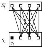
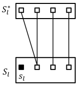
The algorithm allows at most $\rho$ points to be swapped. To satisfy this condition, we consider the following two cases to construct swap operations (cf. Figure 1 for $\rho=3$).

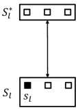
Case 1

(cf. Figure 1(a)). For each $l$ with $|S_{l}|=|S^{*}_{l}|\leq\rho$, we consider the pair $(S_{l},S^{*}_{l})$. Let ${\hat{S}^{*}_{l}}:=\{\hat{s}^{*}|s^{*}\in S^{*}_{l}\}$. W.l.o.g., we assume that ${\hat{S}^{*}_{l}}\subseteq{\mathcal{X}}\setminus S$. For $k$-MedP, we consider the swap$(S_{l},S^{*}_{l})$; for $k$-MeaP, we consider the swap$(S_{l},{\hat{S}^{*}_{l}})$. Utilizing these swap operations, we obtain the following result.

Lemma 3.2.

If $|S_{l}|=|S^{*}_{l}|\leq\rho$, then we have

	$\displaystyle 0$	$\displaystyle\leq$	$\displaystyle\sum\limits_{s\in S_{l}}\sum\limits_{x\in N(s)\cap P^{*}}(p_{x}-{\rm cost}_{c}(x))+\sum\limits_{s\in S_{l}}\sum\limits_{x\in N(s)\setminus P^{*}}\left(d(\phi({\rm cent}_{{\mathcal{C}}}(N^{*}_{q}(s^{*}_{x}))),x)-{\rm cost}_{c}(x)\right)+$		(6)
			$\displaystyle\sum\limits_{s^{*}\in S_{l}^{*}}\sum\limits_{x\in N^{*}(s^{*})\setminus P}({\rm cost}_{c}^{*}(x)-{\rm cost}_{c}(x))+\sum\limits_{s^{*}\in S_{l}^{*}}\sum\limits_{x\in N^{*}(s^{*})\cap P}({\rm cost}_{c}^{*}(x)-p_{x}).$

for $k$-MedP, and

	$\displaystyle 0$	$\displaystyle\leq$	$\displaystyle\sum\limits_{s\in S_{l}}\sum\limits_{x\in N(s)\cap P^{*}}(p_{x}-{\rm cost}_{c}(x))+\sum\limits_{s\in S_{l}}\sum\limits_{x\in N(s)\setminus P^{*}}\left(d^{2}(\phi({\rm cent}_{{\mathcal{C}}}(N^{*}_{q}(s^{*}_{x}))),x)-{\rm cost}_{c}(x)\right)+$		(7)
			$\displaystyle\sum\limits_{s^{*}\in S_{l}^{*}}\sum\limits_{x\in N^{*}(s^{*})\setminus P}((1+{\hat{\varepsilon}}){\rm cost}_{c}^{*}(x)-{\rm cost}_{c}(x))+\sum\limits_{s^{*}\in S_{l}^{*}}\sum\limits_{x\in N^{*}(s^{*})\cap P}((1+{\hat{\varepsilon}}){\rm cost}_{c}^{*}(x)-p_{x}).$

for $k$-MeaP.

Case 2

(cf. Figure 1(b)). For each $l$ with $|S_{l}|=|S^{*}_{l}|=m_{l}>\rho$, we consider $(m_{l}-1)m_{l}$ pairs $(s,s^{*})$ with $s\in S_{l}\backslash\{s_{l}\}$ and $s^{*}\in S^{*}_{l}$. For $k$-MedP, we consider the swap$(s,s^{*})$; for $k$-MeaP, we consider the swap$(s,{\hat{s}^{*}})$. Utilizing these swap operations, we obtain the following result.

Lemma 3.3.

For any $s\in S_{l}\backslash\{s_{l}\}$ and $s^{*}\in S^{*}_{l}$, we have

	$\displaystyle 0$	$\displaystyle\leq$	$\displaystyle\sum\limits_{x\in N(s)\cap P^{*}}(p_{x}-{\rm cost}_{c}(x))+\sum\limits_{x\in N(s)\setminus P^{*}}\left(d(\phi({\rm cent}_{{\mathcal{C}}}(N^{*}_{q}(s^{*}_{x}))),x)-{\rm cost}_{c}(x)\right)+$		(8)
			$\displaystyle\sum\limits_{x\in N^{*}(s^{*})\setminus P}({\rm cost}_{c}^{*}(x)-{\rm cost}_{c}(x))+\sum\limits_{x\in N^{*}(s^{*})\cap P}({\rm cost}_{c}^{*}(x)-p_{x})$

for $k$-MedP, and

	$\displaystyle 0$	$\displaystyle\leq$	$\displaystyle\sum\limits_{x\in N(s)\cap P^{*}}(p_{x}-{\rm cost}_{c}(x))+\sum\limits_{x\in N(s)\setminus P^{*}}\left(d^{2}(\phi({\rm cent}_{{\mathcal{C}}}(N^{*}_{q}(s^{*}_{x}))),x)-{\rm cost}_{c}(x)\right)+$		(9)
			$\displaystyle\sum\limits_{x\in N^{*}(s^{*})\setminus P}((1+{\hat{\varepsilon}}){\rm cost}_{c}^{*}(x)-{\rm cost}_{c}(x))+\sum\limits_{x\in N^{*}(s^{*})\cap P}((1+{\hat{\varepsilon}}){\rm cost}_{c}^{*}(x)-p_{x})$

for $k$-MeaP.

References

- Ahmadian et al. (2017) Ahmadian S, Norouzi-Fard A, Svensson O, Ward J (2017) Better guarantees for k-means and euclidean k-median by primal-dual algorithms. Proceedings of the 58th Annual Symposium on Foundations of Computer Science, 61–72 (IEEE).
- Arora et al. (1998) Arora S, Raghavan P, Rao S (1998) Approximation schemes for euclidean k-medians and related problems. Proceedings of the 30th Annual ACM Symposium on Theory of Computing, 106–113.
- Arya et al. (2004) Arya V, Garg N, Khandekar R, Meyerson A, Munagala K, Pandit V (2004) Local search heuristics for k-median and facility location problems. SIAM Journal on Computing 33(3):544–562.
- Bernstein et al. (2019) Bernstein F, Modaresi S, Sauré D (2019) A dynamic clustering approach to data-driven assortment personalization. Management Science 65(5):2095–2115.
- Borgwardt and Happach (2019) Borgwardt S, Happach F (2019) Good clusterings have large volume. Operations Research 67(1):215–231.
- Byrka et al. (2014) Byrka J, Pensyl T, Rybicki B, Srinivasan A, Trinh K (2017) An improved approximation for k-median, and positive correlation in budgeted optimization. ACM Transactions on Algorithms 13(2):23:1–23:31.
- Charikar et al. (2002) Charikar M, Guha S, Tardos É, Shmoys DB (2002) A constant-factor approximation algorithm for the k-median problem. Journal of Computer and System Sciencess 65(1):129–149.
- Charikar et al. (2001) Charikar M, Khuller S, Mount DM, Narasimhan G (2001) Algorithms for facility location problems with outliers. Proceedings of the 12th Annual ACM-SIAM Symposium on Discrete Algorithms, 642–651 (Society for Industrial and Applied Mathematics).
- Charikar and Li (2012) Charikar M, Li S (2012) A dependent lp-rounding approach for the k-median problem. International Colloquium on Automata, Languages, and Programming, 194–205 (Springer).
- Chen (2008) Chen K (2008) A constant factor approximation algorithm for k-median clustering with outliers. Proceedings of the 19th Annual ACM-SIAM Symposium on Discrete Algorithms, 826–835.
- Cohen-Addad and Karthik (2019) Cohen-Addad V, Karthik C (2019) Inapproximability of clustering in lp metrics. Proceedings of the 60th Annual Symposium on Foundations of Computer Science, 519–539 (IEEE).
- Cohen-Addad et al. (2019) Cohen-Addad V, Klein PN, Mathieu C (2019) Local search yields approximation schemes for k-means and k-median in euclidean and minor-free metrics. SIAM Journal on Computing 48(2):644–667.
- Feng et al. (2019) Feng Q, Zhang Z, Shi F, Wang J (2019) An improved approximation algorithm for the k-means problem with penalties. Proceedings of the 2nd Annual International Workshop on Frontiers in Algorithmics, 170–181 (Springer).
- Friggstad et al. (2019a) Friggstad Z, Khodamoradi K, Rezapour M, Salavatipour MR (2019a) Approximation schemes for clustering with outliers. ACM Transactions on Algorithms 15(2):1–26.
- Friggstad et al. (2019b) Friggstad Z, Rezapour M, Salavatipour MR (2019b) Local search yields a ptas for k-means in doubling metrics. SIAM Journal on Computing 48(2):452–480.
- Gupta et al. (2017) Gupta S, Kumar R, Lu K, Moseley B, Vassilvitskii S (2017) Local search methods for k-means with outliers. Proceedings of the 43rd International Conference on Very Large Data Bases 10(7):757–768.
- Hajiaghayi et al. (2012) Hajiaghayi M, Khandekar R, Kortsarz G (2012) Local search algorithms for the red-blue median problem. Algorithmica 63(4):795–814.
- Hochbaum and Liu (2018) Hochbaum DS, Liu S (2018) Adjacency-clustering and its application for yield prediction in integrated circuit manufacturing. Operations Research 66(6):1571–1585.
- Jain et al. (2003) Jain K, Mahdian M, Markakis E, Saberi A, Vazirani VV (2003) Greedy facility location algorithms analyzed using dual fitting with factor-revealing LP. Journal of the ACM 50(6):795–824.
- Jain and Vazirani (2001) Jain K, Vazirani VV (2001) Approximation algorithms for metric facility location and k-median problems using the primal-dual schema and lagrangian relaxation. Journal of the ACM 48(2):274–296.
- Kanungo et al. (2004) Kanungo T, Mount DM, Netanyahu NS, Piatko CD, Silverman R, Wu AY (2004) A local search approximation algorithm for k-means clustering. Computational Geometry 28(2-3):89–112.
- Korupolu et al. (2000) Korupolu MR, Plaxton CG, Rajaraman R (2000) Analysis of a local search heuristic for facility location problems. Journal of Algorithms 37(1):146–188.
- Krishnaswamy et al. (2018) Krishnaswamy R, Li S, Sandeep S (2018) Constant approximation for k-median and k-means with outliers via iterative rounding. Proceedings of the 50th Annual ACM SIGACT Symposium on Theory of Computing, 646–659.
- Li (2013) Li S (2013) A 1.488 approximation algorithm for the uncapacitated facility location problem. Information and Computation 222:45–58.
- Li and Svensson (2016) Li S, Svensson O (2016) Approximating k-median via pseudo-approximation. SIAM Journal on Computing 45(2):530–547.
- Li et al. (2013) Li Y, Shu J, Wang X, Xiu N, Xu D, Zhang J (2013) Approximation algorithms for integrated distribution network design problems. INFORMS Journal on Computing 25(3):572–584.
- Lloyd (1982) Lloyd S (1982) Least squares quantization in pcm. IEEE Transactions on Information Theory 28(2):129–137.
- Lu and Wedig (2013) Lu SF, Wedig GJ (2013) Clustering, agency costs and operating efficiency: Evidence from nursing home chains. Management Science 59(3):677–694.
- Mahdian et al. (2006) Mahdian M, Ye Y, Zhang J (2006) Approximation algorithms for metric facility location problems. SIAM Journal on Computing 36(2):411–432.
- Makarychev et al. (2016) Makarychev K, Makarychev Y, Sviridenko M, Ward J (2016) A bi-criteria approximation algorithm for k-means. Proceedings of the 19th International Workshop on Approximation Algorithms for Combinatorial Optimization Problems (APPROX), and the 20th International Workshop on Randomization and Computation (RANDOM), 14:1–14:20 (Schloss Dagstuhl-Leibniz-Zentrum fuer Informatik).
- Matoušek (2000) Matoušek J (2000) On approximate geometric k-clustering. Discrete & Computational Geometry 24(1):61–84.
- Ni et al. (2020) Ni W, Shu J, Song M, Xu D, Zhang K (2020) A branch-and-price algorithm for facility location with general facility cost functions. INFORMS Journal on Computing URL http://dx.doi.org/10.1287/ijoc.2019.0921.
- Wang et al. (2015) Wang Y, Xu D, Du D, Wu C (2015) Local search algorithms for k-median and k-facility location problems with linear penalties. Proceedings of the 9th Annual International Conference on Combinatorial Optimization and Applications, 60–71 (Springer).
- Wu et al. (2018) Wu C, Du D, Xu D (2018) An approximation algorithm for the k-median problem with uniform penalties via pseudo-solution. Theoretical Computer Science 749:80–92.
- Zhang et al. (2019) Zhang D, Hao C, Wu C, Xu D, Zhang Z (2019) Local search approximation algorithms for the k-means problem with penalties. Journal of Combinatorial Optimization 37(2):439–453.
- Zhang (2007) Zhang P (2007) A new approximation algorithm for the k-facility location problem. Theoretical Computer Science 384(1):126–135.