Over-Approximation of Fluid Models
Abstract
Fluid models are a popular formalism in the quantitative modeling of biochemical systems and analytical performance models. The main idea is to approximate a large-scale Markov chain by a compact set of ordinary differential equations (ODEs). Even though it is often crucial for a fluid model under study to satisfy some given properties, a formal verification is usually challenging. This is because parameters are often not known precisely due to finite-precision measurements and stochastic noise. In this paper, we present a novel technique that allows one to efficiently compute formal bounds on the reachable set of time-varying nonlinear ODE systems that are subject to uncertainty. To this end, we a) relate the reachable set of a nonlinear fluid model to a family of inhomogeneous continuous time Markov decision processes and b) provide optimal and suboptimal solutions for the family by relying on optimal control theory. The proposed technique is efficient and can be expected to provide tight bounds. We demonstrate its potential by comparing it with a state-of-the-art over-approximation approach.
Index Terms:
Nonlinear systems, Uncertain systems, Markov processes, Optimal controlI Introduction
In the last decades, fluid (or mean-field) models underlying biochemical and computer systems have gained a lot of momentum. Possible examples are chemical reaction networks [1], optical switches [2] and layered queueing networks [3]. The main idea is to approximate the original stochastic model which is usually given in terms of a large-scale continuous time Markov chain (CTMC) by means of a compact system of ordinary differential equations (ODEs). When the number of agents (molecules, jobs, nodes etc.) present in the system tends to infinity, the simulation runs of a suitably scaled version of the CTMC can be shown to converge in probability to the deterministic solution of the underlying fluid model [4, 5]. The law of mass action from chemistry [6], for instance, has been shown to be the fluid model of a CTMC semantics stated on the molecule level [4].
Unfortunately, a precise parameterization of a fluid model is often not possible due to finite-precision measurements or stochastic noise [7, 8]. Hence, in order to verify that a nonlinear fluid model satisfies some given property in the presence of parameter functions that are subject to uncertainty, it becomes necessary to estimate the reachable set. This is because a finite set of possible ODE solutions (i.e., a proper subset of the reachable set) can only be used establish the presence of property violations but does not suffice to exclude their existence in general [9, 10]. Another reason is that closed-form expressions for reachable sets of nonlinear ODE systems are not known in general [11].
The estimation of reachable sets of continuous ODE systems is of crucial importance in the field of control engineering and has received a lot of attention over the decades. Linear ODE systems with uncertainties (alternatively, disturbances) are well-understood because in this case the reachable set can be shown to be convex. The situation where also matrix coefficients are uncertain [12], however, is more challenging than the standard control theoretical setting of additive uncertainties [13, 14, 15, 16]. Bounding the reachable set of nonlinear ODE systems is more difficult and there is a number of different techniques which complement each other. The abstraction approach approximates a nonlinear ODE system locally by an affine mapping [17, 18, 19] or a multivariate polynomial [20, 21]. The error can then be estimated using Taylor approximation and interval arithmetic [19, 22]. While abstraction techniques can cover many practical models, in general it is computationally prohibitive to obtain tight over-approximations for larger nonlinear systems [19, 23]. Lyapunov-like functions [9, 24, 25, 26, 27] known from the stability theory of ODE systems provide an alternative to abstraction techniques. Despite the fact that they often lead to tight bounds, their automatic computation is only possible in special cases [26]. In [28, 29, 30] it has been observed that over-approximation can be encoded as an optimal control problem. While theoretically appealing, the approach relies on the Hamilton-Jacobi equation, a partial differential equation which can only be solved for dynamical systems with few variables [31]. In a similar vein of research, [7, 32] used the necessary optimality conditions of Pontryagin’s principle [31] to derive heuristic estimations on reachable sets of nonlinear ODE systems.
Contributions. In the present paper, we introduce an over-approximation technique for the reachable sets of fluid models. The main idea is to exploit the fact that nonlinear fluid models can be related to the linear Kolmogorov equations of CTMCs. More specifically, the technical novelty of the present work is to prove that a nonlinear fluid model can be over-approximated by solving a family inhomogeneous continuous time Markov decision processes (ICTMDPs) [33] with continuous action spaces and; to show that the family of ICTMDPs can be solved efficiently by modifying the strict version of Pontryagin’s principle [34] which is sufficient for optimality. This allows one to estimate the reachable set of an, in general, nonlinear ODE system by studying the reachable sets of a family of linear ODE systems.
For nonlinear fluid models, the proposed approach a) is efficient; b) induces bounds that can be expected to be tight and; c) allows for an algorithmic treatment in the case where the ODE system is given by multivariate polynomials, thus covering in particular biochemical models. A comparison with the state-of-the-art tool for reachability analysis CORA [35] in the context of the well-known SIRS model from epidemiology [7] confirms the potential of the proposed technique.
Related work on CTMDPs. With efficient solution techniques dating back to the sixties, CTMDPs [33] belong to one of the best studied classes of optimization problems. While there exists a large body of literature on homogeneous CTMDPs, however, much less is known about the inhomogeneous case. Moreover, most works on CTMDPs interpret controls as policies, meaning that only a subclass of uncertainties is admissible [36, Section 8.3]. Additionally, the cost function of interest is often either the discounted or the average cost [33] which cannot be used for the over-approximation of Kolmogorov equations. To the best of our knowledge, the only work which has studied the case of inhomogeneous CTMDPs featuring continuous action spaces and time dependent policies with respect to a cost which can be used for over-approximation is [37]. In this work, three concrete queueing systems were analyzed using Pontryagin’s principle [31]. For each of the three models, the underlying necessary conditions were shown to be already sufficient for optimality.
Paper outline. Section II provides a high-level discussion of our approach using a concrete example. Section III continues by introducing agent networks, a rich class of ODE systems that can be covered by our technique. In Section IV we first relate the reachable set of the original nonlinear ODE system underlying an agent network to the solution of a family of ICTMDPs. Afterwards, we present in Sections IV-A–IV-D an efficient solution approach to ICTMDPs. Section V compares a prototype implementation of the approach with CORA, while Section VI discusses how the approach complements existing approximation techniques. Section VII concludes the paper.
Notation. For nonempty sets and , let denote the set of all functions from to . Note that elements of can be interpreted as vectors with values in and coordinates in . We write for whenever for all . The equality of two functions and , instead, is denoted by . By we refer to the finite set of (agent) states; elements of the reachable set of an ODE system are called concentrations instead. The derivative with respect to time of a function is denoted by . Instead, denotes the characteristic function.
II The Main Idea in a Nutshell
We first discuss the problem and the proposed solution on the example of the SIRS model from epidemiology [38] that is given by the nonlinear ODE system
where and refers to the concentration of susceptible, infected and recovered agents, respectively, and denotes the positive time-varying recovery rate parameter. We are interested in the case where the parameter function is uncertain. More specifically, we assume that , where is a known function resembling the nominal (or average) recovery parameter function, while is an unknown uncertainty which satisfies for some known function . With this, the above ODE system rewrites to
| (1) | ||||
The nominal solution corresponds to the case where , i.e., when . In practice, nominal parameter functions arise from finite-precision measurements, average behavior etc., while uncertainties account for the precision of measurements, conservative parameter estimations and stochastic noise.
Problem to solve. For a given time horizon , we seek to provide, for each , a superset which contains the reachable set . To this end, we bound the maximal deviation of from the nominal trajectory , i.e., for each , we formally estimate the function
| (2) |
Since , we infer
for all and . With this, it holds that
i.e., can be estimated by bounding the positive function . In what follows, we present a technique addressing this task.
First Step: Decoupling. Since the formal estimation of nonlinear dynamical systems is difficult, we relate the solution of (1) to that of a special linear ODE system. More specifically, we relate (1) to the linear Kolmogorov equations of a suitable CTMC. To this end, we first note that (1) is induced by the law of mass action [39] and the chemical reactions
| (3) |
The first reaction of (3) states that an infected agent can infect a susceptible one, while the second reaction implies that an infected agent eventually recovers. Instead, the third reaction expresses the fact that a recovered agent eventually loses its immunity and becomes susceptible again.
Apart from inducing the ODE system (1), the chemical reactions (3) induce also a probabilistic model. Intuitively, given a large group of agents interacting according to (3), the stochastic behavior of a single agent in the group is given in terms of a CTMC with the states such that at time the transition rate
| (4) | ||||
The transition rate from state into state accounts for the fact that the probability of being infected is directly proportional to the concentration of infected agents.
The transition rates provided above imply that the transient probabilities of the CTMC satisfy the Kolmogorov equations
| (5) | ||||
where , and denotes the probability that the fixed agent is susceptible, infected and recovered at time , respectively.
We now make the pivotal observation that the solution of (5) with the initial condition given by is also a solution of (1), i.e., . (To see this, replace each with in (5).) Hence, if we are given , the nonlinear ODE system (1) can be expressed in terms of the linear Kolmogorov equations (5).
Unfortunately, we cannot use (5) directly to estimate from (2) because of the term . We tackle this problem by replacing by , where is the nominal trajectory of (1) in the case of and is a new uncertainty function that satisfies for some positive function . This yields the linear ODE system
| (6) | ||||
The key observation is that for any , the uncertainty induces a solution of (6) which coincides with the solution of (5), meaning that whenever .
Moreover, (6) is a linear ODE system that is decoupled from (1). Thus, instead of considering the maximal deviation of from , , the above discussion motivates to focus on the maximal deviation of from , i.e.,
where is a positive function, and denotes the nominal solution of (6) when and .
Intuitively, takes a guess for as input and provides the new guess for . Our goal is to find an that satisfies for all and (or for short). This is because is a guess for a bound on , while implies that is bounded by whenever itself is bounded by . Building on this intuition, we will prove that implies and provide an algorithm that computes, whenever possible, the smallest such positive function .
Second Step: Approximation of Kolmogorov equations. The above discussion shows that an estimation of requires one to evaluate the function . Thanks to the fact that (6) arises from (5) by decoupling, it can be seen that (6) describes the Kolmogorov equations of a CTMC with time-varying uncertain transition rates that are not coupled to the ODE system (1). This, in turn, allows one to compute any value of by solving a family of tractable optimization problems. More specifically, the value can be computed by determining two uncertainty functions and such that
| (7) |
with and . By interpreting the uncertainty functions and as optimal controls, (7) defines an optimal control problem with cost .
A major result of the paper shows that uncertainty functions and can be efficiently computed by relying on a strict version of Pontryagin’s principle which is sufficient for optimality. Apart from solving (7) exactly, this allows one to devise an efficient procedure for the formal estimation of whose bounds can be expected to be tight.
III Technical Preliminaries
In this section, we introduce agent networks (ANs), a class of nonlinear ODE systems to which our over-approximation technique can be applied. ANs are, essentially, chemical reactions networks whose reaction rate functions are not restricted to the law of mass action. The distinctive feature of ANs is that their dynamics can be related to the linear Kolmogorov equations of CTMCs.
Definition 1.
An agent network (AN) is a triple of a finite set of states , parameters and reaction rate functions . Each reaction rate function
-
•
describes the rate at which reaction occurs;
-
•
takes concentration and parameter vectors and , respectively;
-
•
is accompanied by a multiset of atomic transitions of the form , where describes an agent in state interacting and changing state to .
From a multiset , we can extract two integer valued -vectors and , counting how many agents in each state are transformed during a reaction (respectively produced and consumed). Specifically, for each , let be such that
With these vectors, we can express the -th reaction in the chemical reaction style [4] as follows:
| (8) |
We next introduce the ODE semantics of an AN.
Definition 2.
For a given AN , a continuous parameter function and a piecewise continuous function with with , let
denote the set of admissible uncertainties. Then, the reachable set of with respect to is given by the solution set , where solves
| (9) | ||||
for all . The reachable set at time is given by .
The following example demonstrates Definition 1 and 2 in the context of the SIRS model from Section II. In particular, we remark the following.
Remark 1.
Throughout the paper, the SIRS model from Section II is used to explain definitions and statements. All example environments refer to it.
Example 1.
In the following, we assume that an AN is accompanied by a finite time horizon , a positive initial condition and a Lipschitz continuous parameter function . Moreover, we require that each function
-
is analytic in and linear in , i.e., it holds that ;
-
satisfies whenever and , where is as in (8).
Condition enforces the existence of a unique solution (9) and allows us to apply Pontryagin’s principle in Section IV-A, while condition says essentially that the -th reaction (8) can only take place when all its reactants have a positive concentration.
We wish to point out that and can be easily checked because analytic functions are closed under summation, multiplication and composition. Additionally, functions often enjoy a simple form in practical models (in the case of biochemistry, for instance, they are given in terms of monomials).
With and in place, the following can be proven.
Proposition 1.
In the case and hold true, (9) admits a unique solution on for any uncertainty function . Moreover, there exists an such that for all and .
Proof.
Local existence and uniqueness are ensured by [31, Section 3.3.1]. Let us define ,
for all and let denote the vector with if and when . With this, implies for all and that
because the function is nonnegative. Hence, , thus implying that for all . We next show that is positive on . To this end, let us assume towards a contradiction that there is such that for some . Thanks to the continuity of , we may assume without loss of generality that is positive on . With , it holds that . There exists a sufficiently small interval on which Euler’s sequence given by , where and , converges to a local solution of [40]. By construction, the sequence has to converge to a positive function on as . However, thanks to , implies for all regardless how small is, thus yielding a contradiction. Moreover, since and for all , we also infer the existence of on the whole . ∎
It can be seen that atomic transitions enforce conservation of mass, i.e., the creation and destruction of agents is ruled out at the first sight. This problem, however, can be alleviated by the introduction of artificial agent states, see [41].
Kolmogorov Equations of Agent Networks. Thanks to the fact that the dynamics of an AN arise from atomic transitions, it is possible to define a CTMC underlying a given AN which Kolmogorov equations are closely connected to the ODE system (9).
Definition 3.
For a given AN , define
for all with , and . Then, the coupled CTMC underlying and has state space and its transition rate from state into state at time is . The coupled Kolmogorov equations of are
| (11) | ||||
In the context of the SIRS example, Definition 3 gives rise to the transition rates (4), the uncertainty function and the Kolmogorov equations (5). This is because the atomic transitions , and appear only in , and of Example 1, respectively, thus yielding
where and are as in Example 1.
The next pivotal observation establishes a relation between the ODE system (9) and the Kolmogorov equations (11).
Proposition 2.
Proof.
In the context of the SIRS example, Proposition 2 states that the solutions of (1) and (5) coincide whenever .
It is possible to prove that (9) and (11) are the fluid limits of certain CTMC sequences in the case where and the number of agents in the system tends to infinity, see [5, 41, 42] for details. We will not elaborate on this relation further because it is not required for the understanding of our over-approximation technique.
IV Over-Approximation Technique
As anticipated in Section II and III, we estimate the reachable set of an AN with respect to an uncertainty set , i.e., we bound for each . To this end, we study the maximal deviation from the nominal trajectory attainable across .
Definition 4.
For a given AN with uncertainty set , the maximal deviation at time of (9) from is
| (13) |
with and . With this, it holds that
By Proposition 2, any trajectory of (9) coincides with the trajectory of (11) if . Even though this allows one to relate the reachable set of a nonlinear system to that of a linear one, the transition rates of the coupled CTMC depend on . We address this by decoupling the transition rates of the coupled CTMC from .
Definition 5.
In the context of the AN from Example 1, the decoupled Kolmogorov equations (14) are given by (6) with . This is because the transition rates of the decoupled CTMC are
| (15) | ||||
A direct comparison with the transition rates of the coupled CTMC given in (4) reveals that the original transition rate from into , , is replaced with .
Remark 2.
Note that can be efficiently computed using a numerical ODE solver and by setting in (9) to zero.
Proposition 3.
Assume that . Then, for any , there exists some such that the solution of (14) subject to the initial condition satisfies for all .
Proof.
To provide an estimation of using the Kolmogorov equations (14), we next define as the maximal deviation from the nominal trajectory that can be attained across the uncertainties and .
Definition 6.
For a piecewise continuous function , let be given by
denotes the maximal deviation of from , where arises from in (14) if .
As discussed in Section II, the goal is to find a positive function such that . This ensures that for any and implies, as stated in the next important result, that .
Theorem 1.
If , then .
Remark 3.
A direct consequence of Theorem 1 is that a fixed point of estimates from above whenever .
The next result describes an algorithm for the computation of the least fixed point .
Theorem 2.
Fix some small and set
for all . If such that , then is the smallest fixed point of which satisfies .
Proof.
Obviously, is monotonic increasing, i.e., implies . With this, Kleene’s fixed point theorem yields the claim. ∎
Note that the computation of the sequence can be terminated if is violated because in such case no bound can be obtained.
IV-A Optimal Solutions for inhomogeneous CTMDPs
In each step of the fixed point iteration from Theorem 2, a new value of has to be computed. To this end, for any and , we have to
| (16) |
While the solution of such optimization problems is particulary challenging in the case of nonlinear dynamics, time-varying systems such as (16) are easier to come by. This is because (16) is a linear system with additive and multiplicative uncertainties. More formally, (16) is linear in concentrations variables if the parameter variables are fixed and linear in parameter variables when the concentration variables are fixed.
Remark 4.
For the benefit of presentation, we write in that what follows instead of , where and for all and , respectively. Moreover, we recall that a solution of a differential inclusion is any absolutely continuous function which satisfies almost everywhere.
We solve (16) by modifying the strict version of Pontryagin’s principle [34] which is sufficient for optimality. Our modification of [34] is less general than the original because it is stated for CTMCs but it makes weaker assumptions (the concavity of is required on positive values only).
Theorem 3.
For any , let and assume that, for any and , the function
is concave on . Then, any solution of the differential inclusion
subject to (12) and () minimizes (maximizes) the value of .
Proof.
The proof follows the argumentation of [34]. Fix some and and let denote the solution underlying . Note that it suffices to consider continuous uncertainties because standard results from ODE theory and functional analysis ensure that the maximal value can be attained by continuous uncertainties, that is
where and . For the ease of notation, let , and denote a solution of the differential inclusion and set
where denotes the dot product. Thanks to the fact that , integration by parts yields
With this, it holds that
where the first inequality is implied by the concavity of , while the second inequality follows from the definition of and the choice of . In the case where we seek to maximize the value of , we note that yields . Since the case of minimization is similar, the proof is complete. ∎
We next identify structural conditions on which can be easily checked and that imply the technical requirement of concavity of Theorem 3.
-
(A1)
For any and , there exist Lipschitz continuous such that the transition rate function from Definition 3 satisfies
for all and .
-
(A2)
For each , there exist unique such that implies , and .
Assumption (A1) requires, essentially, the transition rate functions to be linear in the uncertainties, while (A2) forbids the same uncertainty to affect more than one transition of the decoupled CTMC .
The next example demonstrates that our running example satisfies condition (A1) and (A2).
Example 2.
The following crucial theorem can be shown in the presence of . We wish to stress that the result can be also applied to an ICTMDP which is not induced by an AN.
Theorem 4.
Proof.
In the following, we verify that a solution of (18)-(20) is a solution of the differential inclusion from Theorem 3. To this end, we first observe that
Hence, we infer that
This and Theorem 3 show that an optimal control must satisfy (4). Moreover, it implies that
for all and , thus yielding linearity (and thus also concavity) of on . The last statement follows by noting that
for all . ∎
We wish to stress that Theorem 4 ensures that any solution of the differential inclusion (18), (4) induces an ODE solution of (20) such that , where denotes the solution of (16). This stands in stark contrast to the standard version of Pontryagin’s principle [31] which provides only necessary conditions for optimality, meaning that the value arising from the standard version [31] may fail to satisfy .
Solving a differential inclusion is a challenging task and requires one to assume in practice that it does not exhibit sliding or gazing modes [43, 44]. Fortunately, the next crucial results states that it is possible to obtain a specific solution of the differential inclusion (18), (4) by solving a Lipschitz continuous ODE system.
Theorem 5.
Proof.
Let denote the drift of the ODE system (18) which underlies (21), that is
with being as in (21). Fix some and pick further two sequences and in which converge both to as . We first show that as . To this end, it suffices to observe that any with implies (recall that yields ). Hence, it holds that
as . This shows the continuity of . To see also the Lipschitzianity, define
for each with . Note that if and only if because whenever . Moreover, for any , is Lipschitz continuous on any bounded subset of because and are Lipschitz continuous on . This shows that is Lipschitz continuous on any bounded subset of . With this, the continuity of implies that is Lipschitz continuous on any bounded subset of . ∎
In the remainder of the paper, we replace (4) by (21). Theorem 5 ensures that (18) admits a unique solution and that the underlying optimal uncertainty induces the minimal (maximal) value via (21) and (20).
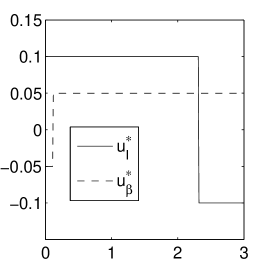

Example 3.
We have seen in Example 2 that our running example satisfies the requirements of Theorem 4. In particular, if , then (18) and (21) rewrite to
| (22) | ||||
and
respectively. The minimal value of, say, can be obtained as follows. First, solve the ODE system (22) where the boundary condition is given by and . Afterwards, using the obtained solution , solve the ODE system (20) using the controls and . A possible solution is visualized in Figure 1.
While Theorem 5 solves the problem from a theoretical point of view, it has to be noted that a numerical solution of the Lipschitz continuous ODE system (4), (21) is an approximation of the true solution . Hence, for any with , the computation of the optimal uncertainty may be hindered by the numerical errors underlying the ODE solver. The next crucial result addresses this issue by stating that, essentially, for each such the choice of is not important.
Theorem 6.
Proof.
With , and , let the function be such that whenever . Using the same notation as in the proof of Theorem 3, we infer in the case when the following:
where the first identity holds true because is linear (see proof of Theorem 4), while the other identities follow as in the proof of Theorem 3. The above calculation yields
where the second equality follows from the proof of Theorem 4. ∎
The above theorem states, essentially, that the choice of is irrelevant at all time points with . Hence, an uncertainty that is induced by a numerical solution of (18) can be used to solve (16).
We end the section by mentioning the following generalization of Theorem 4.
IV-B Proof of Theorem 1
Armed with Theorem 4 and Theorem 5, we are now in a position to prove Theorem 1 under the assumption that the decoupled CTMC from Definition 5 satisfies (A1) and (A2). The assumption will be dropped in Section IV-C.
Proof of Theorem 1.
Let us assume towards a contradiction that and are positive piecewise constant functions, that is analytic and that there exists an analytic uncertainty function , a time and some such that and for all and . Since , we may assume without loss of generality that . With this, we consider the optimization problem
| (23) |
where is as in (14). Let denote the solution of (23) and set with . Since , we infer . Hence, is an optimal control and Theorem 4 and 5 imply that whenever , where is as in (21), and solves (18) and (21). At the same time, the analyticity of , and implies that is analytic as well [41]. Since and are piecewise constant and none of the can be locally constant (otherwise the in question would be constant on the whole by the identity theorem), we infer that for all . Recall from the proof of Theorem 6 that
| (24) |
and that the Hamiltonian is invariant with respect to the value of when . This, the above discussion and (24) imply that for any uncertainty . As this contradicts , we infer the statement of the theorem in the case where and are piecewise constant and and are analytic. Thanks to the fact that analytic and piecewise constant functions are dense in set of bounded measurable functions on , this suffices the claim. ∎
IV-C Sub-Optimal Solutions for inhomogeneous CTMDPs
It may happen that the decoupled CTMC from Definition 5 violates (A1) or (A2). We next discuss a procedure which allows one to transform a CTMC violating (A1)-(A2) into one which satisfies (A1)-(A2). We convey the main ideas using concrete examples.
The extension of Example 1 discussed next induces a decoupled CTMC which violates (A1).
Example 4.
Consider the agent network given by
where and . Let the time-varying uncertain infection and recovery parameter functions be given by and , respectively, where and . Then, the AN induces the reactions
and the transition rates of the decoupled CTMC from Definition 5 are given by
Since
leads to the nonlinear term , the decoupled CTMC does not satisfy (A1).
The idea is to substitute any nonlinear expression of uncertainties by a new uncertainty that bounds the original nonlinear expression. For instance, in the case of Example 4, we substitute with the new uncertainty and set because .
This motivates the following concept.
Definition 7.
For a family of transition rates is an envelope of the transition rates from Definition 5 if there exist Lipschitz continuous functions , an index set with and a piecewise continuous function such that for all one can pick a so that
for all .
By construction, any envelope satisfies (A1). It may however happen that an envelope does not satisfy (A2). To see this on an example, we extend Example 4 to the multi-class SIRS model [7] in which the overall population of agents is partitioned into classes, thus providing a better picture of the actual spread dynamics [38].
Example 5.
With being the number of classes, the multi-class SIRS agent network is given by the atomic reactions
where . In the case where all rates are subject to uncertainty, the reactions are
| (25) | ||||
The first reaction expresses the fact that a susceptible agent of class may be infected by an infected agent from class . The transition rates of the decoupled CTMC are
The nonlinear terms prevent the decoupled CTMC to satisfy (A1). Similarly to Example 4, we thus consider the envelope
| (26) |
with . Unfortunately, envelope (5) violates (A2) because each is contained in , …, .
We continue by observing that envelope (5) can be transformed into a set of transition rates which satisfies (A1) and (A2). Indeed, if we substitute in each from (5) the uncertainty with , the transition rates
| (27) |
define a CTMC which satisfies (A1) and (A2). This is because every uncertainty function , where and
with and , appears in exactly one transition rate .
This above discussion motivates the following.
Definition 8.
Assume that is an envelope of given by
for all and let be such that violates (A2) for each . Then, the transition rate arises from by substituting each occurrence of in with , where . By setting , the coarsening of is given by .
Remark 6.
The next result states that the coarsening of an envelope of the decoupled CTMC from Definition 5 allows one to estimate from Definition 4.
Theorem 7.
Given the decoupled CTMC from Definition 5, let us assume that is an envelope for . Let further denote the coarsening of as given in Definition 8 and let
| (28) |
denote the Kolmogorov equations underlying the coarsening . Set further and
Then, applying the fixed point iteration algorithm of Theorem 2 to instead of yields a bound on . Moreover, Theorem 4 and Theorem 5 carry over to the extended set of uncertainties and can be used to compute .
Proof.
To see that implies , let , , , , , , and be as in the proof from Section IV-B. Then, it holds that , where solves
and the inequality holds true because the definition of the envelope and the coarsening of an envelope ensure that for any function there exists some function such that
for all . This implies . Moreover, it can be observed that Theorem 4 and Theorem 5 hold for any CTMC which transition rates satisfy (A1) and (A2). Hence, they can be used to compute (just replace the index set with ). This and the definition of the envelope and the coarsening of an envelope ensure the existence of some such that is optimal, i.e., . In the case is piecewise constant for all , the argumentation from Section IV-B leads to the desired contradiction. With this, the density argument from Section IV-B implies that . Since is monotonic increasing, the proof is complete. ∎
It is interesting to note that Theorem 1 allows one to derive bounds on from Definition 4 using any estimation technique that applies to (16). Put different, Theorem 4 and 5 can be replaced, in principle, by any over-approximation technique applicable to time-varying linear systems with uncertain additive and multiplicative uncertainties. Note, however, that the bounds obtained by Theorem 4 and 5 cannot be improved if the decoupled CTMC satisfies (A1)-(A2) and can be expected to be tight even if (A1)-(A2) are violated because Theorem 7 relies on optimal control theory.
IV-D Algorithm
The previous sections gives rise to Algorithm 1 which summarizes all steps of our approximation technique. Apart from line 4 that has to compute an envelope of the transition rates of the decoupled CTMC from Definition 5 (see Definition 7), all steps of Algorithm 1 can be automatized. Indeed, the computation of the coarsening in line 8 is the variable substitution introduced in Definition 8, while in line 11 can be obtained by applying, for any and , Theorem 4 in order to compute the maximal and minimal value of across all .
Computation of an envelope. In the case the reaction rate functions of the agent network are multivariate polynomials as in the case of our running example discussed in Example 1-5, the envelope from line 4 can be efficiently computed by Algorithm 2. This makes our approach particularly suited to models from the field of biochemistry. Note that Algorithm 2 replaces any product of uncertainties by a new uncertainty and bounds it by the maximal value of the replaced product similarly to the discussion following Example 4.
Computation of . We conclude the section by discussing a rigorous and a heuristic implementation of line 11. In the case of the former, one has to combine Theorem 4, 5 and 6 with a verified numerical ODE solver as [45] that provides apart from a numerical solution also an estimation of the underlying numerical error [40]. Additionally to the numerical error, one has to account for the discretization error arising in the computation of , where the idea is to evaluate only at grid points from by computing the maximal and minimal value of from (7) for all and .
The following result can be proven.
Theorem 8.
For any positive function and , the function can be approximated with precision by solving ODE systems of size , where
| (29) |
and denotes the Kolmogorov equations underlying the transition rates from Algorithm 1.
| CORA | Algorithm 1 for | Algorithm 1 for | ||||||
|---|---|---|---|---|---|---|---|---|
| Run time | Run time | Run time | ||||||
| 1 | 3 | 3 | 0m | 0.187 | 2m | 0.158 | 3m | 0.163 |
| 2 | 6 | 8 | 1m | 0.238 | 4m | 0.124 | 6m | 0.130 |
| 3 | 9 | 15 | 1m | 0.296 | 8m | 0.109 | 11m | 0.116 |
| 4 | 12 | 24 | 2m | 0.377 | 13m | 0.100 | 17m | 0.109 |
| 5 | 15 | 35 | 4m | 0.494 | 18m | 0.096 | 24m | 0.103 |
| 6 | 18 | 48 | 5m | 0.694 | 19m | 0.091 | 29m | 0.101 |
| 7 | 21 | 63 | — | — | 30m | 0.091 | 43m | 0.094 |
| 8 | 24 | 80 | — | — | 40m | 0.084 | 53m | 0.096 |
| 9 | 27 | 99 | — | — | 50m | 0.087 | 65m | 0.096 |
| 10 | 30 | 120 | — | — | 61m | 0.091 | 78m | 0.095 |
Proof.
We prove that we need to solve instances of (18) and (20), respectively. To this end, we first note that from (7) is absolutely continuous and has derivative almost everywhere. This yields
for any . Since for all , we infer that . This implies that we miss the actual value of by at most if we compute the maximal and minimal value of for all and . With this, we note that implies which, in turn, induces grid points. Since we need to compute the minimum and maximum value of for all and , this yields the claim. ∎
Apart from the rigorous implementation, our approach allows for a heuristic implementation. Here, instead of using a verified numerical ODE solver, one invokes a standard ODE solver in which the numerical error is minimized heuristically by varying the integration step size [40]. Similarly, one accounts heuristically for the discretization underlying by gradually refining an initially coarse discretization of until the approximations of are reasonably close.
We wish to point out that both implementations naturally apply to parallelization because each single ODE system can be solved independently from the others.
V Numerical Evaluation
In this section we study the potential of our technique by applying it on the multi-class SIRS model from Section IV-C. To this end, we implemented an experimental prototype of the heuristic version from Section IV-D in Matlab by relying on the (non-verified) numerical ODE solver provided by the Matlab command ode45s. The heuristic implementation was compared with the state-of-the-art reachability analysis tool CORA [35] that covers nonlinear ODE systems with multiplicative uncertainty functions.
All experiments were performed on a 3.2 GHz Intel Core i5 machine with 8 GB of RAM. The Matlab solver ode45s was invoked with its default settings. For CORA, instead, the time step was set to , while the expert settings were chosen as in the nonlinear tank example from the CORA manual [46]. The main findings are as follows.
-
•
The bounds obtained by the heuristic implementation are tight;
-
•
CORA is faster than the heuristic implementation in the case of smaller systems;
-
•
The heuristic implementation scales to models that cannot be covered by CORA.
The above confirms the discussion from Section IV-D concerning the complexity of our approach. Indeed, for smaller ODE systems, our approach is inferior to CORA because of the discretization of the time interval . However, for abstraction approaches such as CORA it is computationally prohibitive to obtain tight over-approximations for larger nonlinear systems in general. Instead, our approach requires to solve ODE systems of size , see Theorem 8. Moreover, at least as far as the heuristic implementation is considered, we were able to obtain tight bounds. In summary, we argue that our technique has the potential to complement state-of-the-art over-approximation approaches.
Multi-class SIRS Model. The global dynamics underlying (25) is given by
| (30) |
where , , are time-varying uncertain functions and for some . The system has ODE variables and uncertainties. As discussed in Section IV-C, the transition rates (IV-C) define a function as in Theorem 7 that can be used to estimate the function underlying (V).
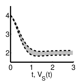
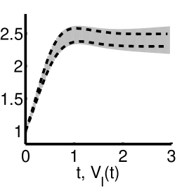
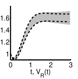
In our experiments, we randomly chose , , and , for all . The time horizon was set to , while all parameters were subject to uncertainties with modulus not higher than , i.e., for all and .
Table I and Figure 2 summarize our findings. With increasing , the tightness of the bounds provided by CORA decreases while the corresponding running times increase. In principle, the tightness can be improved by using stricter parameters (e.g., by decreasing the step size). This, however, increases the time and space requirements. Likewise, the over-approximation of larger models requires more resources in general. On our machine, for instance, or time steps below led to out-of-memory errors. The heuristic implementation of Algorithm 1, instead, scales to larger instances of the running example and provides tight bounds. Indeed, since the from (29) can be chosen as in the case of the ODE system (25), Theorem 8 implies that one has to solve ODE systems of size in order to guarantee that a numerical approximation of from Theorem 7 misses the actual value of by at most . We approximated the values of from Algorithm 1 using discretizations and , where
The run times account for the computation of the sequence from Algorithm 1 with . In agreement with Theorem 8, the running times exhibit a polynomial growth. Moreover, discretizations and induce bounds that are reasonably close.
VI Discussion
While Pontryagin’s principle and its extensions to systems with uncertain parameters have been used in the context of reachability analysis [7, 32], to the best of our knowledge, the principle has not been applied in the context of formal over-approximation of a general class of nonlinear ODE systems. This is because the principle is in general only a necessary condition for optimality, while its strict versions [34, 47] require concavity or convexity which is rarely satisfied by nonlinear ODE models. Additionally, Pontryagin’s principle induces in general a differential inclusion which can only be solved under additional assumptions [43, 44]. The present work addresses those problems by a) approximating the original nonlinear ODE system by a family of linear Kolmogorov equations (14) with multiplicative and additive uncertainties and; by b) showing that each family member can be over-approximated tightly and efficiently using a modified version of the strict version of Pontryagin’s principle [34].
The proposed approach is complementary to existing approximation techniques. Indeed, while it is less efficient than approaches that are based on monotonic systems and differential inequalities [48, 49, 22, 8], it may provide tighter bounds because it relies on optimal control theory. Instead, for approaches based on abstraction [21, 35] and the Hamilton-Jacobi equation [29, 30], in general it becomes computationally prohibitive to obtain tight over-approximations for larger nonlinear systems [19, 23]. Another point worth stressing is that many approaches applicable to nonlinear ODE models assume time-invariant uncertain parameters and uncertain initial conditions, while the present technique focusses on nonlinear ODE systems with time-varying uncertain parameters and fixed initial conditions. Since the proposed approximation technique relies on the availability of a concrete nominal solution, a direct extension to sets of initial conditions seems not to be possible. This notwithstanding we wish stress that it is particulary suited to systems biology where initial concentrations can be measured while reaction rates are often difficult to obtain and may vary with time.
VII Conclusion
In this work we presented an over-approximation technique for nonlinear ODE systems with time-varying uncertain parameters. Our approach provides verifiable bounds in terms of a family of linear Kolmogorov equations with uncertain additive and multiplicative time-varying parameters. To ensure efficient computation and tight estimations, we have established, to the best of our knowledge, a novel efficiently computable solution technique for a class of inhomogeneous continuous time Markov decision processes.
The presented over-approximation technique is efficient and can be expected to provide tight bounds because it relies on optimal control theory and allows for an algorithmic treatment in the case where the ODE system is given by multivariate polynomials. This makes it particularly suited to models from (bio)chemistry.
By comparing our approach with a state-of-the-art over-approximation technique in the context of the multi-class SIRS model from epidemiology [7], we have provided numerical evidence for the potential of our approach. The most pressing line of future work is the development of a tool which provides a rigorous implementation of the technique.
Acknowledgement
The author thanks Mirco Tribastone for helpful discussions. Parts of the work have been conducted when the author was with IMT Lucca. The author is supported by a Lise Meitner Fellowship that is funded by the Austrian Science Fund (FWF) under grant number M 2393-N32 (COCO).
References
- [1] L. Cardelli, A. Csikász-Nagy, N. Dalchau, M. Tribastone, and M. Tschaikowski, “Noise Reduction in Complex Biological Switches.” Scientific reports, 2016.
- [2] B. V. Houdt and L. Bortolussi, “Fluid limit of an asynchronous optical packet switch with shared per link full range wavelength conversion,” in SIGMETRICS, 2012, pp. 113–124.
- [3] M. Tribastone, “A Fluid Model for Layered Queueing Networks,” IEEE Transactions on Software Engineering, vol. 39, no. 6, pp. 744–756, 2013.
- [4] T. G. Kurtz, “The relationship between stochastic and deterministic models for chemical reactions,” The Journal of Chemical Physics, vol. 57, no. 7, pp. 2976–2978, 1972.
- [5] L. Bortolussi, J. Hillston, D. Latella, and M. Massink, “Continuous approximation of collective system behaviour: A tutorial,” Performance Evaluation, vol. 70, no. 5, pp. 317–349, 2013.
- [6] L. Cardelli, M. Tribastone, M. Tschaikowski, and A. Vandin, “Maximal aggregation of polynomial dynamical systems,” Proceedings of the National Academy of Sciences, vol. 114, no. 38, pp. 10 029 –10 034, 2017.
- [7] L. Bortolussi and N. Gast, “Mean Field Approximation of Uncertain Stochastic Models,” in DSN, 2016.
- [8] M. Tschaikowski and M. Tribastone, “Approximate Reduction of Heterogenous Nonlinear Models With Differential Hulls,” IEEE Transactions Automatic Control, vol. 61, no. 4, pp. 1099–1104, 2016.
- [9] S. Prajna, “Barrier certificates for nonlinear model validation,” Automatica, vol. 42, no. 1, pp. 117–126, 2006.
- [10] A. Abate, M. Prandini, J. Lygeros, and S. Sastry, “Probabilistic reachability and safety for controlled discrete time stochastic hybrid systems,” Automatica, vol. 44, no. 11, pp. 2724–2734, 2008.
- [11] G. Lafferriere, G. J. Pappas, and S. Yovine, A New Class of Decidable Hybrid Systems, 1999.
- [12] M. Althoff, C. Le Guernic, and B. H. Krogh, “Reachable Set Computation for Uncertain Time-Varying Linear Systems,” in HSCC, 2011, pp. 93–102.
- [13] A. B. Kurzhanski and P. Varaiya, “Ellipsoidal Techniques for Reachability Analysis,” in HSCC, N. Lynch and B. H. Krogh, Eds., 2000.
- [14] A. Girard, C. Le Guernic, and O. Maler, “Efficient Computation of Reachable Sets of Linear Time-Invariant Systems with Inputs,” in HSCC, 2006.
- [15] A. Girard and C. Le Guernic, “Efficient reachability analysis for linear systems using support functions,” in IFAC, 2008.
- [16] S. Bak and P. S. Duggirala, “HyLAA: A Tool for Computing Simulation-Equivalent Reachability for Linear Systems,” in HSCC, 2017, pp. 173–178.
- [17] E. Asarin, T. Dang, and A. Girard, “Reachability Analysis of Nonlinear Systems Using Conservative Approximation,” in HSCC, 2003.
- [18] A. Donzé and O. Maler, “Systematic Simulation Using Sensitivity Analysis,” in HSCC. Springer, 2007, pp. 174–189.
- [19] M. Althoff, “Reachability Analysis of Nonlinear Systems using Conservative Polynomialization and Non-Convex Sets,” in HSCC, 2013, pp. 173–182.
- [20] M. Berz and K. Makino, “Verified Integration of ODEs and Flows Using Differential Algebraic Methods on High-Order Taylor Models,” Reliable Computing, vol. 4, no. 4, pp. 361–369, 1998.
- [21] X. Chen, E. Ábrahám, and S. Sankaranarayanan, “Flow*: An Analyzer for Non-linear Hybrid Systems,” in CAV, 2013, pp. 258–263.
- [22] J. K. Scott and P. I. Barton, “Bounds on the reachable sets of nonlinear control systems,” Automatica, vol. 49, no. 1, pp. 93 – 100, 2013.
- [23] P. S. Duggirala and M. Viswanathan, “Parsimonious, Simulation Based Verification of Linear Systems,” in CAV, 2016, pp. 477–494.
- [24] D. Angeli, “A Lyapunov approach to incremental stability properties,” IEEE Trans. Automat. Contr., vol. 47, no. 3, pp. 410–421, 2002.
- [25] M. Zamani and R. Majumdar, “A Lyapunov approach in incremental stability,” in CDC, 2011.
- [26] A. Girard and G. J. Pappas, “Approximate bisimulations for nonlinear dynamical systems,” in CDC. IEEE, Jun. 2005, pp. 684–689.
- [27] C. Fan, B. Qi, S. Mitra, M. Viswanathan, and P. S. Duggirala, Automatic Reachability Analysis for Nonlinear Hybrid Models with C2E2, 2016, pp. 531–538.
- [28] A. M. Bayen, E. Crück, and C. J. Tomlin, “Guaranteed overapproximations of unsafe sets for continuous and hybrid systems: Solving the Hamilton-Jacobi equation using viability techniques,” in HSCC, 2002, pp. 90–104.
- [29] J. Lygeros, “On reachability and minimum cost optimal control,” Automatica, vol. 40, no. 6, pp. 917–927, 2004.
- [30] I. M. Mitchell, A. M. Bayen, and C. J. Tomlin, “A time-dependent Hamilton-Jacobi formulation of reachable sets for continuous dynamic games,” IEEE TAC, vol. 50, no. 7, pp. 947–957, 2005.
- [31] D. Liberzon, Calculus of Variations and Optimal Control Theory: A Concise Introduction. Princeton University Press, 2011.
- [32] H. Frankowska, “The Maximum Principle for an Optimal Solution to a Differential Inclusion with End Points Constraints,” SIAM Journal on Control and Optimization, vol. 25, no. 1, pp. 145–157, 1987.
- [33] X. Guo and O. Hernandez-Lerma, Continuous-Time Markov Decision Processes. Springer Verlag, 2009.
- [34] M. I. Kamien and N. L. Schwartz, “Sufficient conditions in optimal control theory,” Journal of Economic Theory, vol. 3, no. 2, pp. 207 – 214, 1971.
- [35] M. Althoff, “An introduction to CORA 2015,” in Proc. of the Workshop on Applied Verification for Continuous and Hybrid Systems, 2015.
- [36] N. B uerle and U. Rieder, Markov Decision Processes with Application to Finance. Springer Verlag, 2011.
- [37] R. C. Hampshire and W. A. Massey, Dynamic Optimization with Applications to Dynamic Rate Queues, ch. Chapter 10, pp. 208–247.
- [38] G. Iacobelli and M. Tribastone, “Lumpability of fluid models with heterogeneous agent types,” in DSN, 2013, pp. 1–11.
- [39] L. Cardelli, M. Tribastone, M. Tschaikowski, and A. Vandin, “Forward and Backward Bisimulations for Chemical Reaction Networks,” in CONCUR, 2015, pp. 226–239.
- [40] C. W. Gear, Numerical Initial Value Problems in Ordinary Differential Equations. Upper Saddle River, NJ, USA: Prentice Hall PTR, 1971.
- [41] L. Bortolussi and J. Hillston, “Model checking single agent behaviours by fluid approximation,” Information and Computation, vol. 242, pp. 183–226, 2015.
- [42] R. Darling and J. Norris, “Differential equation approximations for Markov chains,” Probability Surveys, vol. 5, pp. 37–79, 2008.
- [43] A. Dontchev and F. Lempio, “Difference Methods for Differential Inclusions: A Survey,” SIAM Review, vol. 34, no. 2, pp. 263–294, 1992.
- [44] L. Bortolussi, “Hybrid Limits of Continuous Time Markov Chains,” in QEST, 2011, pp. 3–12.
- [45] O. Bouissou and M. Martel, “GRKLib: a guaranteed Runge-Kutta library,” in GAMM - IMACS SCAN, 2007.
- [46] M. Althoff, “Cora 2016 manual.” [Online]. Available: http://www.i6.in.tum.de/pub/Main/SoftwareCORA/Cora2016Manual.pdf
- [47] V. Azhmyakov and J. Raisch, “Convex control systems and convex optimal control problems with constraints,” IEEE Transactions on Automatic Control, vol. 53, no. 4, pp. 993–998, 2008.
- [48] N. Ramdani, N. Meslem, and Y. Candau, “Reachability of uncertain nonlinear systems using a nonlinear hybridization,” in HSCC, 2008, pp. 415–428.
- [49] ——, “Computing reachable sets for uncertain nonlinear monotone systems,” Nonlinear Analysis: Hybrid Systems, vol. 4, no. 2, pp. 263 – 278, 2010, iFAC World Congress 2008.
![[Uncaptioned image]](https://cdn.awesomepapers.org/papers/c1b54cc4-47d3-4950-8fc6-91fbcbb164dc/Max.jpg) |
Max Tschaikowski is a Lise Meitner Fellow at the Technische Universität Wien, Austria. Prior to it, he was a non-tenure-track Assistant Professor at IMT Lucca, Italy, a Research Fellow at the University of Southampton, UK, and a Research Assistant at the LMU in Munich, Germany. He was awarded a Diplom in mathematics and a Ph.D. in computer science by the LMU in 2010 and 2014, respectively. His research focusses on the construction, reduction and verification of quantitative models. |