This paper was converted on www.awesomepapers.org from LaTeX by an anonymous user.
Want to know more? Visit the Converter page.

PAC-Bayesian Generalization Bounds for
MultiLayer Perceptrons

Xinjie Lan, Xin Guo, Kenneth E. Barner
Department of Electrical and Computer Engineering, University of Delaware
lxjbit@udel.edu
Abstract

We study PAC-Bayesian generalization bounds for Multilayer Perceptrons (MLPs) with the cross entropy loss. Above all, we introduce probabilistic explanations for MLPs in two aspects: (i) MLPs formulate a family of Gibbs distributions, and (ii) minimizing the cross-entropy loss for MLPs is equivalent to Bayesian variational inference, which establish a solid probabilistic foundation for studying PAC-Bayesian bounds on MLPs. Furthermore, based on the Evidence Lower Bound (ELBO), we prove that MLPs with the cross entropy loss inherently guarantee PAC-Bayesian generalization bounds, and minimizing PAC-Bayesian generalization bounds for MLPs is equivalent to maximizing the ELBO. Finally, we validate the proposed PAC-Bayesian generalization bound on benchmark datasets.

1 Introduction

To explain why Deep Neural Networks (DNNs) with Stochastic Gradient Descent (SGD) optimization can achieve impressive generalization performance [15], a generalization bound should satisfy the five criteria: (i) small and non-vacuous [8, 39]; (ii) taking into account SGD optimization because DNNs not incorporate any explicit regularization [1, 13, 21]; (iii) showing the same architecture dependence as the generalization error, e.g., it should become smaller as the architecture of DNNs becomes complex [30, 33, 32]; (iv) showing the same sample size dependence as the generalization error, i.e., it should become smaller as the training sample size becomes larger [29, 30]; and (v) taking into account the statistical variations of samples and labels, especially random labels [38].

PAC-Bayesian theory provides a canonical probabilistic framework for studying generalization bounds [25, 26, 6, 11, 2, 28]. However, due to the extremely complicated architecture of DNNs, most existing works avoid directly formulating the prior distribution of the hypothesis expressed by DNNs and the posterior distribution given training samples through either relaxing the KL-divergence involved PAC-Bayesian theory [31, 39, 20] or approximating the distributions under some assumptions [19, 8, 23, 3], which make existing PAC-Bayesian generalization bounds difficult to satisfy the above criteria111We provide more discussions about PAC-Bayesian generalization bounds on DNNs in Appendix A. [29, 30]. Therefore, they cannot fully explain the generalization performance of DNNs.

In this paper, we study PAC-Bayesian generalization bounds on fully connected feedforward neural networks, namely MultiLayer Perceptrons (MLPs). Above all, we attempt to introduce explicitly probabilistic explanations for MLPs in three aspects: (i) we define a probability space for a fully connected layer based on Gibbs distribution [18, 9, 27]; (ii) we prove the entire architecture of MLPs corresponding to a family of Gibbs distributions; and (iii) we prove the equivalence between the cross entropy loss minimization and Bayesian variational inference [5, 14, 36]. In contrast to previous works using relaxation or approximation, the explicitly probabilistic explanations for MLPs establish a solid probabilistic foundation for studying PAC-Bayesian generalization bounds on MLPs.

Inspired by the previous work [10], we study PAC-Bayesian generalization bounds on MLPs from the perspective of Bayesian theory. Since minimizing the cross entropy loss of MLPs is equivalent to Bayesian variational inference, we prove that MLPs with the cross entropy loss inherently guarantee PAC-Bayesian generalization bounds based on the Evidence Lower Bound (ELBO) derived from Bayesian variational inference [5, 14]. To the best of our knowledge, this is the first time theoretically guaranteeing the PAC-Bayesian generalization performance for MLPs. Finally, we derive a novel PAC-Bayesian generalization bound and validate the bound on benchmark datasets.

2 PAC-Bayesian Theory

We assume that 𝒟\mathcal{D} is a data generating distribution and 𝒮={(xi,yi)}i=1n(𝒳×𝒴)n\mathcal{S}=\{(x_{i},y_{i})\}_{i=1}^{n}\in(\mathcal{X}\times\mathcal{Y})^{n} is composed of nn i.i.d. samples generated from 𝒟\mathcal{D}, i.e., 𝒮𝒟n\mathcal{S}\sim\mathcal{D}^{n}. We define \mathcal{H} as a set of hypothesis h:𝒳𝒴h:\mathcal{X}\rightarrow\mathcal{Y} and the loss function as :×𝒳×𝒴\ell:\mathcal{H}\times\mathcal{X}\times\mathcal{Y}\rightarrow\mathbb{R}, thus the empirical risk on the samples 𝒮\mathcal{S} and the generalization error on the distribution 𝒟\mathcal{D} are

^𝒮(h)=1ni=1n(h,xi,yi);𝒟(h)=𝑬(x,y)𝒟(h,x,y).\hat{\mathcal{L}}^{\ell}_{\mathcal{S}}(h)=\frac{1}{n}\sum_{i=1}^{n}\ell(h,x_{i},y_{i});\mathcal{L}^{\ell}_{\mathcal{D}}(h)=\underset{(x,y)\sim\mathcal{D}}{\boldsymbol{E}}\ell(h,x,y). (1)

The PAC-Bayesian theory establishes the connection between the probably approximately correct generalization bound 𝑬hρ𝒟(h)=𝑬hρ𝑬(x,y)𝒟(h,x,y){\boldsymbol{E}_{h\sim\rho}}\mathcal{L}^{\ell}_{\mathcal{D}}(h)={\boldsymbol{E}_{h\sim\rho}}{\boldsymbol{E}_{(x,y)\sim\mathcal{D}}}\ell(h,x,y) and the expectation of the empirical risk 𝑬hρ^𝒮(h){\boldsymbol{E}_{h\sim\rho}}\hat{\mathcal{L}}^{\ell}_{\mathcal{S}}(h), where ρ\rho denotes the posterior distribution of hh given 𝒮\mathcal{S}.

Theorem 1:

PAC-Bayesian bounds on the generalization risk (Germain et al.[10]).

Given a distribution 𝒟\mathcal{D} over 𝒳×𝒴\mathcal{X}\times\mathcal{Y}, a hypothesis set \mathcal{H}, a loss function :×𝒳×𝒴[0,1]\ell^{\prime}:\mathcal{F}\times\mathcal{X}\times\mathcal{Y}\rightarrow[0,1], a prior distribution π\pi over \mathcal{H}, a real number δ(0,1]\delta\in(0,1], and a real number β>0\beta>0, with probability at least 1δ1-\delta over the samples 𝒮𝒟n\mathcal{S}\sim\mathcal{D}^{n}, we have

ρ on :𝑬hρ𝒟(h)11eβ[1eβ𝑬hρ^𝒮(h)1n(KL[ρ||π]+ln1δ)].\forall\rho\text{ on }\mathcal{H}:\underset{{h\sim\rho}}{\boldsymbol{E}}\mathcal{L}^{\ell^{\prime}}_{\mathcal{D}}(h)\leq\frac{1}{1-e^{-\beta}}[1-e^{-\beta{\boldsymbol{E}_{h\sim\rho}}\hat{\mathcal{L}}^{\ell^{\prime}}_{\mathcal{S}}(h)-\frac{1}{n}(\text{KL}[\rho||\pi]+ln\frac{1}{\delta})}]. (2)

We can extend it to arbitraray bounded loss, i.e., :×𝒳×𝒴[a,b]\ell:\mathcal{F}\times\mathcal{X}\times\mathcal{Y}\rightarrow[a,b], where [a,b][a,b]\in\mathbb{R} through defining β:=ba\beta:=b-a and (h,x,y):=((h,x,y)a)/(ba)[0,1]\ell^{\prime}(h,x,y):=(\ell(h,x,y)-a)/(b-a)\in[0,1].

ρ on :𝑬hρ𝒟(h)ba1eab{1e[𝑬hρ^𝒮(h)1n(KL[ρ||π]+ln1δ)+a]}.\forall\rho\text{ on }\mathcal{H}:\underset{{h\sim\rho}}{\boldsymbol{E}}\mathcal{L}^{\ell}_{\mathcal{D}}(h)\leq\frac{b-a}{1-e^{a-b}}\{1-e^{[-{\boldsymbol{E}_{h\sim\rho}}\hat{\mathcal{L}}^{\ell}_{\mathcal{S}}(h)-\frac{1}{n}(\text{KL}[\rho||\pi]+ln\frac{1}{\delta})+a]}\}. (3)

Formula 3 indicates that minimizing the generalization bound is equivalent to minimizing

n𝑬hρ^𝒮(h)+KL[ρ||π].n{\boldsymbol{E}_{h\sim\rho}}\hat{\mathcal{L}}^{\ell}_{\mathcal{S}}(h)+\text{KL}[\rho||\pi]. (4)
Refer to caption
Figure 1: The MLP={x;f1;f2;fY}\text{MLP}=\{{x;f_{1};f_{2};f_{Y}}\}. The input layer x{x} has MM nodes, and f1{f_{1}} has TT neurons, i.e., f1={f1t=σ1[g1t(x)]}t=1T{f_{1}}=\{f_{1t}=\sigma_{1}[g_{1t}({x})]\}_{t=1}^{T}, where g1t(x)=m=1Mωmt(1)xm+b1tg_{1t}(x)=\sum_{m=1}^{M}\omega^{(1)}_{mt}\cdot x_{m}+b_{1t} is the ttth linear function with ωmt(1)\omega^{(1)}_{mt} being the weight of the edge between xmx_{m} and f1tf_{1t} and b1tb_{1t} being the bias, and σ1()\sigma_{1}(\cdot) is a non-linear activation function, e.g., ReLU function. Similarly, f2={f2k=σ2[g2k(f1)]}k=1K{f_{2}}=\{f_{2k}=\sigma_{2}[g_{2k}({f_{1}})]\}_{k=1}^{K} has KK neurons, where g2k(f1)=t=1Tωtk(2)f1t+b2kg_{2k}({f_{1}})=\sum_{t=1}^{T}\omega^{(2)}_{tk}\cdot f_{1t}+b_{2k}. The output layer fY{f_{Y}} is the softmax, thus fyl=1Z(f2)exp[gyl(f2)]f_{yl}=\frac{1}{{Z(f_{2})}}\text{exp}[g_{yl}(f_{2})], where gyl(f2)=k=1Kωkl(3)f2k+bylg_{yl}(f_{2})=\sum_{k=1}^{K}\omega^{(3)}_{kl}\cdot f_{2k}+b_{yl} and Z(f2)=l=1Lexp[gyl(f2)]Z(f_{2})=\sum_{l=1}^{L}\text{exp}[g_{yl}({f_{2}})].

To facilitate subsequent discussions, we define XX, YY, and FYF_{Y} as the random variables of the sample xi𝒳x_{i}\in\mathcal{X}, the label yi𝒴y_{i}\in\mathcal{Y}, and the hypothesis h(xi)𝒴h(x_{i})\in\mathcal{Y}, respectively. Therefore, π:=P(FY|X)\pi:=P(F_{Y}|X) and ρ:=P(FY|X,Y)\rho:=P(F_{Y}|X,Y) denote the prior distribution and the posterior distribution of hh, respectively. Based on Bayes’ rule, we can formulate the connection between P(FY|X)P(F_{Y}|X) and P(F|X,Y)P(F|X,Y) as

P(FY|X,Y)=P(FY|X)P(Y|FY,X)P(Y|X),P(F_{Y}|X,Y)=\frac{P(F_{Y}|X)P(Y|F_{Y},X)}{P(Y|X)}, (5)

where P(Y=yi|FY,X=xi)P(Y=y_{i}|F_{Y},X=x_{i}) is the likelihood of yi𝒴y_{i}\in\mathcal{Y} given hh and xi𝒳x_{i}\in\mathcal{X}, and the evidence can be formulated as P(Y|X)=l𝒴P(FY=l|X)P(Y|FY=l,X)P(Y|X)=\sum_{l\in\mathcal{Y}}P(F_{Y}=l|X)P(Y|F_{Y}=l,X)222We only consider the discrete case, because we prove FYF_{Y} as a discrete random variable in the next section..

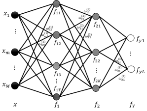
In the context of supervised classification based on MLPs, 𝒴={1,,L}\mathcal{Y}=\{1,\cdots,L\} consists of finite LL labels, and PFY|X(l|xi)P_{F_{Y}|X}(l|x_{i})333For simplicity, PFY|X(l|xi):=P(FY=l|X=xi)P_{F_{Y}|X}(l|x_{i}):=P(F_{Y}=l|X=x_{i}). denotes the prior probability of xix_{i} belonging to class ll based on the hh expressed by MLPs. We define P(FY|X)P^{*}(F_{Y}|X) as the truly prior distribution of the true hh^{*}. Given P(FY|X)P^{*}(F_{Y}|X) and P(Y|FY,X)P(Y|F_{Y},X), P(FY|X,Y)P^{*}(F_{Y}|X,Y) is the truly posterior distribution with the one-hot format, i.e., l𝒴\forall l\in\mathcal{Y}, PFY|X,Y(l|xi,yi)=1P^{*}_{F_{Y}|X,Y}(l|x_{i},y_{i})=1 if l=yil=y_{i}; otherwise PFY|X,Y(l|xi,yi)=0P^{*}_{F_{Y}|X,Y}(l|x_{i},y_{i})=0. We aim to learn an optimal MLP from 𝒮\mathcal{S} such that it approaches P(FY|X,Y)P^{*}(F_{Y}|X,Y) as close as possible. In this paper, we use the MLP={x;f1;f2;fY}\text{MLP}=\{{x;f_{1};f_{2};f_{Y}}\} (Figure 1) for most theoretical derivations unless otherwise specified.

3 Probabilistic Explanations for Multilayer Perceptrons

In this section, we define the probability space (Ω,𝒯,QF)(\Omega,\mathcal{T},Q_{F}) for a fully connected layer, thereby deriving that the entire architecture of the MLP formulates a family of Gibbs distributions Q(FY|X)Q(F_{Y}|X). Moreover, we prove that if \ell is the cross entropy, minimizing ^𝒮(h)\hat{\mathcal{L}}^{\ell}_{\mathcal{S}}(h) can be explained as Bayesian variational inference, and it is equivalent to maximizing Q𝒮(FY|X)=i=1nQFY|X(yi|xi)Q_{\mathcal{S}}(F_{Y}|X)=\prod_{i=1}^{n}Q_{F_{Y}|X}(y_{i}|x_{i}).

Definition 1:

the probability space (Ω,𝒯,QF)(\Omega,\mathcal{T},Q_{F}) for a fully connected layer.

Given a fully connected layer f{f} with TT neurons {ft=σ[gt(xi)]=σ(m=1Mωmtxim+bt)}t=1T\{f_{t}=\sigma[g_{t}({x_{i}})]=\sigma(\sum_{m=1}^{M}\omega_{mt}\cdot x_{im}+b_{t})\}_{t=1}^{T}, where σ()\sigma(\cdot) is an activation function, e.g, ReLU function, xi={xim}m=1M𝒳x_{i}=\{x_{im}\}_{m=1}^{M}\in\mathcal{X} is the input of f{f}, and gt()g_{t}(\cdot) is the ttth linear filter with ωmt\omega_{mt} being the weight and btb_{t} being the bias, let inputting xi{x_{i}} into f{f} be an experiment, we define the probability space (Ω,𝒯,QF)(\Omega,\mathcal{T},Q_{F}) as follows.

First, the sample space Ω\Omega consists of TT possible outcomes {𝝎t}t=1T\{\boldsymbol{\omega}_{t}\}_{t=1}^{T}, where 𝝎t={ωmt}m=1M\boldsymbol{\omega}_{t}=\{\omega_{mt}\}_{m=1}^{M}. In terms of machine learning, a possible outcome 𝝎t\boldsymbol{\omega}_{t} defines a potential feature of xi{x_{i}}. Since scalar values cannot describe the dependence within xi{x_{i}}, we do not take into account btb_{t} for defining Ω\Omega. Second, we define the event space 𝒯\mathcal{T} as the σ\sigma-algebra. For example, if f{f} has T=2T=2 linear filters and Ω={𝝎1,𝝎2}\Omega=\{\boldsymbol{\omega}_{1},\boldsymbol{\omega}_{2}\}, thus 𝒯={,{𝝎1},{𝝎2},{{𝝎1,𝝎2}}{\textstyle\mathcal{T}=\{\emptyset,\{\boldsymbol{\omega}_{1}\},\{\boldsymbol{\omega}_{2}\},\{\{\boldsymbol{\omega}_{1},\boldsymbol{\omega}_{2}\}\}} indicates that none of outcomes, one of outcomes, or both outcomes could happen in the experiment. Third, we prove the probability measure QFQ_{F} as a Gibbs distribution to quantify the probability of possible outcomes {𝝎t}t=1T\{\boldsymbol{\omega}_{t}\}_{t=1}^{T} occurring in xi{x_{i}}.

QF(𝝎t)=1ZF(xi)exp(ft)=1ZF(xi)exp[σ(𝝎t,xi+bt)],Q_{F}(\boldsymbol{\omega}_{t})=\frac{1}{Z_{F}(x_{i})}\text{exp}(f_{t})=\frac{1}{Z_{F}(x_{i})}\text{exp}[\sigma(\langle\boldsymbol{\omega}_{t},{x_{i}}\rangle+b_{t})], (6)

where ,\langle\cdot,\cdot\rangle is the inner product, ZF(xi)=t=1Texp(ft)Z_{F}(x_{i})=\sum_{t=1}^{T}\text{exp}(f_{t}) is the partition function only depending on xix_{i}, and the energy function E𝝎t(xi)E_{\boldsymbol{\omega}_{t}}({x_{i}}) equals the negative activation, i.e., E𝝎t(xi)=ftE_{\boldsymbol{\omega}_{t}}({x_{i}})=-f_{t}. Notably, the higher activation ftf_{t} indicates the lower energy E𝝎t(xi)E_{\boldsymbol{\omega}_{t}}({x_{i}}), thus 𝝎t\boldsymbol{\omega}_{t} has the higher probability of occurring in xi{x_{i}}. The detailed proofs and supportive simulations are presented in Appendix B444We recommend reading the supplementary file connecting the paper and the appendix together.

Based on (Ω,𝒯,QF)(\Omega,\mathcal{T},Q_{F}) for the fully connected layer f{f}, we can explicitly define the corresponding random variable F:ΩEF:\Omega\rightarrow E. Specifically, since Ω={𝝎t}t=1T\Omega=\{\boldsymbol{\omega}_{t}\}_{t=1}^{T} includes finite TT possible outcomes, EE should be a discrete measurable space and FF is a discrete random variable. For example, Q(F=t)Q(F=t) indicates the probability of the ttth outcome 𝝎t\boldsymbol{\omega}_{t} occurring in xi{x_{i}}. Furthermore, the probability space of a fully connected layer enables us to derive probabilistic explanations for MLPs.

Theorem 2:

the MLP={x;f1;f2;fY}\text{MLP}=\{{x;f_{1};f_{2};f_{Y}}\} corresponds to a family of Gibbs distributions

QFY|X(l|xi)=1ZMLP(xi)exp[Eyl(xi)]=1ZMLP(xi)exp[fyl(f2(f1(xi)))],Q_{F_{Y}|X}(l|x_{i})=\frac{1}{Z_{\text{MLP}}(x_{i})}\text{exp}[-E_{yl}(x_{i})]=\frac{1}{Z_{\text{MLP}}(x_{i})}\text{exp}[{f_{yl}(f_{2}(f_{1}({x_{i}})))}], (7)

where Eyl(xi)=fyl(f2(f1(xi)))E_{yl}(x_{i})=-{f_{yl}(f_{2}(f_{1}(x_{i})))} is the energy function of l𝒴l\in\mathcal{Y} given xix_{i}, and the partition function ZMLP(xi)=l=1Lk=1Kt=1TQ(FY,F2,F1|X=xi)Z_{\text{MLP}}(x_{i})=\sum_{l=1}^{L}\sum_{k=1}^{K}\sum_{t=1}^{T}Q(F_{Y},F_{2},F_{1}|X=x_{i}).

Proof: Definition 1 implies ωmt\omega_{mt} defining Ω\Omega, thus Ω\Omega would be fixed if not considering training. Therefore, Fi+1{F_{i+1}} is entirely determined by Fi{F_{i}} in the MLP, where FiF_{i} denotes the random variable of fif_{i}, and the MLP forms a Markov chain XF1F2FY{X}\boldsymbol{\leftrightarrow}{F_{1}}\boldsymbol{\leftrightarrow}{F_{2}}{\leftrightarrow}{F_{Y}}. As a result, given a sample x=xix=x_{i}, the conditional distribution Q(FY|X)Q(F_{Y}|X) corresponding to the MLP can be derived as

QFY|X(l|xi)=k=1Kt=1TQFY,F2,F1|X(l,k,t|xi)=1ZMLP(xi)exp[fyl(f2(f1(xi)))].Q_{F_{Y}|X}(l|x_{i})=\sum_{k=1}^{K}\sum_{t=1}^{T}Q_{F_{Y},F_{2},F_{1}|X}(l,k,t|x_{i})=\frac{1}{Z_{\text{MLP}}(x_{i})}\text{exp}[{f_{yl}(f_{2}(f_{1}({x_{i}})))}]. (8)

The derivation is presented in Appendix C. The energy function Eyl(xi)=fyl(f2(f1(xi)))E_{yl}(x_{i})=-{f_{yl}(f_{2}(f_{1}(x_{i})))} implies that QFY|X(l|xi)Q_{F_{Y}|X}(l|x_{i}) is entirely determined by the architecture of the MLP. In other words, the MLP formulates a family of Gibbs distributions Q(FY|X)Q(F_{Y}|{X}).

Corollary 1:

Given the samples 𝒮\mathcal{S} and the MLP={x;f1;f2;fY}\text{MLP}=\{{x;f_{1};f_{2};f_{Y}}\}, if \ell is the cross entropy, then minimizing ^𝒮(h)\hat{\mathcal{L}}^{\ell}_{\mathcal{S}}(h) is equivalent to maximizing Q𝒮(FY|X)Q_{\mathcal{S}}(F_{Y}|X).

minh^𝒮(h)maxQ(FY|X)1nlogQ𝒮(FY|X),\underset{h\in\mathcal{H}}{\text{min}}\hat{\mathcal{L}}^{\ell}_{\mathcal{S}}(h)\Rightarrow\underset{Q(F_{Y}|X)}{\text{max}}\frac{1}{n}\text{log}Q_{\mathcal{S}}(F_{Y}|X), (9)

where Q𝒮(FY|X)=i=1nQFY|X(yi|xi)Q_{\mathcal{S}}(F_{Y}|X)=\prod_{i=1}^{n}Q_{F_{Y}|X}(y_{i}|x_{i}).

Proof: since the cross entropy H[P(FY|X,Y),Q(FY|X)]=𝑬P(FY|X,Y)[logQ(FY|X)]H[P^{*}(F_{Y}|X,Y),Q(F_{Y}|X)]=\underset{P^{*}(F_{Y}|X,Y)}{-\boldsymbol{E}}[\text{log}Q(F_{Y}|X)], we have

^𝒮(h)=1ni=1nH[P(FY|X,Y),Q(FY|X)]=1ni=1nl=1LPFY|X,Y(l|xi,yi)logQFY|X(l|xi).\hat{\mathcal{L}}^{\ell}_{\mathcal{S}}(h)=-\frac{1}{n}\sum_{i=1}^{n}H[P^{*}(F_{Y}|X,Y),Q(F_{Y}|X)]=-\frac{1}{n}\sum_{i=1}^{n}\sum_{l=1}^{L}P^{*}_{F_{Y}|X,Y}(l|x_{i},y_{i})\text{log}Q_{F_{Y}|X}(l|x_{i}). (10)

Since P(FY|X,Y)P^{*}(F_{Y}|X,Y) is one-hot, namely that if l=yil=y_{i}, then PFY|X,Y(l|xi,yi)=1P^{*}_{F_{Y}|X,Y}(l|x_{i},y_{i})=1, otherwise PFY|X,Y(l|xi,yi)=0P^{*}_{F_{Y}|X,Y}(l|x_{i},y_{i})=0, we can simplify Equation (10) as

^𝒮(h)=1ni=1nlogQFY|X(yi|xi)=1nlogQ𝒮(FY|X).\hat{\mathcal{L}}^{\ell}_{\mathcal{S}}(h)=-\frac{1}{n}\sum_{i=1}^{n}\text{log}Q_{F_{Y}|X}(y_{i}|x_{i})=-\frac{1}{n}\text{log}Q_{\mathcal{S}}(F_{Y}|X). (11)

Therefore, minimizing ^𝒮(h)\hat{\mathcal{L}}^{\ell}_{\mathcal{S}}(h) is equivalent to maximizing the likelihood Q𝒮(FY|X)Q_{\mathcal{S}}(F_{Y}|X). In addition, based on Theorem 2 (Equation 7), we can extend ^𝒮(h)\hat{\mathcal{L}}^{\ell}_{\mathcal{S}}(h) as

n^𝒮(h)=i=1nlogQFY|X(yi|xi)=i=1n[Eyyi(xi)+logZMLP(xi)].n\hat{\mathcal{L}}^{\ell}_{\mathcal{S}}(h)=-\sum_{i=1}^{n}\text{log}Q_{F_{Y}|X}(y_{i}|x_{i})=\sum_{i=1}^{n}[E_{yy_{i}}(x_{i})+\text{log}Z_{\text{MLP}}(x_{i})]. (12)

Recall that ZMLP(xi)=l=1Lk=1Kt=1TQ(FY,F2,F1|X=xi)Z_{\text{MLP}}(x_{i})=\sum_{l=1}^{L}\sum_{k=1}^{K}\sum_{t=1}^{T}Q(F_{Y},F_{2},F_{1}|X=x_{i}) sums up all the cases of FYF_{Y}, thus logZMLP(xi)\text{log}Z_{\text{MLP}}(x_{i}) can be viewed as a constant with respect to Q(FY|X)Q(F_{Y}|X).

Theorem 3:

given the samples 𝒮\mathcal{S} and the MLP={x;f1;f2;fY}\text{MLP}=\{{x;f_{1};f_{2};f_{Y}}\}, if \ell is the cross entropy, then minimizing ^𝒮(h)\hat{\mathcal{L}}^{\ell}_{\mathcal{S}}(h) can be explained as Bayesian variational inference.

minh^𝒮(h)minQ(FY|X)KL[Q𝒮x(FY|X)||P𝒮(FY|X,Y)],\underset{h\in\mathcal{H}}{\text{min}}\hat{\mathcal{L}}^{\ell}_{\mathcal{S}}(h)\Rightarrow\underset{Q(F_{Y}|X)}{\text{min}}\text{KL}[Q_{\mathcal{S}_{x}}(F_{Y}|X)||P^{*}_{\mathcal{S}}(F_{Y}|X,Y)], (13)

where Q𝒮x(FY|X)=i=1nQ(FY|X=xi)Q_{\mathcal{S}_{x}}(F_{Y}|X)=\prod_{i=1}^{n}Q(F_{Y}|X=x_{i}) and P𝒮(FY|X,Y)=i=1nP(FY|X=xi,Y=yi)P^{*}_{\mathcal{S}}(F_{Y}|X,Y)=\prod_{i=1}^{n}P^{*}(F_{Y}|X=x_{i},Y=y_{i}).

Proof: based on the property H(P,Q)=H(P)+KL[P||Q]H(P,Q)=H(P)+\text{KL}[P||Q], we can derive ^𝒮(h)\hat{\mathcal{L}}^{\ell}_{\mathcal{S}}(h) as

^𝒮(h)=1ni=1nH[P(FY|X=xi,Y=yi)]+KL[P(FY|X=xi,Y=yi)||Q(FY|X=xi)].\hat{\mathcal{L}}^{\ell}_{\mathcal{S}}(h)=\frac{1}{n}\sum_{i=1}^{n}H[{P^{*}(F_{Y}|X=x_{i},Y=y_{i})}]+\text{KL}[{P^{*}(F_{Y}|X=x_{i},Y=y_{i})||Q(F_{Y}|X=x_{i})}]. (14)

Since PFY|X,Y(l|xi,yi)P^{*}_{F_{Y}|X,Y}(l|x_{i},y_{i}) is one-hot, namely that if l=yil=y_{i}, PFY|X,Y(l|xi,yi)=1P^{*}_{F_{Y}|X,Y}(l|x_{i},y_{i})=1, otherwise PFY|X,Y(l|xi,yi)=0P^{*}_{F_{Y}|X,Y}(l|x_{i},y_{i})=0, H[P(FY|X=xi,Y=yi)]=0H[P^{*}(F_{Y}|X=x_{i},Y=y_{i})]=0, thus we can simplify ^𝒮(h)\hat{\mathcal{L}}^{\ell}_{\mathcal{S}}(h) as

^𝒮(h)=1ni=1nKL[P(FY|X=xi,Y=yi)||Q(FY|X=xi)].\hat{\mathcal{L}}^{\ell}_{\mathcal{S}}(h)=\frac{1}{n}\sum_{i=1}^{n}\text{KL}[P^{*}(F_{Y}|X=x_{i},Y=y_{i})||Q(F_{Y}|X=x_{i})]. (15)

To keep consistent with the definition of variational inference, we reformulate ^𝒮(h)\hat{\mathcal{L}}^{\ell}_{\mathcal{S}}(h) as

^𝒮(h)=1ni=1n{KL[Q(FY|X=xi)||P(FY|X=xi,Y=yi)]+d}.\hat{\mathcal{L}}^{\ell}_{\mathcal{S}}(h)=\frac{1}{n}\sum_{i=1}^{n}\{\text{KL}[Q(F_{Y}|X=x_{i})||P^{*}(F_{Y}|X=x_{i},Y=y_{i})]+d\}. (16)

where d=KL[P(FY|X,Y)||Q(FY|X)]KL[Q(FY|X)||P(FY|X,Y)]d=\text{KL}[P^{*}(F_{Y}|X,Y)||Q(F_{Y}|X)]-\text{KL}[Q(F_{Y}|X)||P^{*}(F_{Y}|X,Y)].

Though KL-divergence is asymmetric, i.e., KL[P||Q]KL[Q||P]\text{KL}[P||Q]\neq\text{KL}[Q||P], we show that dd converges to zero during minimizing ^𝒮(h)\hat{\mathcal{L}}^{\ell}_{\mathcal{S}}(h), because P(FY|X,Y)P^{*}(F_{Y}|X,Y) is fixed and Q(FY|X)Q(F_{Y}|X) is the only variable. The proof for d0d\rightarrow 0 is presented in Appendix D. Moreover, since 𝒮\mathcal{S} consists of i.i.d. samples and KL-divergence is additive for independent distributions, we can finally derive

minhn^𝒮(h)=minQ(FY|X)KL[Q𝒮x(FY|X)||P𝒮(FY|X,Y)].\underset{h\in\mathcal{H}}{\text{min}}n\hat{\mathcal{L}}^{\ell}_{\mathcal{S}}(h)=\underset{Q(F_{Y}|X)}{\text{min}}\text{KL}[Q_{\mathcal{S}_{x}}(F_{Y}|X)||P^{*}_{\mathcal{S}}(F_{Y}|X,Y)]. (17)

As a result, minimizing n^𝒮(h)n\hat{\mathcal{L}}^{\ell}_{\mathcal{S}}(h) with the cross entropy loss is equivalent to Bayesian variational inference. In summary, Theorem 3 provides a novel probabilistic explanation for MLPs from the perspective of Bayesian variational inference. Specifically, the MLP formulates a family of Gibbs distribution Q(FY|X)Q(F_{Y}|X), and minimizing ^𝒮(h)\hat{\mathcal{L}}^{\ell}_{\mathcal{S}}(h) aims to search an optimal distribution Q(FY|X)Q(F_{Y}|X), which is closest to the truly posterior distribution P(FY|X,Y)P^{*}(F_{Y}|X,Y) given 𝒮\mathcal{S}.

4 PAC-Bayesian Bounds for Multilayer Perceptrons

In this section, we prove that MLPs with the cross entropy loss inherently guarantee PAC-Bayesian generalization bounds based on the ELBO derived from Bayesian variational inference. Moreover, we derive a novel PAC-Bayesian generalization bound for MLPs.

Theorem 4:

given the samples 𝒮\mathcal{S} and the MLP={x;f1;f2;fY}\text{MLP}=\{{x;f_{1};f_{2};f_{Y}}\}, if ^𝒮(h)\hat{\mathcal{L}}^{\ell}_{\mathcal{S}}(h) is the cross entropy, then minimizing ^𝒮(h)\hat{\mathcal{L}}^{\ell}_{\mathcal{S}}(h) inherently guarantees PAC-Bayesian generalization bounds for the MLP.

minh^𝒮(h)minQ(F|X)KL[Q𝒮x(FY|X)||P𝒮(FY|X,Y)]Bayesian variational inferencemin 𝜌n𝑬hρ^𝒮(h)+KL[ρ||π]PAC-Bayesian optimization.\underset{h\in\mathcal{H}}{\text{min}}\hat{\mathcal{L}}^{\ell}_{\mathcal{S}}(h)\Rightarrow\underbrace{\underset{Q(F|X)}{\text{min}}\text{KL}[Q_{\mathcal{S}_{x}}(F_{Y}|X)||P^{*}_{\mathcal{S}}(F_{Y}|X,Y)]}_{\text{Bayesian variational inference}}\Rightarrow\underbrace{\underset{\rho}{\text{min }}n\underset{h\sim\rho}{\boldsymbol{E}}\hat{\mathcal{L}}^{\ell}_{\mathcal{S}}(h)+\text{KL}[\rho||\pi]}_{\text{PAC-Bayesian optimization}}. (18)

Proof: we only need prove Bayesian variational inference inducing PAC-Bayesian generalization bounds based on Theorem 3. Given the Bayesian variational inference (Equation 17), we have

KL[Q𝒮x(FY|X)||P𝒮(FY|X,Y)]=𝑬Q(FY|X)logQ𝒮x(FY|X)𝑬Q(FY|X)logP𝒮(FY|X,Y)=𝑬Q(FY|X)logQ𝒮x(FY|X)𝑬Q(FY|X)[logP𝒮(FY,Y|X)logP𝒮(Y|X)].\begin{split}\text{KL}[{\scriptstyle Q_{\mathcal{S}_{x}}(F_{Y}|X)}||{\scriptstyle P^{*}_{\mathcal{S}}(F_{Y}|X,Y)}]=&\underset{Q(F_{Y}|X)}{\boldsymbol{E}}\text{log}{\scriptstyle Q_{\mathcal{S}_{x}}(F_{Y}|X)}-\underset{Q(F_{Y}|X)}{\boldsymbol{E}}\text{log}{\scriptstyle P^{*}_{\mathcal{S}}(F_{Y}|X,Y)}\\ =&\underset{Q(F_{Y}|X)}{\boldsymbol{E}}\text{log}{\scriptstyle Q_{\mathcal{S}_{x}}(F_{Y}|X)}-\underset{Q(F_{Y}|X)}{\boldsymbol{E}}[\text{log}{\scriptstyle P^{*}_{\mathcal{S}}(F_{Y},Y|X)}-\text{log}{\scriptstyle P_{\mathcal{S}}(Y|X)}].\end{split} (19)

Since logP𝒮(Y|X)\text{log}P_{\mathcal{S}}(Y|X) is constant with respect to Q(FY|X)Q(F_{Y}|X), we can derive the ELBO as

logP𝒮(Y|X)=𝑬Q(FY|X)logP𝒮(Y|FY,X)KL[Q𝒮x(FY|X)||P𝒮x(FY|X)]ELBO+KL[Q𝒮x(FY|X)||P𝒮(FY|X,Y)],\text{log}P_{\mathcal{S}}(Y|X)=\underbrace{\underset{Q(F_{Y}|X)}{\boldsymbol{E}}\text{log}{\scriptstyle P_{\mathcal{S}}(Y|F_{Y},X)}-\text{KL}[{\scriptstyle Q_{\mathcal{S}_{x}}(F_{Y}|X)}||{\scriptstyle P^{*}_{\mathcal{S}_{x}}(F_{Y}|X)}]}_{\text{ELBO}}+\text{KL}[{\scriptstyle Q_{\mathcal{S}_{x}}(F_{Y}|X)}||{\scriptstyle P^{*}_{\mathcal{S}}(F_{Y}|X,Y)}], (20)

where P𝒮(Y|X)=i=1nP(Y=yi|X=xi)P_{\mathcal{S}}(Y|X)=\prod_{i=1}^{n}P(Y=y_{i}|X=x_{i}), P𝒮(Y|FY,X)=i=1nP(Y=yi|FY,X=xi)P_{\mathcal{S}}(Y|F_{Y},X)=\prod_{i=1}^{n}P(Y=y_{i}|F_{Y},X=x_{i}), Q𝒮x(FY|X)=i=1nQ(FY|X=xi)Q_{\mathcal{S}_{x}}(F_{Y}|X)=\prod_{i=1}^{n}Q(F_{Y}|X=x_{i}), and P𝒮x(FY|X)=i=1nP(FY|X=xi)P^{*}_{\mathcal{S}_{x}}(F_{Y}|X)=\prod_{i=1}^{n}P^{*}(F_{Y}|X=x_{i}). The detailed derivation of the ELBO is presented in Appendix E.

Since P(FY|X)P^{*}(F_{Y}|X) is the truly prior distribution of the true hypothesis hh^{*}, we have π:=P𝒮x(FY|X)\pi:=P^{*}_{\mathcal{S}_{x}}(F_{Y}|X). Since Q(FY|X)Q(F_{Y}|X) infers the truly posterior distribution P(FY|X,Y)P^{*}(F_{Y}|X,Y) of hh, we have ρ:=Q𝒮x(FY|X)\rho:=Q_{\mathcal{S}_{x}}(F_{Y}|X). Corollary 1 induces n^𝒮(h)=logP𝒮(Y|FY,X)n\hat{\mathcal{L}}^{\ell}_{\mathcal{S}}(h)=-\text{log}P_{\mathcal{S}}(Y|F_{Y},X) because we can express P(Y=yi|FY,X=xi)P(Y=y_{i}|F_{Y},X=x_{i}) as Q(FY=yi|X=xi)Q(F_{Y}=y_{i}|X=x_{i}). As a result, we derive

ELBO=(n𝑬Q(FY|X)^𝒮(h)+KL[Q𝒮x(FY|X)||P𝒮x(FY|X)]).\text{ELBO}=-(n\underset{Q(F_{Y}|X)}{\boldsymbol{E}}{\hat{\mathcal{L}}^{\ell}_{\mathcal{S}}(h)}+\text{KL}[{Q_{\mathcal{S}_{x}}(F_{Y}|X)}||{P^{*}_{\mathcal{S}_{x}}(F_{Y}|X)}]). (21)

It implies that maximizing ELBO is equivalent to minimizing PAC-Bayesian generalization bounds, thus minimizing ^𝒮(h)\hat{\mathcal{L}}^{\ell}_{\mathcal{S}}(h) inherently guarantees PAC-Bayesian generalization bounds for the MLP.

Theorem 4 theoretically explains why MLPs can achieve great generalization performance without explicit regularization. More specifically, the ELBO indicates that minimizing ^𝒮(h)\hat{\mathcal{L}}^{\ell}_{\mathcal{S}}(h) makes MLPs not only to learn the likelihood P𝒮(Y|FY,X)P_{\mathcal{S}}(Y|F_{Y},X) but also to learn the prior knowledge via minimizing KL[Q𝒮x(FY|X)||P𝒮x(FY|X)]\text{KL}[{\scriptstyle Q_{\mathcal{S}_{x}}(F_{Y}|X)}||{\scriptstyle P^{*}_{\mathcal{S}_{x}}(F_{Y}|X)}]. In other words, minimizing ^𝒮(h)\hat{\mathcal{L}}^{\ell}_{\mathcal{S}}(h) inherently guarantees PAC-Bayesian generalization bounds for MLPs, even though they do not incorporate explicit regularization.

Corollary 2:

PAC-Bayesian generalization bounds for the MLP.

Given a distribution 𝒟\mathcal{D} over 𝒳×𝒴\mathcal{X}\times\mathcal{Y}, the samples 𝒮\mathcal{S}, a probabilistic hypothesis set \mathcal{H} derived from the MLP={x;f1;f2;fY}\text{MLP}=\{{x;f_{1};f_{2};f_{Y}}\}, the cross entropy loss :×𝒳×𝒴+\ell:\mathcal{F}\times\mathcal{X}\times\mathcal{Y}\rightarrow\mathbb{R}^{+} 555The previous works prove PAC-Bayesian bounds being valid for unbounded loss functions [10, 2]., a real number b>0b>0, and a real number δ(0,1]\delta\in(0,1], with probability at least 1δ1-\delta over the samples 𝒮𝒟n\mathcal{S}\sim\mathcal{D}^{n}, we have

Q(FY|X) on :𝑬hQ(FY|X)𝒟(h)b1eb{1δP𝒮(Y|X)nexp(1ni=1n[Eyyi(xi)+logZMLP(xi)])}.\forall Q(F_{Y}|X)\text{ on }\mathcal{H}:\underset{{h\sim Q(F_{Y}|X)}}{\boldsymbol{E}}\mathcal{L}^{\ell}_{\mathcal{D}}(h)\leq\frac{b}{1-e^{-b}}\{1-\frac{\sqrt[n]{\delta\cdot P_{\mathcal{S}}(Y|X)}}{\text{exp}(\frac{1}{n}\sum_{i=1}^{n}[E_{yy_{i}}(x_{i})+\text{log}Z_{\text{MLP}}(x_{i})])}\}. (22)

where P𝒮(Y|X)=i=1nPY|X(yi|xi)P_{\mathcal{S}}(Y|X)=\prod_{i=1}^{n}P_{Y|X}(y_{i}|x_{i}), Eyyi(xi)=fyyi(f2(f1(xi)))E_{yy_{i}}(x_{i})=-f_{yy_{i}}(f_{2}(f_{1}(x_{i}))) is the energy of yiy_{i} given xix_{i}, and ZMLP(xi)=l=1Lk=1Kt=1TP(FY,F2,F1|X=xi)Z_{\text{MLP}}(x_{i})=\sum_{l=1}^{L}\sum_{k=1}^{K}\sum_{t=1}^{T}P(F_{Y},F_{2},F_{1}|X=x_{i}) is the partition function.

Proof: the result is derived by two steps: (i) substituting n𝑬hρ^𝒮(h)+KL[ρ||π]n\underset{h\sim\rho}{\boldsymbol{E}}\hat{\mathcal{L}}^{\ell}_{\mathcal{S}}(h)+\text{KL}[\rho||\pi] in Equation 3 for the ELBO=logP𝒮(Y|X)KL[Q𝒮x(FY|X)||P𝒮(FY|X,Y)]\text{ELBO}=\text{log}P_{\mathcal{S}}(Y|X)-\text{KL}[{\scriptstyle Q_{\mathcal{S}_{x}}(F_{Y}|X)}||{\scriptstyle P^{*}_{\mathcal{S}}(F_{Y}|X,Y)}] in Equation 20; and (ii) substituting KL[Q𝒮x(FY|X)||P𝒮(FY|X,Y)]\text{KL}[{\scriptstyle Q_{\mathcal{S}_{x}}(F_{Y}|X)}||{\scriptstyle P^{*}_{\mathcal{S}}(F_{Y}|X,Y)}] for i=1n[Eyyi(xi)+logZMLP(xi)]\sum_{i=1}^{n}[E_{yy_{i}}(x_{i})+\text{log}Z_{\text{MLP}}(x_{i})] based on Equation 17 and 12.

Corollary 1 implies that when minimizing ^𝒮(h)\hat{\mathcal{L}}^{\ell}_{\mathcal{S}}(h) to zero, 1ni=1n[Eyyi(xi)+logZMLP(xi)]0\frac{1}{n}\sum_{i=1}^{n}[E_{yy_{i}}(x_{i})+\text{log}Z_{\text{MLP}}(x_{i})]\rightarrow 0 and the proposed PAC-Bayesian generalization bound would be entirely determined by the marginal likelihood P𝒮(Y|X)P_{\mathcal{S}}(Y|X), which is consistent with the theoretical connection between PAC-Bayesian theory and Bayesian inference proposed by Germain et al. [10].

Based on Corollary 2, we derive an applicable bound for examining the generalization of MLPs. Though P(Y|X)P(Y|X) is unknown, the i.i.d. assumption for 𝒮\mathcal{S} induces P𝒮(Y|X)n=P(Y|X)\sqrt[n]{P_{\mathcal{S}}(Y|X)}=P(Y|X) being a constant as long as the number of different labels are equivalent. As a result, we have

the PAC-Bayesian generalization boundexp(1ni=1n[Eyyi(xi)+logZMLP(xi)]).\text{the PAC-Bayesian generalization bound}\propto\text{exp}(\frac{1}{n}\sum_{i=1}^{n}[E_{yy_{i}}(x_{i})+\text{log}Z_{\text{MLP}}(x_{i})]). (23)

Recall that ZMLP(xi)=l=1Lk=1Kt=1TQ(FY,F2,F1|X=xi)Z_{\text{MLP}}(x_{i})=\sum_{l=1}^{L}\sum_{k=1}^{K}\sum_{t=1}^{T}Q(F_{Y},F_{2},F_{1}|X=x_{i}) sums up all the cases of FYF_{Y}, i.e., ZMLP(xi)Z_{\text{MLP}}(x_{i}) is a constant with respect to Q(FY|X)Q(F_{Y}|X). In addition, we show that the functionality of ZMLP(xi)Z_{\text{MLP}}(x_{i}) is only to guarantee the validity of Q(FY|X)Q(F_{Y}|X) (Appendix F). Therefore, i=1nlogZMLP(xi)\sum_{i=1}^{n}\text{log}Z_{\text{MLP}}(x_{i}) can be viewed as a constant for deriving PAC-Bayesian generalization bounds for MLPs, thus the bound can be further relaxed as

the PAC-Bayesian generalization bound1ni=1nEyyi(xi).\text{the PAC-Bayesian generalization bound}\propto\frac{1}{n}\sum_{i=1}^{n}E_{yy_{i}}(x_{i}). (24)

We use the above formula to approximate the generalization bound for subsequent experiments.

5 Experimental Results

In this section, we demonstrate the proposed PAC-Bayesian generalization bound on MLPs in four different cases: (i) different training algorithms, (ii) different architectures of MLPs, (iii) different sample sizes, and (iv) different labels, namely real labels and random labels.

All the experimental results are derived based on the MLP={x;f1;f2;fY}\text{MLP}=\{{x;f_{1};f_{2};f_{Y}}\} classifying the MNIST dataset [17]. Since the dimension of a single MNIST image is 28×2828\times 28, xx has M=784M=784 input nodes. Since the MNIST dataset consists of 1010 different labels, fY{f_{Y}} has L=10L=10 output nodes. All the activation functions are ReLU σ(z):=max(0,z)\sigma(z):=\text{max}(0,z). Because of space limitation, we present more experimental results based on MLPs on other benchmark datasets in Appendix G.

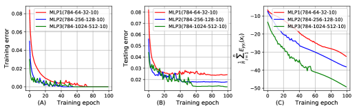
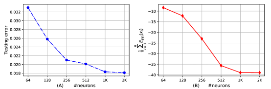
The bound can reflect the generalization of MLPs with different number of neurons [30].

We design three MLPs (abbr. MLP1, MLP2, MLP3). They have the same architecture except the number of neurons in hidden layers, which are summarized in Figure 2. We use the same SGD optimization algorithm to train the three MLPs and all the three MLPs achieve zero training error. We visualize the training error, the testing error, and the bound in Figure 2, which shows that the bound has the same architecture dependence as the testing error. In other words, the MLP with the more number of neurons has the lower testing error and bound.

Refer to caption
Figure 2: (A), (B), and (C) show the training error, the testing error, and the bound over 100 training epochs, respectively. In the legend, (M-T-K-L) denotes the number of nodes/neurons in each layer, e.g., MLP1 has T=64T=64 neurons in f1f_{1} and K=32K=32 neurons in f2f_{2}.

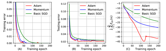
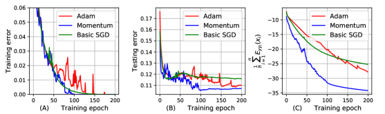
The bound can reflect the effect of SGD optimization on the generalization of MLPs [30].

We use three different training algorithms (the basic SGD [35], Momentum [34], and Adam [16]) to train MLP2 200 epochs, and visualize the training error, the testing error, and the generalization bound in Figure 3. We can observe that the bounds of MLP2 with different training algorithms is consistent with the corresponding testing errors of MLP2. For example, MLP2 with Adam training algorithm achieves the smallest testing error, thus the bound of MLP2 with Adam is also smaller than Momentum and the basic SGD.

Refer to caption
Figure 3: (A), (B), and (C) show the training error, the testing error, and the proposed PAC-Bayesian generalization bound over 200 training epochs, respectively.
Refer to caption
Figure 4: (A) and (B) show the testing error and the bound given different training sample sizes.

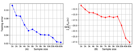
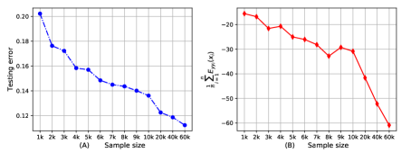
The bound can reflect the same sample size dependence as the testing error [29].

We create 13 different subsets of the MNIST dataset with different number of training samples, and train MLP2 to classify these samples until the training error becomes zero. Figure 4 shows the testing error and the bound with different sample sizes. The bound shows a general decreasing trend as the training sample size increases, which is consistent with the variation of the testing error.

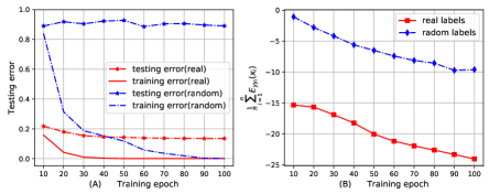
The bound can reflect the generalization performance of MLPs given random labels.

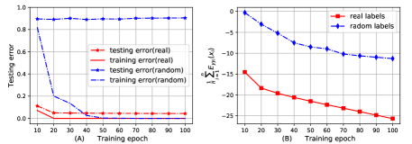
Zhang et al.[38] show that DNNs achieve low testing error when they are trained by random labels. We train MLP3 100 epochs to classify 10,000 samples of the MNIST dataset with random labels, and visualize the training error, the testing error and the bound in Figure 5.

We observe that the bound of MLP3 trained by random labels is higher than real labels, which is consistent with the testing error based on random labels is higher than real labels. In particular, we can theoretically explain why MLP3 trained by random labels has the higher testing error. Random labels imply that YY not depends on FYF_{Y} and XX, i.e., P𝒮(Y|X)=P𝒮(Y|FY,X)=P𝒮(Y)P_{\mathcal{S}}(Y|X)=P_{\mathcal{S}}(Y|F_{Y},X)=P_{\mathcal{S}}(Y), thus the ELBO (Equation 20) can be reformulated as

logP𝒮(Y)=logP𝒮(Y)KL[Q𝒮x(FY|X)||P𝒮x(FY|X)]ELBO+KL[Q𝒮x(FY|X)||P𝒮(FY|X,Y)].\text{log}P_{\mathcal{S}}(Y)=\underbrace{\text{log}{P_{\mathcal{S}}(Y)}-\text{KL}[{\scriptstyle Q_{\mathcal{S}_{x}}(F_{Y}|X)}||{\scriptstyle P^{*}_{\mathcal{S}_{x}}(F_{Y}|X)}]}_{\text{ELBO}}+\text{KL}[{\scriptstyle Q_{\mathcal{S}_{x}}(F_{Y}|X)}||{\scriptstyle P^{*}_{\mathcal{S}}(F_{Y}|X,Y)}]. (25)

As a result, minimizing KL[Q𝒮x(FY|X)||P𝒮(FY|X,Y)]\text{KL}[{\scriptstyle Q_{\mathcal{S}_{x}}(F_{Y}|X)}||{\scriptstyle P^{*}_{\mathcal{S}}(F_{Y}|X,Y)}] equals minimizing KL[Q𝒮x(FY|X)||P𝒮x(FY|X)]\text{KL}[{\scriptstyle Q_{\mathcal{S}_{x}}(F_{Y}|X)}||{\scriptstyle P^{*}_{\mathcal{S}_{x}}(F_{Y}|X)}], which is only one part of the PAC-Bayesian optimization (Equation 4). Therefore, MLPs with random labels cannot guarantee PAC-Bayesian generalization bounds.

Refer to caption
Figure 5: (A) and (B) show the training/testing error and the bound given real and random labels.

6 Conclusions

In this work, we prove that MLPs with the cross entropy loss inherently guarantee PAC-Bayesian generalization bounds, and minimizing PAC-Bayesian generalization bounds for MLPs is equivalent to maximizing the ELBO. In addition, we derive a novel PAC-Bayesian generalization bound correctly explaining the generalization performance of MLPs. Extending the proposed PAC-Bayesian generalization bounds to general DNNs is promising for future work.

References

  • [1] Zeyuan Allen-Zhu, Yuanzhi Li, and Yingyu Liang. Learning and generalization in overparameterized neural networks, going beyond two layers. In Advances in neural information processing systems, pages 6155–6166, 2019.
  • [2] Pierre Alquier, James Ridgway, and Nicolas Chopin. On the properties of variational approximations of gibbs posteriors. The Journal of Machine Learning Research, 17(1):8374–8414, 2016.
  • [3] Amiran Ambroladze, Emilio Parrado-Hernández, and John S Shawe-taylor. Tighter pac-bayes bounds. In Advances in neural information processing systems, pages 9–16, 2007.
  • [4] Roberto Battiti. First and second order methods for learning: Between steepest descent and newton’s method. Neural Computation, 4:141–166, 1992.
  • [5] David Blei, Alp Kucukelbir, and Jon MaAuliffe. Variational inference: A review for statisticians. Journal of Machine Learning Research, 112:859–877, 2017.
  • [6] Olivier Catoni. Pac-bayesian supervised classification: the thermodynamics of statistical learning. arXiv preprint arXiv:0712.0248, 2007.
  • [7] Pratik Chaudhari and Stefano Soatto. Stochastic gradient descent performs variational inference, converges to limit cycles for deep networks. In 2018 Information Theory and Applications Workshop (ITA), pages 1–10. IEEE, 2018.
  • [8] Gintare Karolina Dziugaite and Daniel M Roy. Computing nonvacuous generalization bounds for deep (stochastic) neural networks with many more parameters than training data. arXiv preprint arXiv:1703.11008, 2017.
  • [9] S. Geman and D. Geman. Stochastic relaxation, gibbs distributions, and the bayesian restoration of images. IEEE Transactions. on Pattern Analysis and Machine Intelligence, pages 721–741, June 1984.
  • [10] Pascal Germain, Francis Bach, Alexandre Lacoste, and Simon Lacoste-Julien. Pac-bayesian theory meets bayesian inference. In Advances in Neural Information Processing Systems, pages 1884–1892, 2016.
  • [11] Pascal Germain, Alexandre Lacasse, François Laviolette, and Mario Marchand. Pac-bayesian learning of linear classifiers. In Proceedings of the 26th Annual International Conference on Machine Learning, pages 353–360, 2009.
  • [12] Geoffrey E Hinton. Training products of experts by minimizing contrastive divergence. Neural Computation, 14:1771–1800, 2002.
  • [13] Elad Hoffer, Itay Hubara, and Daniel Soudry. Train longer, generalize better: closing the generalization gap in large batch training of neural networks. In Advances in Neural Information Processing Systems, pages 1731–1741, 2017.
  • [14] Matthew D. Hoffman, David M. Blei, Chong Wang, and John Paisley. Stochastic variational inference. Journal of Machine Learning Research, 14:1303–1347, 2013.
  • [15] Kenji Kawaguchi, Leslie Pack Kaelbling, and Yoshua Bengio. Generalization in deep learning. arXiv preprint arXiv:1710.05468, 2017.
  • [16] Diederik P Kingma and Jimmy Ba. Adam: A method for stochastic optimization. arXiv preprint arXiv:1412.6980, 2014.
  • [17] Y. LeCun, L. Bottou, and P. Haffner. Gradient-based learning applied to document recognition. Proceedings of the IEEE, 11:2278–2324, 1998.
  • [18] Yann LeCun, Sumit Chopra, Raia Hadsell, Marc’Aurelio Ranzato, and Fu Jie Huang. A tutorial on energy-based learning. MIT Press, 2006.
  • [19] Gaël Letarte, Pascal Germain, Benjamin Guedj, and François Laviolette. Dichotomize and generalize: Pac-bayesian binary activated deep neural networks. In Advances in Neural Information Processing Systems, pages 6869–6879, 2019.
  • [20] Guy Lever, François Laviolette, and John Shawe-Taylor. Tighter pac-bayes bounds through distribution-dependent priors. Theor. Comput. Sci., 473(Feb):4–28, 2013.
  • [21] Yuanzhi Li and Yingyu Liang. Learning overparameterized neural networks via stochastic gradient descent on structured data. In Advances in Neural Information Processing Systems, pages 8157–8166, 2018.
  • [22] Henry W Lin, Max Tegmark, and David Rolnick. Why does deep and cheap learning work so well? Journal of Statistical Physics, 168(6):1223–1247, 2017.
  • [23] Ben London. A pac-bayesian analysis of randomized learning with application to stochastic gradient descent. In Advances in Neural Information Processing Systems, pages 2931–2940, 2017.
  • [24] Stephan Mandt, Matthew D Hoffman, and David M Blei. Stochastic gradient descent as approximate bayesian inference. The Journal of Machine Learning Research, 18(1):4873–4907, 2017.
  • [25] David A McAllester. Some pac-bayesian theorems. Machine Learning, 37(3):355–363, 1999.
  • [26] David A McAllester. Pac-bayesian stochastic model selection. Machine Learning, 51(1):5–21, 2003.
  • [27] Pankaj Mehta and David J. Schwab. An exact mapping between the variational renormalization group and deep learning. arXiv preprint arXiv:1410.3831, 2014.
  • [28] Vaishnavh Nagarajan and J Zico Kolter. Deterministic pac-bayesian generalization bounds for deep networks via generalizing noise-resilience. arXiv preprint arXiv:1905.13344, 2019.
  • [29] Vaishnavh Nagarajan and J Zico Kolter. Uniform convergence may be unable to explain generalization in deep learning. In Advances in Neural Information Processing Systems, pages 11611–11622, 2019.
  • [30] Behnam Neyshabur, Srinadh Bhojanapalli, David McAllester, and Nathan Srebro. Exploring generalization in deep learning. In NeurIPS, 2017.
  • [31] Behnam Neyshabur, Srinadh Bhojanapalli, and Nathan Srebro. A pac-bayesian approach to spectrally-normalized margin bounds for neural networks. arXiv preprint arXiv:1707.09564, 2017.
  • [32] Behnam Neyshabur, Ryota Tomioka, and Nathan Srebro. In search of the real inductive bias: On the role of implicit regularization in deep learning. In ICLR, 2015.
  • [33] Tomaso Poggio, Hrushikesh Mhaskar, Lorenzo Rosasco, Brando Miranda, and Qianli Liao. Why and when can deep-but not shallow-networks avoid the curse of dimensionality: a review. International Journal of Automation and Computing, 14(5):503–519, 2017.
  • [34] Ning Qian. On the momentum term in gradient descent learning algorithms. Neural networks, 12(1):145–151, 1999.
  • [35] David E. Rumelhart, Geoffrey E. Hinton, and Ronald J. Williams. Learning representations by back-propagating errors. Nature, 323:533–536, October 1986.
  • [36] Martin J Wainwright and Michael I Jordan. Graphical models, exponential families, and variational inference. Foundations and Trends® in Machine Learning, 1(1-2):1–305, 2008.
  • [37] Han Xiao, Kashif Rasul, and Roland Vollgraf. Fashion-mnist: a novel image dataset for benchmarking machine learning algorithms. arXiv preprint arXiv:1708.07747, 2017.
  • [38] Chiyuan Zhang, Samy Bengio, Moritz Hardt, Benjamin Recht, and Oriol Vinyals. Understanding deep learning requires rethinking generalization. In ICLR, 2016.
  • [39] Wenda Zhou, Victor Veitch, Morgane Austern, Ryan P Adams, and Peter Orbanz. Non-vacuous generalization bounds at the imagenet scale: a pac-bayesian compression approach. arXiv preprint arXiv:1804.05862, 2018.

Appendix

A Related works about PAC-Bayesian generalization bounds on DNNs

In this appendix, we briefly discuss previous works using PAC-Bayesian theory to derive the generalization bound for neural networks, and explain what is the difference to the current paper.

To derive generalization bounds for neural networks based on PAC-Bayesian theory, it is prerequisite that obtaining the KL-divergence between the posterior distribution and the prior distribution of the hypothesis expressed by neural networks.

Behnam Neyshabur et al. [31]. This paper combines the perturbation bound and PAC-Bayesian theory to derive the generalization bound of neural networks. The authors approximate the KL-divergence involved PAC-Bayesian bounds by the perturbation bound based on the assumption that the prior distribution is Gaussian and the perturbation is Gaussian as well.

Wenda Zhou et al. [39]. In the context of compressing neural networks, this paper propose a generalization bound of neural networks through estimating the KL-divergence involved PAC-Bayesian bounds by the number of bits required to describe the hypothesis.

Gintare Karolina Dziugaite et al. [8]. To derive PAC-Bayesian generalization bounds for stochastic neural networks, this paper restricts the prior distribution and the posterior distribution as a family of multivariate normal distributions for simplifying the KL-divergence involved PAC-Bayesian bounds.

Letarte Gaël et al. [19]. This paper studies PAC-Bayesian generalization bounds for binary activated deep neural networks, which can be explained as a specific linear classifier, and the authors assume the prior distribution and the posterior distribution being Gaussian. As a result, PAC-Bayesian generalization bounds are determined by the summation of the Gaussian error function and the 2\ell_{2} norm of the weights.

We can find that most existing works use relaxation or approximation to estimate the KL-divergence involved PAC-Bayesian bounds. However, the relaxation or approximation not only introduce estimation error of the generalization bound for neural networks but also make difficult to clearly explain why neural networks can achieve impressive generalization performance without explicit regularization. The limitation of existing PAC-Bayesian generalization bounds triggers a fundamental question:

Can we establish an explicit probabilistic representation for DNNs and

derive an explicit PAC-Bayesian generalization bound?

The current paper attempts to derive PAC-Bayesian generalization bounds for MLPs based on explicit probabilistic representations rather than approximation or relaxation. It is mainly inspired by the previous work [10], in which Germain et al. bridge Bayesian inference and PAC-Bayesian theory. They prove that minimizing the PAC-Bayesian generalization bound is equivalent to maximizing the Bayesian marginal likelihood if the loss function is the negative log-likelihood of the hypothesis. However, the paper only focuses on linear regression and model selection problem, and does not discuss how to use Bayesian inference to explain neural networks

The current paper is also inspired by the previous works [24, 7, 27, 22]. Mandt et al. provide novel explanations for SGD from the viewpoint of Bayesian inference, especially Bayesian variational inference [24, 7]. Mehta et al. demonstrate that the distribution of a hidden layer can be formulated as a Gibbs distribution in the Restricted Boltzmann Machine (RBM) [27, 22].

B The probability space (Ω,𝒯,QF)(\Omega,\mathcal{T},Q_{F}) for a fully connected layer

Refer to caption
Figure 6: The MLP={x;f1;f2;fY}\text{MLP}=\{{x;f_{1};f_{2};f_{Y}}\}. The input layer x{x} has MM nodes, and f1{f_{1}} has TT neurons, i.e., f1={f1t=σ1[g1t(x)]}t=1T{f_{1}}=\{f_{1t}=\sigma_{1}[g_{1t}({x})]\}_{t=1}^{T}, where g1t(x)=m=1Mωmt(1)xm+b1tg_{1t}(x)=\sum_{m=1}^{M}\omega^{(1)}_{mt}\cdot x_{m}+b_{1t} is the ttth linear function with ωmt(1)\omega^{(1)}_{mt} being the weight of the edge between xmx_{m} and f1tf_{1t} and b1tb_{1t} being the bias, and σ1()\sigma_{1}(\cdot) is a non-linear activation function, e.g., ReLU function. Similarly, f2={f2k=σ2[g2k(f1)]}k=1K{f_{2}}=\{f_{2k}=\sigma_{2}[g_{2k}({f_{1}})]\}_{k=1}^{K} has KK neurons, where g2k(f1)=t=1Tωtk(2)f1t+b2kg_{2k}({f_{1}})=\sum_{t=1}^{T}\omega^{(2)}_{tk}\cdot f_{1t}+b_{2k}. The output layer fY{f_{Y}} is the softmax, thus fyl=1Z(f2)exp[gyl(f2)]f_{yl}=\frac{1}{{Z(f_{2})}}\text{exp}[g_{yl}(f_{2})], where gyl(f2)=k=1Kωkl(3)f2k+bylg_{yl}(f_{2})=\sum_{k=1}^{K}\omega^{(3)}_{kl}\cdot f_{2k}+b_{yl} and Z(f2)=l=1Lexp[gyl(f2)]Z(f_{2})=\sum_{l=1}^{L}\text{exp}[g_{yl}({f_{2}})].

B.1 The proof of the probability space definition (Ω,𝒯,QF)(\Omega,\mathcal{T},Q_{F})

We use the mathematical induction to prove the probability space (Ω,𝒯,QF)(\Omega,\mathcal{T},Q_{F}) for all the fully connected layers of the MLP in Figure 6. Above all, we define three probability space, i.e., (Ω1,𝒯,QF1)(\Omega_{1},\mathcal{T},Q_{F_{1}}), (Ω2,𝒯,QF2)(\Omega_{2},\mathcal{T},Q_{F_{2}}), and (ΩY,𝒯,QFY)(\Omega_{Y},\mathcal{T},Q_{F_{Y}}), for the three layers of the MLP, i.e., f1{f_{1}}, f2{f_{2}}, and fY{f_{Y}}, respectively. Subsequently, we first demonstrate that QFYQ_{{F_{Y}}} is a Gibbs distribution, and then we prove that QF2Q_{{F_{2}}} and QF1Q_{{F_{1}}} are Gibbs distributions based on QFYQ_{{F_{Y}}} and QF2Q_{{F_{2}}} being Gibbs distributions, respectively.

Since the output layer fY{f_{Y}} is the softmax, each output node fylf_{yl} can be formulated as

fyl=1ZFYexp[k=1Kωkl(3)f2k+byl]=1ZFYexp[𝝎l(3),f2+byl],\begin{split}f_{yl}&=\frac{1}{Z_{F_{Y}}}\text{exp}[\sum_{k=1}^{K}\omega^{(3)}_{kl}\cdot f_{2k}+b_{yl}]\\ &=\frac{1}{Z_{F_{Y}}}\text{exp}[\langle\boldsymbol{\omega}^{(3)}_{l},{f_{2}}\rangle+b_{yl}],\\ \end{split} (26)

where ZFY=l=1Lexp(fyl)Z_{F_{Y}}=\sum_{l=1}^{L}\text{exp}(f_{yl}) is the partition function and 𝝎l(3)={ωkl(3)}k=1K\boldsymbol{\omega}^{(3)}_{l}=\{\omega^{(3)}_{kl}\}_{k=1}^{K}.

Comparing Equation 6 and 26, we can derive that fY{f_{Y}} forms a Gibbs distribution QFY(𝝎l(3))=fylQ_{F_{Y}}(\boldsymbol{\omega}^{(3)}_{l})=f_{yl} to measure the probability of 𝝎l(3)\boldsymbol{\omega}^{(3)}_{l} occurring in f2{f_{2}}, which is consistent with the definition of (ΩY,𝒯,QFY)(\Omega_{Y},\mathcal{T},Q_{F_{Y}}).

Based on the properties of the exponential function, namely exp(a+b)=exp(a)exp(b){\textstyle\text{exp}(a+b)=\text{exp}(a)\cdot\text{exp}(b)} and exp(ab)=[exp(b)]a{\textstyle\text{exp}(a\cdot b)=[\text{exp}(b)]^{a}}, we can reformulate QFY(𝝎l(3))Q_{{F_{Y}}}(\boldsymbol{\omega}^{(3)}_{l}) as

QFY(𝝎l(3))=1ZFYk=1K[exp(f2k)]ωkl(3),Q_{{F_{Y}}}(\boldsymbol{\omega}^{(3)}_{l})=\frac{1}{Z^{\prime}_{F_{Y}}}\prod_{k=1}^{K}[\text{exp}(f_{2k})]^{\omega^{(3)}_{kl}}, (27)

where ZFY=ZFY/exp(byl)Z^{\prime}_{F_{Y}}=Z_{F_{Y}}/\text{exp}(b_{yl}). Since {exp(f2k)}k=1K\{\text{exp}(f_{2k})\}_{k=1}^{K} are scalar, we can introduce a new partition function ZF2=k=1Kexp(f2k){\textstyle Z_{{F_{2}}}=\sum_{k=1}^{K}\text{exp}(f_{2k})} such that {1ZF2exp(f2k)}k=1K\{\frac{1}{Z_{{F_{2}}}}\text{exp}(f_{2k})\}_{k=1}^{K} becomes a probability measure, thus we can reformulate QFY(𝝎l(3))Q_{{F_{Y}}}(\boldsymbol{\omega}^{(3)}_{l}) as a Product of Expert (PoE) model [12]

QFY(𝝎l(3))=1ZFY′′k=1K[1ZF2exp(f2k)]ωkl(3),Q_{{F_{Y}}}(\boldsymbol{\omega}^{(3)}_{l})=\frac{1}{Z^{\prime\prime}_{F_{Y}}}\prod_{k=1}^{K}[\frac{1}{Z_{{F_{2}}}}\text{exp}(f_{2k})]^{\omega^{(3)}_{kl}}, (28)

where ZFY′′=ZFY/[exp(byl)k=1K[ZF2]ωkl(3)]{\textstyle Z^{\prime\prime}_{F_{Y}}=Z_{F_{Y}}/[\text{exp}(b_{yl})\cdot\prod_{k=1}^{K}[Z_{{F_{2}}}]^{\omega^{(3)}_{kl}}}], especially each expert is defined as 1ZF2exp(f2k)\frac{1}{Z_{{F_{2}}}}\text{exp}(f_{2k}).

It is noteworthy that all the experts {1ZF2exp(f2k)}k=1K\{\frac{1}{Z_{{F_{2}}}}\text{exp}(f_{2k})\}_{k=1}^{K} form a probability measure and establish an exact one-to-one correspondence to all the neurons in f2{f_{2}}, thus the distribution of f2{f_{2}} can be expressed as

QF2={1ZF2exp(f2k)}k=1K.Q_{{F_{2}}}=\{\frac{1}{Z_{{F_{2}}}}\text{exp}(f_{2k})\}_{k=1}^{K}. (29)

Since {f2k=σ2(t=1Tωtk(2)f1t+b2k)}k=1K\{f_{2k}=\sigma_{2}(\sum_{t=1}^{T}\omega^{(2)}_{tk}\cdot f_{1t}+b_{2k})\}_{k=1}^{K}, QF2Q_{{F_{2}}} can be extended as

QF2(𝝎k(2))=1ZF2exp[σ2(t=1Tωtk(2)f1t+b2k)]=1ZF2exp[σ2(𝝎k(2),f1+b2k)],\begin{split}Q_{{F_{2}}}(\boldsymbol{\omega}^{(2)}_{k})&=\frac{1}{Z_{{F_{2}}}}\text{exp}[\sigma_{2}(\sum_{t=1}^{T}\omega^{(2)}_{tk}\cdot f_{1t}+b_{2k})]\\ &=\frac{1}{Z_{{F_{2}}}}\text{exp}[\sigma_{2}(\langle\boldsymbol{\omega}^{(2)}_{k},{f_{1}}\rangle+b_{2k})],\end{split} (30)

where ZF2=k=1Kexp(f2k)Z_{{F_{2}}}=\sum_{k=1}^{K}\text{exp}(f_{2k}) is the partition function and 𝝎k(2)={ωtk(2)}t=1T\boldsymbol{\omega}^{(2)}_{k}=\{\omega^{(2)}_{tk}\}_{t=1}^{T}. We can conclude that f2{f_{2}} forms a Gibbs distribution QF2(𝝎k(2))Q_{{F_{2}}}(\boldsymbol{\omega}^{(2)}_{k}) to measure the probability of 𝝎k(2)\boldsymbol{\omega}^{(2)}_{k} occurring in f1{f_{1}}, which is consistent with the definition of (Ω2,𝒯,QF2)(\Omega_{2},\mathcal{T},Q_{{F_{2}}}).

Due to the non-linearity of σ2()\sigma_{2}(\cdot), we cannot derive QF2(𝝎k(2))Q_{{F_{2}}}(\boldsymbol{\omega}^{(2)}_{k}) being a PoE model only based on the properties of exponential functions. Alternatively, the equivalence between the Stochastic Gradient Descent (SGD) and the first order approximation [4] indicates that σ2(t=1Tωtk(2)f1t+b2k)]\sigma_{2}(\sum_{t=1}^{T}\omega^{(2)}_{tk}\cdot f_{1t}+b_{2k})] can be approximated as

σ2(t=1Tωtk(2)f1t+b2k)]C21[t=1Tωtk(2)f1t+b2k]+C22,\sigma_{2}(\sum_{t=1}^{T}\omega^{(2)}_{tk}\cdot f_{1t}+b_{2k})]\approx C_{21}\cdot[\sum_{t=1}^{T}\omega^{(2)}_{tk}\cdot f_{1t}+b_{2k}]+C_{22}, (31)

where C21C_{21} and C22C_{22} only depend on the activations {f1t}t=1T\{f_{1t}\}_{t=1}^{T} in the previous training iteration, thus they can be regarded as constants and absorbed by ωtk(2)\omega^{(2)}_{tk} and b2kb_{2k}. The proof for the approximation in Appendix B.3.

Therefore, QF2Q_{F_{2}} still can be modeled as a PoE model

QF2={1ZF2′′t=1T[1ZF1exp(f1t)]ωtk(2)}k=1K,Q_{{F_{2}}}=\{\frac{1}{Z^{\prime\prime}_{{F_{2}}}}\prod_{t=1}^{T}[\frac{1}{Z_{{F_{1}}}}\text{exp}(f_{1t})]^{\omega^{(2)}_{tk}}\}_{k=1}^{K}, (32)

where ZF2′′=ZF2/[exp(b2k)t=1TZF1ωtk(2)]{Z^{\prime\prime}_{{F_{2}}}=Z_{{F_{2}}}/[\text{exp}(b_{2k})\cdot\prod_{t=1}^{T}Z_{{F_{1}}}^{\omega^{(2)}_{tk}}}] and the partition function is ZF1=t=1Texp(f1t){Z_{{F_{1}}}=\sum_{t=1}^{T}\text{exp}(f_{1t})}.

Similar to QF2(𝝎k(2))Q_{{F_{2}}}(\boldsymbol{\omega}^{(2)}_{k}), we can derive the probability measure of f1{f_{1}} as

QF1(𝝎t(1))=1ZF1exp(f1t)=1ZF1exp[σ1(m=1Mωmt(1)xm+b1t)]=1ZF1exp[σ1(𝝎t(1),𝒙+b1t)],\begin{split}Q_{{F_{1}}}(\boldsymbol{\omega}^{(1)}_{t})&=\frac{1}{Z_{{F_{1}}}}\text{exp}(f_{1t})=\frac{1}{Z_{{F_{1}}}}\text{exp}[\sigma_{1}(\sum_{m=1}^{M}\omega^{(1)}_{mt}\cdot x_{m}+b_{1t})]\\ &=\frac{1}{Z_{{F_{1}}}}\text{exp}[\sigma_{1}(\langle\boldsymbol{\omega}^{(1)}_{t},\boldsymbol{x}\rangle+b_{1t})],\\ \end{split} (33)

where ZF1=t=1Nexp(f1t)Z_{F_{1}}=\sum_{t=1}^{N}\text{exp}(f_{1t}) is the partition function and 𝝎t(1)={ωmt(1)}m=1M\boldsymbol{\omega}^{(1)}_{t}=\{\omega^{(1)}_{mt}\}_{m=1}^{M}. We can conclude that f1{f_{1}} forms a Gibbs distribution QF1(𝝎t(1))Q_{{F_{1}}}(\boldsymbol{\omega}^{(1)}_{t}) to measure the probability of 𝝎t(1)\boldsymbol{\omega}^{(1)}_{t} occurring in x{x}, which is consistent with the definition of (Ω1,𝒯,QF1)(\Omega_{1},\mathcal{T},Q_{F_{1}}). Overall, we prove that the proposed probability space is valid for all the fully connected layers in the MLP={x,f1,f2,fY}\text{MLP}=\{x,f_{1},f_{2},f_{Y}\}. Also note that we can easily extend the probability space to an arbitrary fully connected layer through properly changing the script.

B.2 The validation of the probability space definition (Ω,𝒯,QF)(\Omega,\mathcal{T},Q_{F})

Setup.

We generate a synthetic dataset to validate the probability space for a fully connected layer. The dataset consists of 256 32×3232\times 32 grayscale images and each image is sampled from the Gaussian distribution 𝒩(0,1)\mathcal{N}(0,1). To guarantee that the synthetic dataset has certain features that can be learned by MLPs, we sort each image in the primary or secondary diagonal direction by the ascending or descending order. As a result, the synthetic dataset has four features/classes, and the corresponding images are drawn in Figure 7.

Refer to caption
Figure 7: Four synthetic images with different features. All images are sampled from 𝒩(0,1)\mathcal{N}(0,1). The only difference is that they are sorted by the ascending or descending order in two different diagonal directions. Img0 and Img1 are sorted in the primary diagonal direction by the ascending order and the descending order, respectively. Img2 and Img3 are sorted in the secondary diagonal direction by the ascending order and the descending order, respectively.

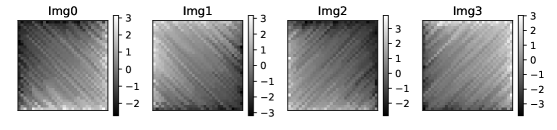
There is an important reason why we generate the synthetic dataset. Since most benchmark dataset contains very complex features, we cannot explicitly explain the internal logic of MLPs. As a comparison, the synthetic dataset only has four simple features. Therefore, we can clearly demonstrate the proposed probability space for a fully connected layer by simply visualizing the weights of the layer.

To classify the synthetic dataset, we specify the MLP as follows: (i) since each synthetic image is 32×3232\times 32, the input layer x{x} has M=1024M=1024 nodes, (ii) two hidden layers f1{f_{1}} and f2{f_{2}} have T=8T=8 and K=6K=6 neurons, respectively, and (iii) the output layer fY{f_{Y}} has L=4L=4 nodes. In addition, all the activation functions are chosen as ReLU σ(z)=max(0,z)\sigma(z)=\text{max}(0,z) unless otherwise specified.

Validation.
Refer to caption
Figure 8: The eight possible outcomes {𝝎t(1)}t=18\{\boldsymbol{\omega}^{(1)}_{t}\}_{t=1}^{8} represented by the learned weights of the eight neurons, where 𝝎t(1)={ωmt(1)}m=11024\boldsymbol{\omega}^{(1)}_{t}=\{\omega^{(1)}_{mt}\}_{m=1}^{1024}. All the weights {ωmt(1)}m=11024\{\omega^{(1)}_{mt}\}_{m=1}^{1024} are reshaped to 32×3232\times 32 dimension for visualizing the spatial structure.

To demonstrate (Ω,𝒯,QF)(\Omega,\mathcal{T},Q_{F}) for all the fully connected layers in the MLP={x;f1;f2;fY}\text{MLP}=\{{x;f_{1};f_{2};f_{Y}}\}, we only need to demonstrate (Ω1,𝒯,QF1)(\Omega_{1},\mathcal{T},Q_{F_{1}}) for the first layer f1{f_{1}}, because we derive (Ω,𝒯,QF)(\Omega,\mathcal{T},Q_{F}) for each layer in the back-forward direction based on the mathematical induction.
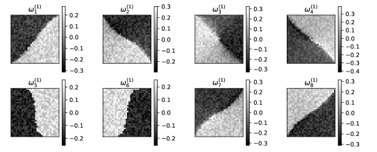
First, we demonstrate the sample space Ω1={𝝎t(1)}t=1T\Omega_{1}=\{\boldsymbol{\omega}^{(1)}_{t}\}_{t=1}^{T} for f1{f_{1}}. More specifically, we use the synthetic dataset to train the MLP 100 epochs (the training accuracy is 100%100\%) and visualize the learned weights of the eight neurons in f1{f_{1}}, i.e., 𝝎t(1)={ωmt(1)}m=11024,t[1,8],\boldsymbol{\omega}^{(1)}_{t}=\{\omega^{(1)}_{mt}\}_{m=1}^{1024},t\in[1,8], in Figure 8 . We can find that 𝝎t(1)\boldsymbol{\omega}^{(1)}_{t} can be regarded as a feature of the input. For example, 𝝎1(1)\boldsymbol{\omega}^{(1)}_{1} describes a feature indicating the difference along the secondary diagonal direction, because it has low magnitude at top-left positions and high magnitude at bottom-right positions. In addition, 𝝎1(1)\boldsymbol{\omega}^{(1)}_{1} is strongly related to Img0 in Figure 7, because the later has the same spatial feature. In the context of probability space, we define an experiment as inputting Img0 into f1{f_{1}}, thus 𝝎1(1)\boldsymbol{\omega}^{(1)}_{1} can be viewed as a possible outcome of the experiment. In addition, to keep consistent with the definition of outcome, we suppose 𝝎2(1)\boldsymbol{\omega}^{(1)}_{2} and 𝝎3(1)\boldsymbol{\omega}^{(1)}_{3} being mutually exclusive, because they have different weights at the same position, i.e., m,ωm2(1)ωm3(1)\forall m,\omega^{(1)}_{m2}\neq\omega^{(1)}_{m3}.

Table 1: The Gibbs probability of f1{f_{1}} given the synthetic images in Figure 7
𝝎𝟏(𝟏)\boldsymbol{\omega^{(1)}_{1}} 𝝎𝟐(𝟏)\boldsymbol{\omega^{(1)}_{2}} 𝝎𝟑(𝟏)\boldsymbol{\omega^{(1)}_{3}} 𝝎𝟒(𝟏)\boldsymbol{\omega^{(1)}_{4}} 𝝎𝟓(𝟏)\boldsymbol{\omega^{(1)}_{5}} 𝝎𝟔(𝟏)\boldsymbol{\omega^{(1)}_{6}} 𝝎𝟕(𝟏)\boldsymbol{\omega^{(1)}_{7}} 𝝎𝟖(𝟏)\boldsymbol{\omega^{(1)}_{8}}
g1t(x=Img0){g_{1t}(x=\text{\scriptsize Img0})} 27.53 8.98 -14.04 6.89 14.07 -22.24 25.85 -27.13
f1t(x=Img0){f_{1t}(x=\text{\scriptsize Img0})} 27.53 8.98 0.0 6.89 14.07 0.0 25.85 0.0
exp[f1t(x=Img0)]{\text{exp}[f_{1t}(x=\text{\scriptsize Img0})]} 9.03e+11 7.94e+03 1.0 1.0 1.28e+06 1.0 1.68e+11 1.0
QF1|X(𝝎𝒏(𝟏)|Img0){\scriptstyle Q_{F_{1}|{X}}(\boldsymbol{\omega^{(1)}_{n}}|\text{Img0})} 0.843 0.0 0.0 0.0 0.0 0.0 0.157 0.0
g1t(x=Img1){g_{1t}(x=\text{\scriptsize Img1})} -27.51 -9.81 12.96 -5.87 -13.05 21.68 -26.02 27.61
f1t(x=Img1){f_{1t}(x=\text{\scriptsize Img1})} 0.0 0.0 12.96 0.0 0.0 21.68 0.0 27.61
exp[f1t(x=Img1)]{\text{exp}[f_{1t}(x=\text{\scriptsize Img1})]} 1.0 1.0 4.25e+05 1.0 1.0 2.60e+09 1.0 9.79e+11
QF1|X(𝝎𝒕(𝟏)|Img1){\scriptstyle Q_{F_{1}|{X}}(\boldsymbol{\omega^{(1)}_{t}}|\text{Img1})} 0.0 0.0 0.0 0.0 0.0 0.003 0.0 0.997
g1t(x=Img2){g_{1t}(x=\text{\scriptsize Img2})} -2.69 26.28 24.64 -28.39 -20.44 12.23 10.13 -6.84
f1t(x=Img2){f_{1t}(x=\text{\scriptsize Img2})} 0.0 26.28 24.64 0.0 0.0 12.23 10.13 0.0
exp[f1t(x=Img2)]{\text{exp}[f_{1t}(x=\text{\scriptsize Img2})]} 1.0 2.58e+11 5.02e+10 1.0 1.0 2.04e+05 2.50e+04 1.0
QF1|X(𝝎𝒕(𝟏)|Img2){\scriptstyle Q_{F_{1}|{X}}(\boldsymbol{\omega^{(1)}_{t}}|\text{Img2})} 0.0 0.837 0.163 0.0 0.0 0.0 0.0 0.0
g1t(x=Img3){g_{1t}(x=\text{\scriptsize Img3})} 4.71 -26.20 -25.65 28.91 20.93 -13.18 -8.67 4.97
f1t(x=Img3){f_{1t}(x=\text{\scriptsize Img3})} 4.71 0.0 0.0 28.91 20.93 0.0 0.0 4.97
exp[f1t(x=Img3)]{\text{exp}[f_{1t}(x=\text{\scriptsize Img3})]} 1.11e+02 1.0 1.0 3.59e+12 1.22e+09 1.0 1.0 1.44e+02
QF1|X(𝝎𝒕(𝟏)|Img3){\scriptstyle Q_{F_{1}|{X}}(\boldsymbol{\omega^{(1)}_{t}}|\text{Img3})} 0.0 0.0 0.0 1.0 0.0 0.0 0.0 0.0
  • g1t(x)g_{1t}({x}) and f1t(x)f_{1t}({x}) denote the linear output and the activation, respectively, where g1t(x)=𝝎t(1),x+b1tg_{1t}({x})=\langle\boldsymbol{\omega}^{(1)}_{t},{x}\rangle+b_{1t} and f1t=σ1[g1t(x)]f_{1t}=\sigma_{1}[g_{1t}({x})].

Second, we demonstrate the Gibbs probability measure QF1Q_{F_{1}} for f1{f_{1}}. Based on Equation 33, we summarize QF1(𝝎t(1))Q_{F_{1}}(\boldsymbol{\omega}^{(1)}_{t}) given the four synthetic images (Figure 7) in Table 1, and find that QF1Q_{F_{1}} correctly measures the probability of the outcomes {𝝎t(1)}t=18\{\boldsymbol{\omega}^{(1)}_{t}\}_{t=1}^{8} occurring in the experiment based on the relation between 𝝎t(1)\boldsymbol{\omega}^{(1)}_{t} and x{x}. For example, 𝝎1(1)\boldsymbol{\omega}^{(1)}_{1} correctly describes the feature of Img0, thus it has the highest linear output and activation (g11(x)=27.53g_{11}({x})=27.53 and f11(x)=27.53f_{11}({x})=27.53), thereby QF|X(𝝎𝟏(𝟏)|Img0)=0.843Q_{F|{X}}(\boldsymbol{\omega^{(1)}_{1}}|\text{Img0})=0.843. As a comparison, since 𝝎8(1)\boldsymbol{\omega}^{(1)}_{8} oppositely describes the feature of Img0, it has the lowest linear output and activation (g18(x)=27.13g_{18}({x})=-27.13 and f18(x)=0.0f_{18}({x})=0.0), thereby QF|X(𝝎𝟖(𝟏)|Img0)=0.0Q_{F|{X}}(\boldsymbol{\omega^{(1)}_{8}}|\text{Img0})=0.0.

In summary, we demonstrate the probability space (Ω(\Omega, 𝒯,QF)\mathcal{T},Q_{F}) for a fully connected layer based on the synthetic dataset. The learned weights of neurons generate a sample space Ω\Omega consisting of multiple possible outcomes/features occurring in the input. The energy of each possible outcomes equals the negative activation of each neuron. The Gibbs function QFQ_{F} quantifies the probability of outcomes occurring in the input.

B.3 The equivalence between SGD and the first order approximation

If an arbitrary function f{f} is differentiable at point pN{p}^{*}\in{\mathbb{R}}^{N} and its differential is represented by the Jacobian matrix pf\nabla_{p}{f}, the first order approximation of f{f} near the point p{p} can be formulated as

f(p)f(p)=(pf)(pp)+o(pp),{f}({p})-{f}({p}^{*})=(\nabla_{{p}^{*}}{f})\cdot({p}-{p}^{*})+o(||{p}-{p}^{*}||), (34)

where o(pp)o(||{p}-{p}^{*}||) is a quantity that approaches zero much faster than pp||{p}-{p}^{*}|| approaches zero.

Based on the first order approximation [4], the activations in f2f_{2} and f1f_{1} in the MLP={x,f1,f2,fY}\text{MLP}=\{x,f_{1},f_{2},f_{Y}\} can be expressed as follows:

f2[f1,θj+1(2)]f2[f1,θj(2)]+(θj(2)f2)[θj+1(2)θj(2)]f1[x,θj+1(1)]f1[x,θj(1)]+(θj(1)f1)[θj+1(1)θj(1)],\begin{split}{f_{2}}[{f_{1}},{\theta}_{j+1}(2)]&\approx{f_{2}}[{f_{1}},{\theta}_{j}(2)]+(\nabla_{{\theta}_{j}(2)}{f_{2}})\cdot[{\theta}_{j+1}(2)-{\theta}_{j}(2)]\\ {f_{1}}[{x},{\theta}_{j+1}(1)]&\approx{f_{1}}[{x},{\theta}_{j}(1)]+(\nabla_{{\theta}_{j}(1)}{f_{1}})\cdot[{\theta}_{j+1}(1)-{\theta}_{j}(1)],\\ \end{split} (35)

where f2[f1,θj+1(2)]{f_{2}}[{f_{1}},{\theta}_{j+1}(2)] are the activations of the second hidden layer based on the parameters of f2f_{2} learned in the j+1j+1th iteration, i.e., θj+1(2){\theta}_{j+1}(2), given the activations of the first hidden layer, i.e., f1{f_{1}}. In addition, the definitions of f2[f1,θj(2)]{f_{2}}[{f_{1}},{\theta}_{j}(2)], f1(x,θj+1(1)){f_{1}}({x},{\theta}_{j+1}(1)), and f1(x,θj(1)){f_{1}}({x},{\theta}_{j}(1)) are the same as f2[f1,θj+1(2)]{f_{2}}[{f_{1}},{\theta}_{j+1}(2)].

Since f2={f2k=σ2(t=1Tωtk(2)f1t+b2k)}k=1K{f_{2}}=\{f_{2k}=\sigma_{2}(\sum_{t=1}^{T}\omega^{(2)}_{tk}\cdot f_{1t}+b_{2k})\}_{k=1}^{K} has KK neurons and each neuron has T+1T+1 parameters, namely θ(2)={ω1k(2);;ωTk(2);b2k}k=1K{\theta}(2)=\{\omega^{(2)}_{1k};\cdots;\omega^{(2)}_{Tk};b_{2k}\}_{k=1}^{K}, the dimension of θj(2)f2\nabla_{{\theta}_{j}(2)}{f_{2}} is equal to K×(T+1)K\times(T+1) and θj(2)f2\nabla_{{\theta}_{j}(2)}{f_{2}} can be expressed as

θj(2)f2=(σ2f2)[f1;1]T\begin{split}\nabla_{{\theta}_{j}(2)}{f_{2}}=(\nabla_{\sigma_{2}}{f_{2}})\cdot[{f_{1}};1]^{T}\end{split} (36)

where σ2f2=f2[f1,θt(2)]σ2\nabla_{\sigma_{2}}{f_{2}}=\frac{\partial{f_{2}}[{f_{1}},{\theta}_{t}(2)]}{\partial\sigma_{2}}. Substituting (σ2f2)[f1;1]T(\nabla_{\sigma_{2}}{f_{2}})\cdot[{f_{1}};1]^{T} for θj(2)f2\nabla_{{\theta}_{j}(2)}{f_{2}} in Equation 35, we derive

f2[f1,θj+1(2)]f2[f1,θj(2)]+(σ2f2)[f1;1]Tθj+1(2)(σ2f2)[f1;1]Tθj(2)\begin{split}{f_{2}}[{f_{1}},{\theta}_{j+1}(2)]\approx&{f_{2}}[{f_{1}},{\theta}_{j}(2)]+(\nabla_{\sigma_{2}}{f_{2}})\cdot[{f_{1}};1]^{T}\cdot{\theta}_{j+1}(2)-(\nabla_{\sigma_{2}}{f_{2}})\cdot[{f_{1}};1]^{T}\cdot{\theta}_{j}(2)\end{split} (37)

If we only consider a single neuron, e.g., f2kf_{2k}, we define θj+1(2k)=[ω1k(1);;ωTk(1);b2k]{\theta}_{j+1}(2k)=[\omega^{(1)}_{1k};\cdots;\omega^{(1)}_{Tk};b_{2k}] and θj(2k)=[ω1k(1);;ωTk(1);b2k]{\theta}_{j}(2k)=[\omega^{\prime(1)}_{1k};\cdots;\omega^{\prime(1)}_{Tk};b^{\prime}_{2k}], thus [f1;1]Tθj+1(2k)=t=1Tωtk(2)f1t+b2k[{f_{1}};1]^{T}\cdot{\theta}_{j+1}(2k)=\sum_{t=1}^{T}\omega^{(2)}_{tk}\cdot f_{1t}+b_{2k}. As a result, for a single neuron, Equation 37 can be expressed as

f2k[f1,θj+1(2k)](σ2f2k)[t=1Tωtk(2)f1t+b2k]Approximation+f2k[f1,θj(2k)](σ2f2k)[t=1Tωtk(2)f1t+b2k]Bias\begin{split}{f_{2k}}[{f_{1}},{\theta}_{j+1}(2k)]\approx\underbrace{(\nabla_{\sigma_{2}}f_{2k})\cdot[\sum_{t=1}^{T}\omega^{(2)}_{tk}\cdot f_{1t}+b_{2k}]}_{\text{Approximation}}+\underbrace{f_{2k}[{f_{1}},{\theta}_{j}(2k)]-(\nabla_{\sigma_{2}}f_{2k})\cdot[\sum_{t=1}^{T}\omega^{\prime(2)}_{tk}\cdot f_{1t}+b^{\prime}_{2k}]}_{\text{Bias}}\end{split} (38)

Equation 38 indicates that f2k[f1,θj+1(2k)]{f_{2k}}[{f_{1}},{\theta}_{j+1}(2k)] can be reformulated as two components: approximation and bias. Since σ2f2k=f2k[f1,θj(2)]σ2\nabla_{\sigma_{2}}f_{2k}=\frac{\partial f_{2k}[{f_{1}},{\theta}_{j}(2)]}{\partial\sigma_{2}} is only related to f1{f_{1}} and θj(2){\theta}_{j}(2), it can be regarded as a constant with respect to θj+1(2){\theta}_{j+1}(2). The bias component also does not contain any parameters in the (j+1)(j+1)th training iteration.

In summary, f2k(f1,θj+1(2k)){f_{2k}}({f_{1}},{\theta}_{j+1}(2k)) can be reformulated as

f2k(f1,θj+1(2k))C1[t=1Tωtk(2)f1t+b2k]+C2\begin{split}{f_{2k}}({f_{1}},{\theta}_{j+1}(2k))&\approx C_{1}\cdot[\sum_{t=1}^{T}\omega^{(2)}_{tk}\cdot f_{1t}+b_{2k}]+C_{2}\\ \end{split} (39)

where C1=σ2f2kC_{1}=\nabla_{\sigma_{2}}f_{2k} and C2=f2k(f1,θj(2k))(σ2f2k)[t=1Tωtk(2)f1t+b2k]C2=f_{2k}({f_{1}},{\theta}_{j}(2k))-(\nabla_{\sigma_{2}}f_{2k})\cdot[\sum_{t=1}^{T}\omega^{(2)}_{tk}\cdot f_{1t}+b^{*}_{2k}]. Similarly, the activations in the first hidden layer f1{f_{1}} also can be formulated as the approximation. To validate the approximation, we only need prove θj+1(2)θj(2){\theta}_{j+1}(2)-{\theta}_{j}(2) approaching zero, which can be guaranteed by SGD.

Given the MLP={x;f1;f2;fY}\text{MLP}=\{{x;f_{1};f_{2};f_{Y}}\} and the empirical risk ^𝒮(h)\hat{\mathcal{L}}^{\ell}_{\mathcal{S}}(h), SGD aims to optimize the parameters of the MLP through minimizing ^𝒮(h)\hat{\mathcal{L}}^{\ell}_{\mathcal{S}}(h) [35].

θt+1=θtαθt^𝒮(h),{\theta}_{t+1}={\theta}_{t}-\alpha\nabla_{\theta_{t}}\hat{\mathcal{L}}^{\ell}_{\mathcal{S}}(h), (40)

where θt^𝒮(h)\nabla_{\theta_{t}}\hat{\mathcal{L}}^{\ell}_{\mathcal{S}}(h) denotes the Jacobian matrix of ^𝒮(h)\hat{\mathcal{L}}^{\ell}_{\mathcal{S}}(h) with respect to θt{\theta}_{t} at the ttth iteration, and α>0\alpha>0 denotes the learning rate. Since the functions of all the layers are differentiable, the Jacobian matrix of ^𝒮(h)\hat{\mathcal{L}}^{\ell}_{\mathcal{S}}(h) with respect to the parameters of the iith hidden layer, i.e., θ(i)^𝒮(h)\nabla_{\theta(i)}\hat{\mathcal{L}}^{\ell}_{\mathcal{S}}(h), can be expressed as

θ(y)^𝒮(h)=fY^𝒮(h)θYfYθ(2)^𝒮(h)=fY^𝒮(h)f2fYθ2f2θ(1)^𝒮(h)=fY^𝒮(h)f2fYf1f2θ1f1,\begin{split}\nabla_{{\theta}(y)}\hat{\mathcal{L}}^{\ell}_{\mathcal{S}}(h)&=\nabla_{{f_{Y}}}\hat{\mathcal{L}}^{\ell}_{\mathcal{S}}(h)\nabla_{{\theta_{Y}}}f_{Y}\\ \nabla_{{\theta}(2)}\hat{\mathcal{L}}^{\ell}_{\mathcal{S}}(h)&=\nabla_{{f_{Y}}}\hat{\mathcal{L}}^{\ell}_{\mathcal{S}}(h)\nabla_{f_{2}}f_{Y}\nabla_{\theta_{2}}f_{2}\\ \nabla_{{\theta}(1)}\hat{\mathcal{L}}^{\ell}_{\mathcal{S}}(h)&=\nabla_{{f_{Y}}}\hat{\mathcal{L}}^{\ell}_{\mathcal{S}}(h)\nabla_{{f_{2}}}f_{Y}\nabla_{{f_{1}}}f_{2}\nabla_{\theta_{1}}f_{1},\end{split} (41)

where θ(i){\theta}(i) denote the parameters of the iith layer. Equation 40 and 41 indicate that θ(i){\theta}(i) can be learned as

θt+1(i)=θt(i)α[θt(i)^𝒮(h)].{\theta}_{t+1}(i)={\theta}_{t}(i)-\alpha[\nabla_{\theta_{t}(i)}\hat{\mathcal{L}}^{\ell}_{\mathcal{S}}(h)]. (42)

Table 2 summarizes SGD training procedure for the MLP shown in Figure 6.

SGD minimizing ^𝒮(h)\hat{\mathcal{L}}^{\ell}_{\mathcal{S}}(h) indicates θt(i)^𝒮(h)\nabla_{\theta_{t}(i)}\hat{\mathcal{L}}^{\ell}_{\mathcal{S}}(h) converging to zero, thereby θt+1(i)θt(i){\theta}_{t+1}(i)-{\theta}_{t}(i) converging to zero.

Table 2: One iteration of SGD training procedure for the MLP
Layer Gradients θ(i)^𝒮(h)\nabla_{\theta(i)}\hat{\mathcal{L}}^{\ell}_{\mathcal{S}}(h) Parameters Activations
fY{f_{Y}} 𝜽(y)^𝒮(h){\scriptstyle\nabla_{\boldsymbol{\theta}(y)}\hat{\mathcal{L}}^{\ell}_{\mathcal{S}}(h)} \downarrow θt+1(Y)=θt+1(Y)α[θ(y)^𝒮(h)]{\scriptstyle{\theta}_{t+1}(Y)={\theta}_{t+1}(Y)-\alpha[\nabla_{{\theta}(y)}\hat{\mathcal{L}}^{\ell}_{\mathcal{S}}(h)]} \uparrow fY(f2,θt+1(Y)){\scriptstyle{f_{Y}}({f_{2}},{\theta}_{t+1}(Y))} \uparrow
f2{f_{2}} 𝜽(2)^𝒮(h){\scriptstyle\nabla_{\boldsymbol{\theta}(2)}\hat{\mathcal{L}}^{\ell}_{\mathcal{S}}(h)} \downarrow θt+1(2)=θt+1(2)α[θ(2)^𝒮(h)]{\scriptstyle{\theta}_{t+1}(2)={\theta}_{t+1}(2)-\alpha[\nabla_{{\theta}(2)}\hat{\mathcal{L}}^{\ell}_{\mathcal{S}}(h)]} \uparrow f2(f1,θt+1(2)){\scriptstyle{f_{2}}({f_{1}},{\theta}_{t+1}(2))} \uparrow
f1{f_{1}} 𝜽(1)^𝒮(h){\scriptstyle\nabla_{\boldsymbol{\theta}(1)}\hat{\mathcal{L}}^{\ell}_{\mathcal{S}}(h)} \downarrow θt+1(1)=θt+1(1)α[θ(1)^𝒮(h)]{\scriptstyle{\theta}_{t+1}(1)={\theta}_{t+1}(1)-\alpha[\nabla_{{\theta}(1)}\hat{\mathcal{L}}^{\ell}_{\mathcal{S}}(h)]} \uparrow f1(x,θt+1(1)){\scriptstyle{f_{1}}({x},{\theta}_{t+1}(1))} \uparrow
x{x}
  • The up-arrow and down-arrow indicate the order of gradients and parameters(activations) update, respectively.

C The derivation of the marginal distribution Q(FY|X)Q(F_{Y}|{X})

Since the entire architecture of the MLP={x;f1;f2;fY}\text{MLP}=\{{x;f_{1};f_{2};f_{Y}}\} in Figure 6 corresponds to a joint distribution Q(FY;F2;F1|X)=Q(FY|F2)P(F2|F1)P(F1|X)Q(F_{Y};F_{2};F_{1}|{X})=Q(F_{Y}|F_{2})P(F_{2}|F_{1})P(F_{1}|{X}), the marginal distribution Q(FY|X)Q(F_{Y}|{X}) can be formulated as

QFY|X(l|xi)=k=1Kt=1TQ(FY=l,F2=k,F1=t|X=xi)=k=1KQFY|F2(l|k)t=1TQF2|F1(k|t)QF1|X(t|xi).\begin{split}Q_{F_{Y}|X}(l|{x}_{i})&=\sum_{k=1}^{K}\sum_{t=1}^{T}Q(F_{Y}=l,F_{2}=k,F_{1}=t|X={x}_{i})\\ &=\sum_{k=1}^{K}Q_{F_{Y}|F_{2}}(l|k)\sum_{t=1}^{T}Q_{F_{2}|F_{1}}(k|t)Q_{F_{1}|X}(t|{x}_{i}).\\ \end{split} (43)

Based on the definition of the Gibbs probability measure (Equation 6), we have

QF1|X(t|xi)=1ZF1exp(f1t)=1ZF1exp[σ1(𝝎t(1),xi)],Q_{F_{1}|X}(t|{x}_{i})=\frac{1}{Z_{{F_{1}}}}\text{exp}(f_{1t})=\frac{1}{Z_{{F_{1}}}}\text{exp}[\sigma_{1}(\langle{\boldsymbol{\omega}^{\prime}}^{(1)}_{t},{x}^{\prime}_{i}\rangle)], (44)

where 𝝎t(1)=[𝝎t(1),b1n]{\boldsymbol{\omega}^{\prime}}^{(1)}_{t}=[{\boldsymbol{\omega}}^{(1)}_{t},b_{1n}] and xi=[xi,1]{x}^{\prime}_{i}=[{x}_{i},1], i.e., 𝝎t(1),xi=𝝎t(1),xi+b1n\langle{\boldsymbol{\omega}^{\prime}}^{(1)}_{t},{x}^{\prime}_{i}\rangle=\langle{\boldsymbol{\omega}}^{(1)}_{t},{x}_{i}\rangle+b_{1n}.

Similarly, we have

QF2|F1(k|t)=1ZF2exp(f2k)=1ZF2exp[σ2(𝝎k(2),f1)],Q_{F_{2}|F_{1}}(k|t)=\frac{1}{Z_{{F_{2}}}}\text{exp}(f_{2k})=\frac{1}{Z_{{F_{2}}}}\text{exp}[\sigma_{2}(\langle{\boldsymbol{\omega}^{\prime}}^{(2)}_{k},{f}^{\prime}_{1}\rangle)], (45)

where f1={f1t}t=1T={σ1(𝝎t(1),xi)}t=1T{f}_{1}=\{f_{1t}\}_{t=1}^{T}=\{\sigma_{1}(\langle{\boldsymbol{\omega}^{\prime}}^{(1)}_{t},{x}^{\prime}_{i}\rangle)\}_{t=1}^{T}, 𝝎k(2)=[𝝎k(2),b2k]{\boldsymbol{\omega}^{\prime}}^{(2)}_{k}=[{\boldsymbol{\omega}}^{(2)}_{k},b_{2k}] and f1=[f1,1]{f}^{\prime}_{1}=[{f}_{1},1], i.e., 𝝎k(2),f1=𝝎k(2),f1+b2k\langle{\boldsymbol{\omega}^{\prime}}^{(2)}_{k},{f}^{\prime}_{1}\rangle=\langle{\boldsymbol{\omega}}^{(2)}_{k},{f}_{1}\rangle+b_{2k}. Therefore, we have

t=1TQF2|F1(k|t)QF1|X(t|xi)=1ZF21ZF1t=1Texp[σ2(𝝎k(2),f1)]exp[σ1(𝝎t(1),xi)].\begin{split}\sum_{t=1}^{T}Q_{F_{2}|F_{1}}(k|t)Q_{F_{1}|X}(t|{x}_{i})=\frac{1}{Z_{{F_{2}}}}\frac{1}{Z_{{F_{1}}}}\sum_{t=1}^{T}\text{exp}[\sigma_{2}(\langle{\boldsymbol{\omega}^{\prime}}^{(2)}_{k},{f}^{\prime}_{1}\rangle)]\text{exp}[\sigma_{1}(\langle{\boldsymbol{\omega}^{\prime}}^{(1)}_{t},{x}^{\prime}_{i}\rangle)].\\ \end{split} (46)

Since 𝝎k(2),f1=𝝎k(2),f1+b2k=t=1Tωkt(2)f1t+b2k\langle{\boldsymbol{\omega}^{\prime}}^{(2)}_{k},{f}^{\prime}_{1}\rangle=\langle{\boldsymbol{\omega}}^{(2)}_{k},{f}_{1}\rangle+b_{2k}=\sum_{t=1}^{T}\omega^{(2)}_{kt}f_{1t}+b_{2k} is a constant with respect to tt, we have

t=1TQF2|F1(k|t)QF1|X(t|xi)=1ZF21ZF1exp[σ2(𝝎k(2),f1)]t=1Texp[σ1(𝝎t(1),xi)].\sum_{t=1}^{T}Q_{F_{2}|F_{1}}(k|t)Q_{F_{1}|X}(t|{x}_{i})=\frac{1}{Z_{{F_{2}}}}\frac{1}{Z_{{F_{1}}}}\text{exp}[\sigma_{2}(\langle{\boldsymbol{\omega}^{\prime}}^{(2)}_{k},{f}^{\prime}_{1}\rangle)]\sum_{t=1}^{T}\text{exp}[\sigma_{1}(\langle{\boldsymbol{\omega}^{\prime}}^{(1)}_{t},{x}^{\prime}_{i}\rangle)]. (47)

In addition, t=1Texp[σ1(𝝎t(1),xi)]=ZF1\sum_{t=1}^{T}\text{exp}[\sigma_{1}(\langle{\boldsymbol{\omega}^{\prime}}^{(1)}_{t},{x}^{\prime}_{i}\rangle)]=Z_{F_{1}}, thus we have

t=1TQF2|F1(k|t)QF1|X(t|xi)=1ZF2exp[σ2(𝝎k(2),f1)].\sum_{t=1}^{T}Q_{F_{2}|F_{1}}(k|t)Q_{F_{1}|X}(t|{x}_{i})=\frac{1}{Z_{{F_{2}}}}\text{exp}[\sigma_{2}(\langle{\boldsymbol{\omega}^{\prime}}^{(2)}_{k},{f}^{\prime}_{1}\rangle)]. (48)

Therefore, we can simplify QFY|X(l|xi)Q_{F_{Y}|X}(l|{x}_{i}) as

QFY|X(l|xi)=k=1KQFY|F2(l|k)t=1TQF2|F1(k|t)QF1|X(t|xi)=k=1KQFY|F2(l|k)1ZF2exp[σ2(𝝎k(2),f1)].\begin{split}Q_{F_{Y}|X}(l|{x}_{i})&=\sum_{k=1}^{K}Q_{F_{Y}|F_{2}}(l|k)\sum_{t=1}^{T}Q_{F_{2}|F_{1}}(k|t)Q_{F_{1}|X}(t|{x}_{i})\\ &=\sum_{k=1}^{K}Q_{F_{Y}|F_{2}}(l|k)\frac{1}{Z_{{F_{2}}}}\text{exp}[\sigma_{2}(\langle{\boldsymbol{\omega}^{\prime}}^{(2)}_{k},{f}^{\prime}_{1}\rangle)].\\ \end{split} (49)

Similarly, since QFY|F2(l|k)=1ZFYexp[σ3(𝝎l(3),f2+byl)]Q_{F_{Y}|F_{2}}(l|k)=\frac{1}{Z_{{F_{Y}}}}\text{exp}[\sigma_{3}(\langle{\boldsymbol{\omega}}^{(3)}_{l},{f}_{2}\rangle+b_{yl})] and 𝝎l(3),f2=k=1Kωlk(3)f2k\langle{\boldsymbol{\omega}}^{(3)}_{l},{f}_{2}\rangle=\sum_{k=1}^{K}\omega^{(3)}_{lk}f_{2k} is also a constant with respect to kk, we can derive

QFY|X(l|xi)=QFY|F2(l|k)=1ZFYexp[σ3(𝝎l(3),f2+byl)].\begin{split}Q_{F_{Y}|X}(l|{x}_{i})=Q_{F_{Y}|F_{2}}(l|k)=\frac{1}{Z_{F_{Y}}}\text{exp}[\sigma_{3}(\langle{\boldsymbol{\omega}}^{(3)}_{l},{f}_{2}\rangle+b_{yl})].\end{split} (50)

In addition, since f2={f2k}k=1K={σ2(𝝎k(2),f1+b2k)}k=1K{f}_{2}=\{f_{2k}\}_{k=1}^{K}=\{\sigma_{2}(\langle{\boldsymbol{\omega}}^{(2)}_{k},{f}_{1}\rangle+b_{2k})\}_{k=1}^{K}, we can extend QFY|X(l|xi)Q_{F_{Y}|X}(l|{x}_{i}) as

QFY|X(l|xi)=QFY|F2(l|k)=1ZFYexp[σ3(𝝎l(3),f2+byl)]=1ZFYexp[σ3(𝝎l(3),(σ2(𝝎1(2),f1+b21)σ2(𝝎K(2),f1+b2K))+byl)].\begin{split}Q_{F_{Y}|X}(l|{x}_{i})&=Q_{F_{Y}|F_{2}}(l|k)=\frac{1}{Z_{F_{Y}}}\text{exp}[\sigma_{3}(\langle{\boldsymbol{\omega}}^{(3)}_{l},{f}_{2}\rangle+b_{yl})]\\ &=\frac{1}{Z_{F_{Y}}}\text{exp}[\sigma_{3}(\langle{\boldsymbol{\omega}}^{(3)}_{l},\left(\begin{array}[]{c}\sigma_{2}(\langle{\boldsymbol{\omega}}^{(2)}_{1},{f}_{1}\rangle+b_{21})\\ \vdots\\ \sigma_{2}(\langle{\boldsymbol{\omega}}^{(2)}_{K},{f}_{1}\rangle+b_{2K})\end{array}\right)\rangle+b_{yl})].\end{split} (51)

Since f1={f1t}t=1T={σ1(𝝎t(1),xi+b1n)}t=1T{f}_{1}=\{f_{1t}\}_{t=1}^{T}=\{\sigma_{1}(\langle{\boldsymbol{\omega}}^{(1)}_{t},{x}_{i}\rangle+b_{1n})\}_{t=1}^{T}, we can further extend QFY|X(l|xi)Q_{F_{Y}|X}(l|{x}_{i}) as

QFY|X(l|xi)=1ZFYexp[σ3(𝝎l(3),(σ2(𝝎1(2),(σ1(𝝎1(1),xi+b11)σ1(𝝎1(1),xi+b11))+b21)σ2(𝝎K(2),(σ1(𝝎T(1),xi+b1T)σ1(𝝎T(1),xi+b1T))+b2K))+byl)].=1ZMLP(xi)exp[fyl(f2(f1(xi)))]\begin{split}Q_{F_{Y}|X}(l|{x}_{i})&=\frac{1}{Z_{F_{Y}}}\text{exp}[\sigma_{3}(\langle{\boldsymbol{\omega}}^{(3)}_{l},\left(\begin{array}[]{c}\sigma_{2}(\langle{\boldsymbol{\omega}}^{(2)}_{1},\left(\begin{array}[]{c}\sigma_{1}(\langle{\boldsymbol{\omega}}^{(1)}_{1},{x}_{i}\rangle+b_{11})\\ \vdots\\ \sigma_{1}(\langle{\boldsymbol{\omega}}^{(1)}_{1},{x}_{i}\rangle+b_{11})\end{array}\right)\rangle+b_{21})\\ \vdots\\ \sigma_{2}(\langle{\boldsymbol{\omega}}^{(2)}_{K},\left(\begin{array}[]{c}\sigma_{1}(\langle{\boldsymbol{\omega}}^{(1)}_{T},{x}_{i}\rangle+b_{1T})\\ \vdots\\ \sigma_{1}(\langle{\boldsymbol{\omega}}^{(1)}_{T},{x}_{i}\rangle+b_{1T})\end{array}\right)\rangle+b_{2K})\end{array}\right)\rangle+b_{yl})].\\ &=\frac{1}{Z_{\text{MLP}}(x_{i})}\text{exp}[{f_{yl}(f_{2}(f_{1}({x}_{i})))}]\end{split} (52)

Overall, we prove that QFY|X(l|xi)Q_{F_{Y}|X}(l|{x}_{i}) is also a Gibbs distribution and it can be expressed as

QFY|X(l|xi)=1ZMLP(xi)exp[fyl(f2(f1(xi)))].Q_{F_{Y}|X}(l|{x}_{i})=\frac{1}{Z_{\text{MLP}}({x}_{i})}\text{exp}[f_{yl}(f_{2}(f_{1}({x}_{i})))]. (53)

where Eyl(xi)=fyl(f2(f1(xi)))E_{yl}(x_{i})=-f_{yl}(f_{2}(f_{1}({x}_{i}))) is the energy function of l𝒴l\in\mathcal{Y} given xix_{i} and the partition function ZMLP(xi)=l=1Lk=1Kt=1TQ(FY,F2,F1|X=xi)=l=1Lexp[fyl(f2(f1(xi)))]Z_{\text{MLP}}({x}_{i})=\sum_{l=1}^{L}\sum_{k=1}^{K}\sum_{t=1}^{T}Q(F_{Y},F_{2},F_{1}|X=x_{i})=\sum_{l=1}^{L}\text{exp}[f_{yl}(f_{2}(f_{1}({x}_{i})))].

D KL[P(FY|X,Y)||Q(FY|X)]\text{KL}[P^{*}(F_{Y}|X,Y)||Q(F_{Y}|X)] approachs KL[Q(FY|X)||P(FY|X,Y)]\text{KL}[Q(F_{Y}|X)||P^{*}(F_{Y}|X,Y)]

This appendix demonstrates KL[P(FY|X,Y)||Q(FY|X)]KL[Q(FY|X)||P(FY|X,Y)]\text{KL}[P^{*}(F_{Y}|X,Y)||Q(F_{Y}|X)]\rightarrow\text{KL}[Q(F_{Y}|X)||P^{*}(F_{Y}|X,Y)] because d0d\rightarrow 0 during minimizing ^𝒮(h)\hat{\mathcal{L}}^{\ell}_{\mathcal{S}}(h).

Recall d=KL[P(FY|X,Y)||Q(FY|X)]KL[Q(FY|X)||P(FY|X,Y)]d=\text{KL}[P^{*}(F_{Y}|X,Y)||Q(F_{Y}|X)]-\text{KL}[Q(F_{Y}|X)||P^{*}(F_{Y}|X,Y)], the property of cross entropy, i.e., KL[P||Q]=H(P,Q)H(P)\text{KL}[P||Q]=H(P,Q)-H(P), allows us to derive

d=H[P(FY|X,Y),Q(FY|X)]H[P(FY|X,Y)]KL[P(FY|X,Y)||Q(FY|X)]{H[Q(FY|X),P(FY|X,Y)]H[Q(FY|X)]}KL[Q(FY|X)||P(FY|X,Y)].d=\underbrace{H[P^{*}(F_{Y}|X,Y),Q(F_{Y}|X)]-H[P^{*}(F_{Y}|X,Y)]}_{\text{KL}[P^{*}(F_{Y}|X,Y)||Q(F_{Y}|X)]}-\underbrace{\{H[Q(F_{Y}|X),P^{*}(F_{Y}|X,Y)]-H[Q(F_{Y}|X)]\}}_{\text{KL}[Q(F_{Y}|X)||P^{*}(F_{Y}|X,Y)]}. (54)

where H(P)H(P) denotes the entropy of PP. Since P(FY|X,Y)P^{*}(F_{Y}|X,Y) is one-hot, namely that if l=yil=y_{i}, then PFY|X,Y(l|xi,yi)=1P^{*}_{F_{Y}|X,Y}(l|x_{i},y_{i})=1, otherwise PFY|X,Y(l|xi,yi)=0P^{*}_{F_{Y}|X,Y}(l|x_{i},y_{i})=0, we have

H[P(FY|X,Y)]=0,H[P(FY|X,Y),Q(FY|X)]=logQFY|X(yi|xi).\begin{split}H[P^{*}(F_{Y}|X,Y)]&=0,\\ H[P^{*}(F_{Y}|X,Y),Q(F_{Y}|X)]&=-\text{log}Q_{F_{Y}|X}(y_{i}|x_{i}).\end{split} (55)

Therefore, we can simplify dd as

d=logQFY|X(yi|xi)+l=1LQFY|X(l|xi)logPFY|X,Y(l|xi,yi)+H[Q(FY|X)].d=-\text{log}Q_{F_{Y}|X}(y_{i}|x_{i})+\sum_{l=1}^{L}Q_{F_{Y}|X}(l|x_{i})\text{log}P^{*}_{F_{Y}|X,Y}(l|x_{i},y_{i})+H[Q(F_{Y}|X)]. (56)

PFY|X,Y(l|xi,yi)=0P^{*}_{F_{Y}|X,Y}(l|x_{i},y_{i})=0 induces logPFY|X,Y(l|xi,yi)=\text{log}P^{*}_{F_{Y}|X,Y}(l|x_{i},y_{i})=-\infty. To guarantee dd is a valid value, we relax P(FY|X,Y)P^{*}(F_{Y}|X,Y) as

P^FY|X,Y(l|xi,yi)={1(L1)εifl=yiεiflyi\hat{P}^{*}_{F_{Y}|X,Y}(l|x_{i},y_{i})=\left\{\begin{array}[]{rcl}1-(L-1)\varepsilon&\text{if}&l=y_{i}\\ \varepsilon&\text{if}&l\neq y_{i}\end{array}\right. (57)

where ε\varepsilon is a small positive value. As a result, we have

d=logQFY|X(yi|xi)+[1QFY|X(yi|xi)](L1)logε+H[Q(FY|X=xi)]+QFY|X(yi|xi)log[1(L1)ε].\begin{split}d=&-\text{log}Q_{F_{Y}|X}(y_{i}|x_{i})+[1-Q_{F_{Y}|X}(y_{i}|x_{i})](L-1)\text{log}\varepsilon+H[Q(F_{Y}|X=x_{i})]\\ &+Q_{F_{Y}|X}(y_{i}|x_{i})\text{log}[1-(L-1)\varepsilon].\end{split} (58)

Corollary 1 indicates that minimizing ^𝒮(h)\hat{\mathcal{L}}^{\ell}_{\mathcal{S}}(h) is equivalent to maximizing i=1nlogQFY|X(yi|xi)\sum_{i=1}^{n}\text{log}Q_{F_{Y}|X}(y_{i}|x_{i}). Since QFY|X(yi|xi)[0,1]Q_{F_{Y}|X}(y_{i}|x_{i})\in[0,1], maximizing i=1nlogQFY|X(yi|xi)\sum_{i=1}^{n}\text{log}Q_{F_{Y}|X}(y_{i}|x_{i}) makes QFY|X(yi|xi)Q_{F_{Y}|X}(y_{i}|x_{i}) to approach 1. As a result, logQFY|X(yi|xi)\text{log}Q_{F_{Y}|X}(y_{i}|x_{i}), [1QFY|X(yi|xi)](L1)logε[1-Q_{F_{Y}|X}(y_{i}|x_{i})](L-1)\text{log}\varepsilon, and H[Q(FY|X=xi)]H[Q(F_{Y}|X=x_{i})] approach 0. In addition, we have limε0QFY|X(yi|xi)log[1(L1)ε]=0\underset{\varepsilon\rightarrow 0}{\text{lim}}Q_{F_{Y}|X}(y_{i}|x_{i})\text{log}[1-(L-1)\varepsilon]=0. In summary, dd converges to 0 when minimizing ^𝒮(h)\hat{\mathcal{L}}^{\ell}_{\mathcal{S}}(h).

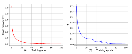
Moreover, we train the MLP1 designed in Section 5 on the MNIST dataset and visualize the variation of the cross entropy loss and dd during 100 epochs in Figure 9. We can observe that dd shows a similar decreasing trend as the cross entropy loss and dd converges to zero when the cross entropy loss approaches zero. Since dd converges to zero, KL[P(FY|X,Y)||Q(FY|X)]KL[Q(FY|X)||P(FY|X,Y)]\text{KL}[P^{*}(F_{Y}|X,Y)||Q(F_{Y}|X)]\rightarrow\text{KL}[Q(F_{Y}|X)||P^{*}(F_{Y}|X,Y)] during minimizing ^𝒮(h)\hat{\mathcal{L}}^{\ell}_{\mathcal{S}}(h).

Refer to caption
Figure 9: (A) and (B) show the variations of the cross entropy loss and dd during 100 training epochs, respectively.

E The derivation of the ELBO from Bayesian variational inference

Given the samples 𝒮\mathcal{S}, the MLP={x;f1;f2;fY}\text{MLP}=\{{x;f_{1};f_{2};f_{Y}}\}, and the cross entropy loss ^𝒮(h)\hat{\mathcal{L}}^{\ell}_{\mathcal{S}}(h), recall the corresponding Bayesian variational inference (Equation 17) as

KL[Q𝒮x(FY|X)||P𝒮(FY|X,Y)]=𝑬Q(FY|X)logQ𝒮x(FY|X)𝑬Q(FY|X)logP𝒮(FY|X,Y).\text{KL}[{\scriptstyle Q_{\mathcal{S}_{x}}(F_{Y}|X)}||{\scriptstyle P^{*}_{\mathcal{S}}(F_{Y}|X,Y)}]=\underset{Q(F_{Y}|X)}{\boldsymbol{E}}\text{log}{\scriptstyle Q_{\mathcal{S}_{x}}(F_{Y}|X)}-\underset{Q(F_{Y}|X)}{\boldsymbol{E}}\text{log}{\scriptstyle P^{*}_{\mathcal{S}}(F_{Y}|X,Y)}. (59)

Since P𝒮(FY|X,Y)=P𝒮(FY,Y|X)/P𝒮(Y|X)P^{*}_{\mathcal{S}}(F_{Y}|X,Y)=P^{*}_{\mathcal{S}}(F_{Y},Y|X)/P_{\mathcal{S}}(Y|X), we have

KL[Q𝒮x(FY|X)||P𝒮(FY|X,Y)]=𝑬Q(FY|X)logQ𝒮x(FY|X)𝑬Q(FY|X)[logP𝒮(FY,Y|X)logP𝒮(Y|X)].\text{KL}[{\scriptstyle Q_{\mathcal{S}_{x}}(F_{Y}|X)}||{\scriptstyle P^{*}_{\mathcal{S}}(F_{Y}|X,Y)}]=\underset{Q(F_{Y}|X)}{\boldsymbol{E}}\text{log}{\scriptstyle Q_{\mathcal{S}_{x}}(F_{Y}|X)}-\underset{Q(F_{Y}|X)}{\boldsymbol{E}}[\text{log}{\scriptstyle P^{*}_{\mathcal{S}}(F_{Y},Y|X)}-\text{log}{\scriptstyle P_{\mathcal{S}}(Y|X)}]. (60)

Since logP𝒮(Y|X)\text{log}P_{\mathcal{S}}(Y|X) is constant with respect to Q(FY|X)Q(F_{Y}|X), we have

KL[Q𝒮x(FY|X)||P𝒮(FY|X,Y)]=𝑬Q(FY|X)logQ𝒮x(FY|X)𝑬Q(FY|X)logP𝒮(FY,Y|X)+logP𝒮(Y|X).\text{KL}[{\scriptstyle Q_{\mathcal{S}_{x}}(F_{Y}|X)}||{\scriptstyle P^{*}_{\mathcal{S}}(F_{Y}|X,Y)}]=\underset{Q(F_{Y}|X)}{\boldsymbol{E}}\text{log}{\scriptstyle Q_{\mathcal{S}_{x}}(F_{Y}|X)}-\underset{Q(F_{Y}|X)}{\boldsymbol{E}}\text{log}{\scriptstyle P^{*}_{\mathcal{S}}(F_{Y},Y|X)}+\text{log}{\scriptstyle P_{\mathcal{S}}(Y|X)}. (61)

Since P𝒮(FY,Y|X)=P𝒮(Y|FY,X)P𝒮x(FY|X)P^{*}_{\mathcal{S}}(F_{Y},Y|X)=P_{\mathcal{S}}(Y|F_{Y},X)P^{*}_{\mathcal{S}_{x}}(F_{Y}|X), we have

KL[Q𝒮x(FY|X)||P𝒮(FY|X,Y)]=𝑬Q(FY|X)logQ𝒮x(FY|X)𝑬Q(FY|X)logP𝒮x(FY|X)𝑬Q(FY|X)logP𝒮(Y|FY,X)+logP𝒮(Y|X).\begin{split}\text{KL}[{\scriptstyle Q_{\mathcal{S}_{x}}(F_{Y}|X)}||{\scriptstyle P^{*}_{\mathcal{S}}(F_{Y}|X,Y)}]=&\underset{Q(F_{Y}|X)}{\boldsymbol{E}}\text{log}{\scriptstyle Q_{\mathcal{S}_{x}}(F_{Y}|X)}-\underset{Q(F_{Y}|X)}{\boldsymbol{E}}\text{log}{\scriptstyle P^{*}_{\mathcal{S}_{x}}(F_{Y}|X)}-\underset{Q(F_{Y}|X)}{\boldsymbol{E}}\text{log}{\scriptstyle P_{\mathcal{S}}(Y|F_{Y},X)}\\ &+\text{log}{\scriptstyle P_{\mathcal{S}}(Y|X)}.\end{split} (62)

Since 𝑬Q(FY|X)logQ𝒮x(FY|X)𝑬Q(FY|X)logP𝒮x(FY|X)=KL[Q𝒮x(FY|X)||P𝒮x(FY|X)]\underset{Q(F_{Y}|X)}{\boldsymbol{E}}\text{log}{\scriptstyle Q_{\mathcal{S}_{x}}(F_{Y}|X)}-\underset{Q(F_{Y}|X)}{\boldsymbol{E}}\text{log}{\scriptstyle P^{*}_{\mathcal{S}_{x}}(F_{Y}|X)}=\text{KL}[{\scriptstyle Q_{\mathcal{S}_{x}}(F_{Y}|X)}||{\scriptstyle P^{*}_{\mathcal{S}_{x}}(F_{Y}|X)}], we have

KL[Q𝒮x(FY|X)||P𝒮(FY|X,Y)]=KL[Q𝒮x(FY|X)||P𝒮x(FY|X)]𝑬Q(FY|X)logP𝒮(Y|FY,X)+logP𝒮(Y|X).\begin{split}\text{KL}[{\scriptstyle Q_{\mathcal{S}_{x}}(F_{Y}|X)}||{\scriptstyle P^{*}_{\mathcal{S}}(F_{Y}|X,Y)}]=\text{KL}[{\scriptstyle Q_{\mathcal{S}_{x}}(F_{Y}|X)}||{\scriptstyle P^{*}_{\mathcal{S}_{x}}(F_{Y}|X)}]-\underset{Q(F_{Y}|X)}{\boldsymbol{E}}\text{log}{\scriptstyle P_{\mathcal{S}}(Y|F_{Y},X)}+\text{log}{\scriptstyle P_{\mathcal{S}}(Y|X)}.\end{split} (63)

Finally, we can derive the ELBO as

logP𝒮(Y|X)=𝑬Q(FY|X)logP𝒮(Y|FY,X)KL[Q𝒮x(FY|X)||P𝒮x(FY|X)]ELBO+KL[Q𝒮x(FY|X)||P𝒮(FY|X,Y)],\text{log}P_{\mathcal{S}}(Y|X)=\underbrace{\underset{Q(F_{Y}|X)}{\boldsymbol{E}}\text{log}{\scriptstyle P_{\mathcal{S}}(Y|F_{Y},X)}-\text{KL}[{\scriptstyle Q_{\mathcal{S}_{x}}(F_{Y}|X)}||{\scriptstyle P^{*}_{\mathcal{S}_{x}}(F_{Y}|X)}]}_{\text{ELBO}}+\text{KL}[{\scriptstyle Q_{\mathcal{S}_{x}}(F_{Y}|X)}||{\scriptstyle P^{*}_{\mathcal{S}}(F_{Y}|X,Y)}], (64)

where P𝒮(Y|X)=i=1nP(Y=yi|X=xi)P_{\mathcal{S}}(Y|X)=\prod_{i=1}^{n}P(Y=y_{i}|X=x_{i}), P𝒮(Y|FY,X)=i=1nP(Y=yi|FY,X=xi)P_{\mathcal{S}}(Y|F_{Y},X)=\prod_{i=1}^{n}P(Y=y_{i}|F_{Y},X=x_{i}), Q𝒮x(FY|X)=i=1nQ(FY|X=xi)Q_{\mathcal{S}_{x}}(F_{Y}|X)=\prod_{i=1}^{n}Q(F_{Y}|X=x_{i}), and P𝒮x(FY|X)=i=1nP(FY|X=xi)P^{*}_{\mathcal{S}_{x}}(F_{Y}|X)=\prod_{i=1}^{n}P^{*}(F_{Y}|X=x_{i}).

Again, since logP𝒮(Y|X)\text{log}P_{\mathcal{S}}(Y|X) is constant with respect to Q(FY|X)Q(F_{Y}|X), minimizing KL[Q𝒮x(FY|X)||P𝒮(FY|X,Y)]\text{KL}[{\scriptstyle Q_{\mathcal{S}_{x}}(F_{Y}|X)}||{\scriptstyle P^{*}_{\mathcal{S}}(F_{Y}|X,Y)}] is equivalent to maximizing the ELBO.

F The variations of 1ni=1nlogZMLP(xi)\frac{1}{n}\sum_{i=1}^{n}\text{log}Z_{\text{MLP}}(x_{i}) and 1ni=1nEyyi(xi)\frac{1}{n}\sum_{i=1}^{n}E_{yy_{i}}(x_{i}) during minimizing ^𝒮(h)\hat{\mathcal{L}}^{\ell}_{\mathcal{S}}(h)

In this appendix, we show the variation of 1ni=1nlogZMLP(xi)\frac{1}{n}\sum_{i=1}^{n}\text{log}Z_{\text{MLP}}(x_{i}) and 1ni=1nEyyi(xi)\frac{1}{n}\sum_{i=1}^{n}E_{yy_{i}}(x_{i}) during minimizing ^𝒮(h)\hat{\mathcal{L}}^{\ell}_{\mathcal{S}}(h), and prove that 1ni=1nlogZMLP(xi)\frac{1}{n}\sum_{i=1}^{n}\text{log}Z_{\text{MLP}}(x_{i}) is not helpful to decrease the generalization bound because ZMLP(xi)Z_{\text{MLP}}(x_{i}) is a constant with respect to Q(FY|X)Q(F_{Y}|X).

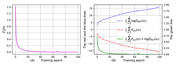
We train MLP1 designed in Section 5 on the MNIST dataset and visualize the variations of 1ni=1nlogZMLP(xi)\frac{1}{n}\sum_{i=1}^{n}\text{log}Z_{\text{MLP}}(x_{i}), 1ni=1nEyyi(xi)\frac{1}{n}\sum_{i=1}^{n}E_{yy_{i}}(x_{i}), and their summation during minimizing ^𝒮(h)\hat{\mathcal{L}}^{\ell}_{\mathcal{S}}(h) in Figure 10. We can observe that 1ni=1nlogZMLP(xi)\frac{1}{n}\sum_{i=1}^{n}\text{log}Z_{\text{MLP}}(x_{i}) is increasing and 1ni=1nEyyi(xi)\frac{1}{n}\sum_{i=1}^{n}E_{yy_{i}}(x_{i}) is decreasing. Notably, their summation 1ni=1nEyyi(xi)+logZMLP(xi)\frac{1}{n}\sum_{i=1}^{n}E_{yy_{i}}(x_{i})+\text{log}Z_{\text{MLP}}(x_{i}) has the same decreasing trend as 1ni=1nEyyi(xi)\frac{1}{n}\sum_{i=1}^{n}E_{yy_{i}}(x_{i}) and quickly converges to zero, which indicates

QFY|X(yi|xi)=1ZMLP(xi)exp[Eyyi(xi)]1.Q_{F_{Y}|X}(y_{i}|x_{i})=\frac{1}{Z_{\text{MLP}}(x_{i})}\text{exp}[-E_{yy_{i}}(x_{i})]\rightarrow 1. (65)

Recall that ZMLP(xi)=l=1Lk=1Kt=1TQ(FY,F2,F1|X=xi)Z_{\text{MLP}}(x_{i})=\sum_{l=1}^{L}\sum_{k=1}^{K}\sum_{t=1}^{T}Q(F_{Y},F_{2},F_{1}|X=x_{i}) sums up all the cases of FYF_{Y}. As a result, ZMLP(xi)Z_{\text{MLP}}(x_{i}) is a constant with respect to Q(FY|X)Q(F_{Y}|X). In other words, the functionality of ZMLP(xi)Z_{\text{MLP}}(x_{i}) is only to guarantee the validity of Q(FY|X)Q(F_{Y}|X), thus it can be viewed as a constant for deriving the generalization bound.

As a result, the PAC-Bayesian generalization bound (Equation 22) can be relaxed as

the PAC-Bayesian generalization bound1ni=1nEyyi(xi).\text{the PAC-Bayesian generalization bound}\propto\frac{1}{n}\sum_{i=1}^{n}E_{yy_{i}}(x_{i}). (66)
Refer to caption
Figure 10: (A) shows the variation of ^𝒮(h)\hat{\mathcal{L}}^{\ell}_{\mathcal{S}}(h) during 100 training epochs. (B) shows the variations of 1ni=1nlogZMLP(xi)\frac{1}{n}\sum_{i=1}^{n}\text{log}Z_{\text{MLP}}(x_{i}), 1ni=1nEyyi(xi)\frac{1}{n}\sum_{i=1}^{n}E_{yy_{i}}(x_{i}), and their summation during 100 training epochs.

G Experiments on MLPs with the Fashion-MNIST dataset

This appendix validates the PAC-Bayesian generalization bound for MLPs on the Fashion-MNIST dataset [37].

The bound can reflect the generalization of MLPs with different number of neurons.

We train the MLP={x;f1;f2;fY}\text{MLP}=\{{x;f_{1};f_{2};f_{Y}}\} with different number of neurons on the Fashion-MNIST dataset, and visualize the testing error and the bound in Figure 11. We can observe that the MLP achieves lower testing error as the number of neurons increases, and the variation of the bound is consistent with that of testing error.

Refer to caption
Figure 11: (A) and (B) show the testing error and the bound with different number of neurons, respectively.

The bound can reflect the effect of SGD optimization on the generalization of MLPs.

We specify the MLP={x;f1;f2;fY}\text{MLP}=\{{x;f_{1};f_{2};f_{Y}}\} to classify the Fashion-MNIST dataset. The MLP has 512 neurons in f1f_{1} and 256 neurons in f2f_{2}. All the activation functions are ReLU σ(z):=max(0,z)\sigma(z):=\text{max}(0,z). Since the dimension of a single Fashion-MNIST image is 28×2828\times 28, xx has M=784M=784 input nodes. Since the Fashion-MNIST dataset consists of 1010 different labels, fY{f_{Y}} has L=10L=10 output nodes. We still use three different training algorithms (the basic SGD, Momentum, and Adam) to train the MLP 200 epochs, and visualize the training error, the testing error, and the generalization bound in Figure 12.

We can observe that the bounds of the MLP with different training algorithms is consistent with the corresponding testing errors of the MLP. In contrast to Adam achieving the lowest testing error for classifying the MNIST dataset (Figure 3), Momentum achieves the lowest testing error for classifying the Fashion-MNIST dataset. Figure 12 shows the bound of the MLP with Momentum is also smaller than Adam and the basic SGD.

Refer to caption
Figure 12: (A), (B), and (C) show the training error, the testing error, and the proposed PAC-Bayesian generalization bound over 200 training epochs, respectively.

The bound can reflect the same sample size dependence as the testing error.

Similar to the experiment in Section 5, we also create 13 different subsets of the Fashion-MNIST dataset with different number of training samples, and train the MLP2 designed in Section 5 on the 13 subsets. Figure 13 shows the testing error and the bound with different sample sizes. Similar to Figure 4, the bound shows a general decreasing trend as the training sample size increases, which is consistent with the variation of the testing error.

Refer to caption
Figure 13: (A) and (B) show the testing error and the proposed PAC-Bayesian generalization bound given different training sample sizes, respectively.

The bounds can reflect the generalization performance of MLPs given random labels.

We train the MLP3 designed in Section 5 100 epochs to classify 10,000 samples of the Fashion-MNIST dataset with random labels, and visualize the training error, the testing error and the bound in Figure 14.

We observe that the bound of MLP3 trained by random labels is higher than real labels, which is consistent with the testing error based on random labels is higher than real labels.

Refer to caption
Figure 14: (A) and (B) show the testing error and the proposed PAC-Bayesian generalization bound given real labels and random labels, respectively.