PACIA: Parameter-Efficient Adapter for Few-Shot Molecular Property Prediction
Abstract
Molecular property prediction (MPP) plays a crucial role in biomedical applications, but it often encounters challenges due to a scarcity of labeled data. Existing works commonly adopt gradient-based strategy to update a large amount of parameters for task-level adaptation. However, the increase of adaptive parameters can lead to overfitting and poor performance. Observing that graph neural network (GNN) performs well as both encoder and predictor, we propose PACIA, a parameter-efficient GNN adapter for few-shot MPP. We design a unified adapter to generate a few adaptive parameters to modulate the message passing process of GNN. We then adopt a hierarchical adaptation mechanism to adapt the encoder at task-level and the predictor at query-level by the unified GNN adapter. Extensive results show that PACIA obtains the state-of-the-art performance in few-shot MPP problems, and our proposed hierarchical adaptation mechanism is rational and effective.
1 Introduction
Molecular property prediction (MPP) which predicts whether desired properties will be active on given molecules, can be naturally modeled as a few-shot learning problem Waring et al. (2015); Altae-Tran et al. (2017). As wet-lab experiments to evaluate the actual properties of molecules are expensive and risky, usually only a few labeled molecules are available for a specific property. While recently, Graph Neural Network (GNN) is popularly used to learn molecular representations Xu et al. (2019); Yang et al. (2019); Xiong et al. (2019). Modeling molecules as graphs, GNN can capture inherent structural information. Hence, GNN-based methods obtain better performance than classical ones Unterthiner et al. (2014); Ma et al. (2015), especially when they are pretrained on self-learning tasks constructed from additional large scale corpus. As for tasks with only a few labeled molecules, the performance of existing GNN-based methods is still far from desired.
Various few-shot learning (FSL) methods have been developed to handle few-shot MPP problem. The earlier work IterRefLSTM Altae-Tran et al. (2017) builds a metric-based model upon matching network Vinyals et al. (2016). Subsequent works mainly adopt gradient-based meta-learning strategy Finn et al. (2017), which learns parameter initialization with good generalizability across different properties and adapts parameters by gradient descent for target property. Specifically, Meta-MGNN Guo et al. (2021) brings chemical prior knowledge in the form of molecular reconstruction loss, and optimizes all parameters by gradient descents. PAR Wang et al. (2021) introduces attention and relation graph module to better utilize the labeled samples for property-adaptation with the awareness of target chemical property, and conducts a selective gradient-based meta-learning strategy. ADKF-IFT Chen et al. (2022) takes a gradient-based meta-learning strategy with implicit function theorem to avoid computing expensive hypergradients, and builds a Gaussian Process for each task as classifier. There are also works that bring auxiliary information such as additional reference molecules from large molecule database Schimunek et al. (2023) and auxiliary properties Zhuang et al. (2023) to improve the performance of few-shot MPP Schimunek et al. (2023); Zhuang et al. (2023).
Two primary issues persist in existing studies. First, gradient-based meta-learning strategy requires updating a large number of parameters in order to adapt to each task. This results in poor learning efficiency and is prone to overfit given insufficient labeled samples Rajeswaran et al. (2019); Yin et al. (2020), as demonstrated in Figure 1 (a). While with more task-specific parameters, the model gets easily overfit, which would be more severe in extreme few-shot cases. Effective adaptation should be made in a parameter-efficient way, i.e, without modulating a large amount of parameters. Second, query-level adaptation is absent but it is important specially for few-shot MPP. The chemical space is enormous and the representations of molecules vary in a wide range. The query-level difference should be addressed when classifying the encoded molecules. When query molecules are more similar to the labeled molecules in one class, they can be easily classified. While others exhibit comparable similarity to both categories, they will be harder to be accurately classified. Thus, a fixed predictor can not fit all molecules even in a single task.
In this paper, we first summarize existing works into an encoder-predictor framework, where GNN performs well acting as both encoder and predictor. Upon the framework, we propose PACIA, a PArameter-effiCIent Adapter for few-shot MPP problem. To sum up, our contributions are as follows:
-
•
We propose query-level adaptation for few-shot MPP problem and design a hierarchical adaptation mechanism for the encoder-predictor framework generally adopted by existing approaches.
-
•
We design a hypernetwork-based GNN adapter to achieve parameter-efficient adaptation. This unified GNN adapter can generate a few adaptive parameters to modulate the message passing process of GNN in two aspects: node embedding and propagation depth.
- •
2 Related Works
2.1 Few-Shot Learning
Few-shot learning (FSL) aims to generalize to a task with a few labeled samples Wang et al. (2020). In terms of adaptation mechanism, existing FSL methods can be classified into three main categories: (i) gradient-based approaches Finn et al. (2017); Grant et al. (2018) learn a model which can be generalized to new task by gradient descents, (ii) metric-based approaches Vinyals et al. (2016); Snell et al. (2017) learn to embed samples into a space where similar and dissimilar samples can be easily discriminated by a distance function, and (iii) amortization-based approaches Requeima et al. (2019); Lin et al. (2021); Przewiezlikowski et al. (2022) use hypernetworks to map the labeled samples in the task to a few parameters to adjust the main networks to be task-specific. Recent works Requeima et al. (2019) found that amortization-based approaches can reduce the risk of overfitting compared with gradient-based approaches. They also have faster inference speed as the adapted parameters are generated by a single forward pass without taking optimization steps. Besides, the main networks can approximate various functions in addition to distance-based ones.
2.2 Hypernetworks
Hypernetworks Ha et al. (2017) refer to neural networks which learn to generate parameters of the main network which handles the target tasks. Hypernetworks have been successfully used in various applications like cold-start recommendation Lin et al. (2021) and image classification Przewiezlikowski et al. (2022). Designing appropriate hypernetworks is challenging, requiring domain knowledge to decide what information to be fed into hypernetworks, how to adapt the main network, and what is the appropriate architecture of hypernetworks. For general GNNs, hypernetworks are developed to modulate weight matrix in aggregation function in message passing Brockschmidt (2020), or to facilitate node-specific message passing Nachmani and Wolf (2020). In contrast to them, we particularly consider designing parameter-efficient modulators for GNNs used in encoder-predictor framework for few-shot MPP.
3 Preliminaries: Few-Shot MPP
3.1 Problem Setup
In a few-shot MPP task with respect to a specific property, each sample is a molecular graph and its label records whether the molecule is active or inactive on the target property. Only a few labeled samples are available in . Following earlier works Altae-Tran et al. (2017); Stanley et al. (2021); Chen et al. (2022); Schimunek et al. (2023), we model a as a -way classification task , associating with a support set containing labeled samples from active/inactive class, and a query set containing samples whose labels are only used for evaluation. We consider both (i) balanced support sets, i.e., contains samples per class which is consistent with the standard -way -shot FSL setting Altae-Tran et al. (2017), and (ii) imbalanced support sets which exist in real-world applications Stanley et al. (2021). Our target is to learn a model from a set of tasks that can generalize to new task given the few-shot support set. Specifically, the target properties are different across tasks.
3.2 Encoder-Predictor Framework
In the past, molecules are encoded with certain properties (fingerprint vectors Rogers and Hahn (2010)) and fed to deep networks for prediction Unterthiner et al. (2014); Ma et al. (2015). While recently, GNNs are popularly taken as molecular encoders Li et al. (2018); Yang et al. (2019); Xiong et al. (2019); Hu et al. (2019) due to their superior performance on learning from of topological data. In either case, existing works can be summarized within an encoder-predictor framework.
Consider a molecular graph with node feature for each atom and edge feature for each chemical bond between atoms . A GNN encoder maps to molecular representation which is a fixed-length vector. At the th layer, GNN updates atom embedding of as
| (1) |
where contains neighbors of . AGG() and UPD() are aggregation and updating functions respectively. After layers, the query-level representation for is obtained as
| (2) |
where function aggregates atom embeddings.
Then, a predictor assigns label for a query molecule given support molecules in :
| (3) |
The specific choice of is diverse, e.g., pair-wise similarity Altae-Tran et al. (2017), multi-layer perceptron (MLP) Guo et al. (2021); Wang et al. (2021) and Mahalanobis distance Stanley et al. (2021). Recently, GNN-based predictor which operates on relation graphs of molecules is found to effectively compensate for the lack of supervised information Wang et al. (2021). In particular, molecular representations are refined on relation graphs such that the similar molecules cluster closer. Initialize molecular representations as the output of the encoder, i.e., . Denote the set of molecules as , which contains all information to make prediction for the query molecule . The relation graph works by recurrently estimating the adjacency matrix and updating the molecular representations. At the th layer, each element in the adjacent matrix of the relation graph is learned to represent pair-wise similarities between any two molecules in :
| (4) |
Then, each molecular representation is refined as
| (5) |
After layers of refinement, and (in place of and ) are fed to (3) to obtain final prediction for .
4 Hierarchical Adaptation of Encoder-Predictor Framework
To generalize across different tasks with a few labeled molecules, existing works Wang et al. (2021); Chen et al. (2022) usually conduct task-level adaptation by gradient-based meta-learning. (see Appendix A). However, as discussed in Section 2, gradient-based meta-learning optimizes most parameters using a few labeled molecules, which is slow to optimize and easy to overfit. As for query-level adaptation, gradient is not accessible for each query molecule in testing since the label is unknown during training. Therefore, we turn to hypernetworks to achieve parameter-efficient adaptation. Task-level adaptation is achieved in encoder since the structural features in molecular graphs needs to be captured in a property-adaptive manner, while query-level adaptation is achieved in predictor based on the property-adaptive representations.
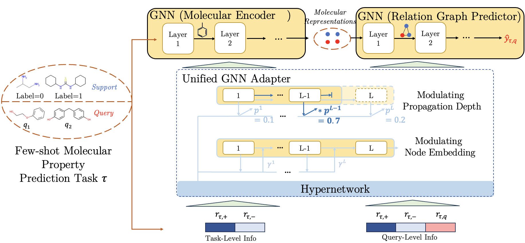
As discussed in Section 3.2, GNNs can effectively act as both encoder and predictor. Therefore, we propose PACIA (Figure 1), a method using a unified GNN adapter to generate a few adaptive parameters to hierarchically adapt the encoder at task-level and the predictor at query-level in a parameter-efficient manner. In the sequel, we provide the details of the unified GNN adapter (Section 4.1), then describe how to learn the main networks (including encoder and predictor) with the unified GNN adapter by episodic training (Section 4.2). Finally, we present a comparative discussion of PACIA in relation to existing works (Section 4.3).
4.1 A Unified GNN Adapter
To adapt GNN’s parameter-efficiently, we design a GNN adapter to modulate the node embedding and propagation depth, which are essential in message passing process.
Modulating Node Embedding.
Denote the node embedding at the th layer as , which can be atom embedding in encoder or molecular embedding in relation graph predictor. We obtain adapted embedding as
| (6) |
where is an element-wise function, and is adaptive parameter generated by the hypernetworks. This adapted embedding is then fed to next layer of GNN.
Modulating Propagation Depth.
Further, we manage to modulate the propagation depth, i.e., layer number of a GNN. Controlling is challenging since it is discrete. We achieve this by training a differentiable controller, which is a hypernetwork to generate a scalar corresponding to the th layer. The value of estimates how likely the message passing should stop after the th layer. Finally, assume there are layers in total, the vector
| (7) |
represents the plausibility of choosing each layer. The hypernetwork is shared across all layers. During meta-training, is used as differentiable weight to modulate GNN layers. Specifically, after propagation through all layers, the final node embedding is obtained as
| (8) |
where is the th element of .
Generating Adaptive Parameters.
We generate adaptive parameters by hypernetworks. In particular, note that the generated adaptive parameter should be permutation-invariant to the order of input samples in . Therefore, we first calculate class prototypes and of active class (+) and inactive class (-) for samples in by
| (9) | ||||
where means concatenating, and are the sets of active and inactive samples in , and is the one-hot encoding of label. Using and allows subsequent steps to keep supervised information while being permutation-invariant.
Recall that task-level adaptation and query-level adaptation is achieved in encoder and predictor respectively. For task-level adaptation, we then map and to as
| (10) |
As for query-level adaptation, information comes from both and the specific query molecule . Likewise, we use class prototypes and to keep permutation-invariant. We then generate as
| (11) |
combining information in and . Note that parameters of these MLPs in hypernetworks are jointly meta-learned with the encoder and predictor.
4.2 Learning and Inference
Denote the collection of all model parameters in main network((1)-(5)) and hypernetwork ((9)-(11)) as , excluding adaptive parameters. Our objective takes the form:
| (12) |
is the loss in task , is one-hot ground-truth label vector and is prediction obtained by (3).
Note that is shared across all tasks. While the adaptive parameter in (6) and in (7) are generated by hypernetworks. The size of adaptive parameter is far smaller than the main network. This realizes parameter-efficient adaptation and mitigates the risk of overfitting.
Algorithm 1111In Algorithm 1 and 4,“*” (resp. “+”) indicates the step is executed by the main network (resp. hypernetwork). summarizes the training procedure of PACIA. As mentioned above, our unified GNN adapter can simultaneously modulate the node embedding and propagation depth, and be cascaded to adapt both encoder and predictor. During training, molecular graph is first processed by encoder (line 4-9). At each layer, adaptive parameters are obtained by (10) (line 5). Then, (6) modulates all atom embeddings (line 6). After layers of message passing (1), (8) is applied before (2), to get property-adaptive molecular representations and initialize node embeddings in relation graph (line 9). Then in predictor, at each layer of GNN on relation graph, adaptive parameters are obtained with (11) (line 13) and (6) modulates all node embeddings (line 14). After layers of message passing by (4)(5), (8) is applied (line 17). The final prediction is obtained by (3).
Testing procedure is provided in Appendix B. The process is similar. A noteworthy difference is the propagation depth is adapted by selecting the layer with maximal plausibility:
| (13) |
Only , rather than (8), is fed forward to the next module.
| Method | Tox21 | SIDER | MUV | ToxCast | ||||
|---|---|---|---|---|---|---|---|---|
| 10-shot | 1-shot | 10-shot | 1-shot | 10-shot | 1-shot | 10-shot | 1-shot | |
| GNN-ST | ||||||||
| MAT | ||||||||
| GNN-MT | ||||||||
| ProtoNet | ||||||||
| MAML | ||||||||
| Siamese | - | - | ||||||
| EGNN | ||||||||
| IterRefLSTM | - | - | ||||||
| PAR | ||||||||
| ADKF-IFT | ||||||||
| PACIA | ||||||||
4.3 Comparison with Existing Works
From the perspective of hypernetworks, the usage of hypernetworks for encoder is related to GNN-FiLM Brockschmidt (2020), which considers a GNN as main network. It builds hypernetworks with target node as input to generate parameters of FiLM layers, to equip different nodes with different aggregation functions in the GNN. What and how to adapt are similar to ours, but it is different that the input of our hypernetworks for encoder is and how we encode a set of labeled graphs.
As for few-shot learning, some recent studies Requeima et al. (2019); Lin et al. (2021) use hypernetworks to transform the support set into parameters that modulate the main network. The functionality of their hypernetworks is akin to that of our hypernetwork for the encoder. However, there is a distinct difference in the architecture of main networks: while their approaches employ convolutional neural networks and MLPs, our method uniquely modulates the message passing process of GNN. Furthermore, the application of hypernetworks for the predictor, aimed at adjusting the model architecture based on a query sample (without label information) and a set of labeled samples, has not yet been explored in the literature. A detailed comparison of PACIA w.r.t. existing few-shot MPP works is in Appendix C.
5 Experiments
In this section, we evaluate the proposed PACIA222Code is available at https://github.com/LARS-research/PACIA. on few-shot MPP problems. We run all experiments with 10 random seeds, and report the mean and standard deviations (in the subscript bracket). Appendix D provides more information of datasets, baselines, and implementation details.
5.1 Performance Comparison on MoleculeNet
We use Tox21 National Center for Advancing Translational Sciences (2017), SIDER Kuhn et al. (2016), MUV Rohrer and Baumann (2009) and ToxCast Richard et al. (2016) from MoleculeNet Wu et al. (2018), which are commonly used to evaluate the performance on few-shot MPP Altae-Tran et al. (2017); Wang et al. (2021). We adopt the public data split provided by Wang et al. (2021). The support sets are balanced, each of them contains labeled molecules per class, where and are considered. The performance is evaluated by ROC-AUC calculated on the query set of each meta-testing task and averaged across all meta-testing tasks.
We compare PACIA with the following baselines: 1) single-task method GNN-ST Gilmer et al. (2017); 2) multi-task pretraining method GNN-MT Corso et al. (2020); Gilmer et al. (2017); 3) self-supervised pretraining method MAT Maziarka et al. (2020); 4) meta-learning methods, including Siamese Koch et al. (2015), ProtoNet Snell et al. (2017), MAML Finn et al. (2017), EGNN Kim et al. (2019); and 5) methods proposed for few-shot MPP, including IterRefLSTM Altae-Tran et al. (2017), PAR Wang et al. (2021) and ADKF-IFT Chen et al. (2022). Note that MHNfs Schimunek et al. (2023) is not included as it uses additional reference molecules from external datasets, which leads to unfair comparison. GS-META Zhuang et al. (2023) has not been compared since that approach requires multiple properties of each molecule, which is not applicable when a molecule is only evaluated w.r.t. one property. Following earlier works Guo et al. (2021); Wang et al. (2021), we use GIN Xu et al. (2019) as encoder, which is trained from scratch.
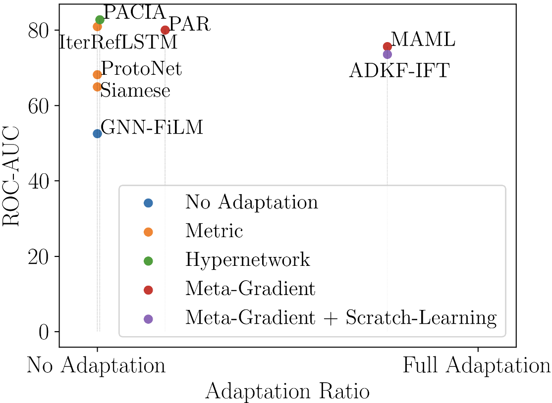
Table 1 shows the results. Results of Siamese and IterRefLSTM are copied from Altae-Tran et al. (2017) as their codes are unavailable, and their results on ToxCast are unknown. GNN-FiLM is a general GNN whose target is not few-shot MPP, which explains its bad performance. PACIA obtains the highest ROC-AUC scores on all cases except the 10-shot case on MUV, where ADKF-IFT outperforms the others by a large margin. This can be a special case where ADKF-IFT works well but may not be generalizable. Moreover, depending on the number of local-update steps of ADKF-IFT, PACIA is about 5 times faster than ADKF-IFT (both meta-training and inference time is about 1/5). In terms of average performance, PACIA significantly outperforms the second-best method ADKF-IFT by 3.25%. We also provide results obtained with a pretrained encoder in Appendix D.3. Similar observations can be made: our PACIA with pretrained encoder (Pre-PACIA) performs the best, and its performance gain is more significant when fewer labeled samples are provided. Further, results in Appendix D.4 shows the performance comparison between PACIA and a fine-tuned GNN with varying support set size. This shows that PACIA nicely achieves its goal: handling few-shot MPP problem in a parameter-efficient way.
5.2 Performance Comparison on FS-Mol
We also use FS-Mol Stanley et al. (2021), a new benchmark consisting of a large number of diverse tasks for model pretraining and a set of few-shot tasks with imbalanced classes. We adopt the public data split Stanley et al. (2021). Each support set contains 64 labeled molecules, and can be imbalanced where the number of labeled molecules from active and inactive is not equal. All remaining molecules in the task form the query set. Testing tasks are divided into categories with support size 16 Schimunek et al. (2023), which is close to real-world scenario. The performance is evaluated by AUPRC (change in area under the precision-recall curve) w.r.t. a random classifier Stanley et al. (2021), averaged across meta-testing tasks.
We use the same baselines that were applied to MoleculeNet. Table 2 shows the results. We find that PACIA performs the best. Besides, the time-efficiency of PACIA is much higher since its adaptation only needs a single forward pass. While IterRefLSTM and ADKF-IFT take multiple local-update steps, they are much slower to generalize.
| Method | All | Kinases | Hydrolases | Oxido- |
|---|---|---|---|---|
| [157] | [125] | [20] | reductases[7] | |
| GNN-ST | ||||
| MAT | ||||
| GNN-MT | ||||
| MAML | ||||
| PAR | ||||
| ProtoNet | ||||
| EGNN | ||||
| Siamese | ||||
| IterRefLSTM | ||||
| ADKF-IFT | ||||
| PACIA |
5.3 Ablation Study
We consider various variants of PACIA, including (i) fine-tuning: using the same model structure and fine-tuning all parameters to adapt to each property without hypernetworks; (ii) w/o T: removing task-level adaptation, thus the GNN encoder will not be adapted by hypernetworks w.r.t. each property; and (iii) w/o Q: removing query-level adaptation, such that all molecules are processed by the same predictor.
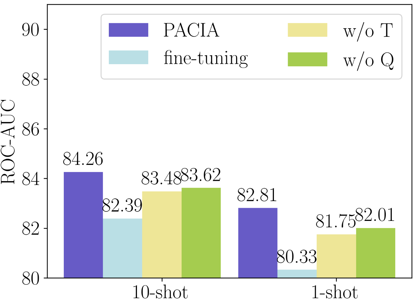
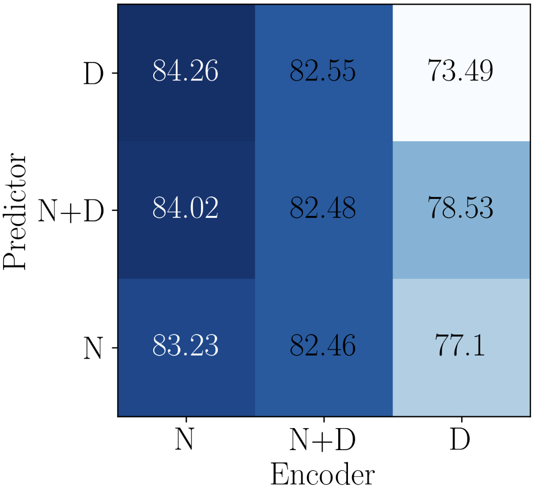
Figure 2(a) provides performance comparison on Tox21. As shown, the performance gain of PACIA over “w/o Q” shows the necessity of query-level adaptation. The gap between PACIA and “w/o T” indicates the effect of adapting the model to be task-specific. One can also notice that without query-level adaptation, “w/o Q” still obtains better performance than gradient-based baselines like PAR, which indicates the advantage of designing the amortization-based hypernetwork. The poor performance of “fine-tuning” is possibly because of the overfitting caused by updating all parameters with only a few samples. In sum, every component of PACIA is important for achieving good performance.
Now that the effectiveness of task-level and query-level adaptation are validated, we further investigate modulation functions, i.e, modulating node embedding (N), modulating propagation depth (D), modulating both (ND), for encoder and predictor. There are combinations, whose performance is reported in Figure 2(b). We find that only modulating node embedding in encoder while only modulating propagation depth in predictor obtains the best performance. As the GIN encoder has highly non-linearity across layers, truncation would lead to non-explainability and somehow perturb the black-box. While the operation of relation graph in predictor updates node embedding in a linear way (5), adapting the propagation depth is harmonious with message passing process.
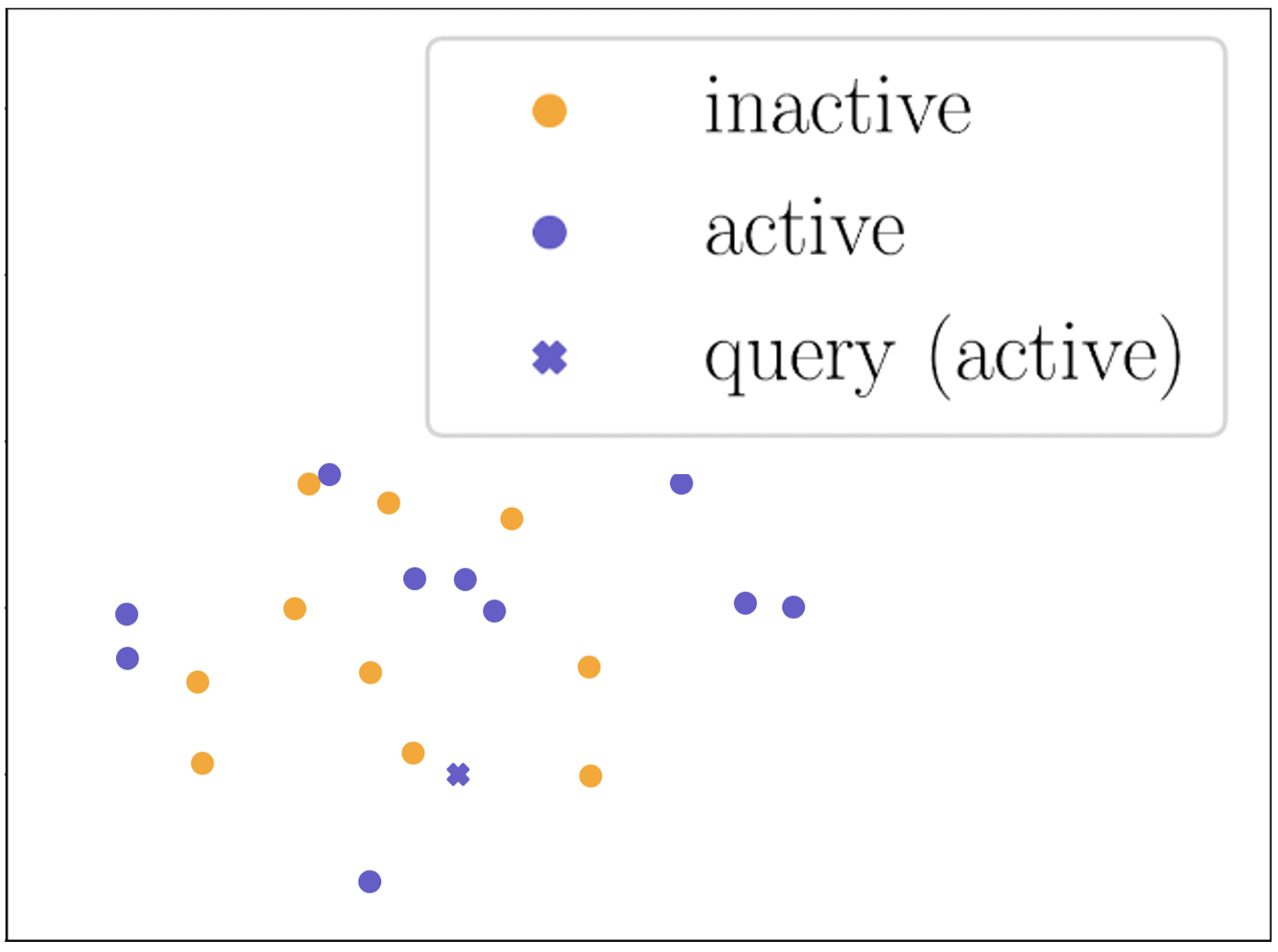
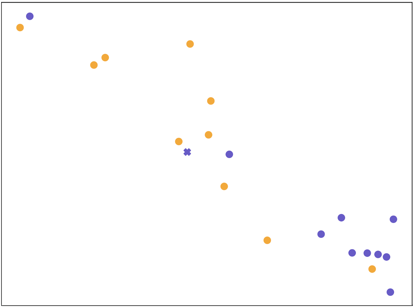
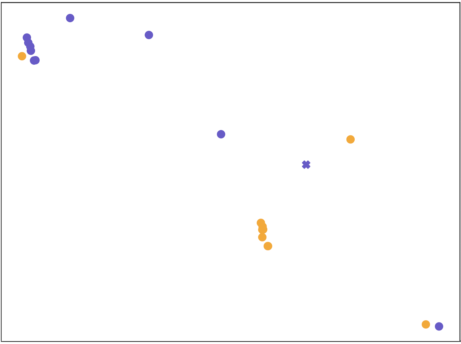
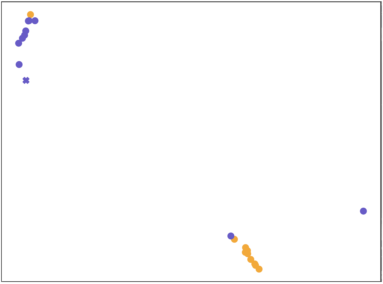
Figure 3 shows the t-SNE visualization Van der Maaten and Hinton (2008) of molecular representations learned on a 10-shot support set and a query molecule with ground-truth label “active” in task SR-p53 from Tox21. As shown, molecular representations obtained without adaptation (Figure 3(a)) are mixed up, since the encoder has not been adapted to the target property of the task. Molecular representations being processed by our property-adaptive encoder (Figure 3(b)) becomes more distinguishable, indicating that adapting molecular representation in task-level takes effect. Molecular representations in Figure 3(c) and Figure 3(d) form clear clusters as we encourage similar molecules to be connected during relation graph refinement by (5). The difference is that molecular representations in Figure 3(c) are refined by the best propagation depth number for all tasks in 10-shot case, while molecular representations in Figure 3(d) are refined by 4 depths of propagation which are selected for the specific query molecule. As shown, we can conclude that our molecular-adaptive refinement steps help better separate molecules of different classes. Ablation study of configurations of hypernetworks is in Appendix D.5.
5.4 Study of Hierarchical Adaptation Mechanism
Task-Level Adaptation.
In PACIA, parameter-efficient task-level adaptation is achieved by using hypernetworks to modulate the node embeddings during message passing. We compared this amortization-based adaptation with gradient-based adaptation in PAR which has similar main network with PACIA. We record their adaptation process, i.e., time required to process the support set and the test performance. Table 3 shows the results. PAR uses molecules in support set to take gradient steps, and updates all parameters in GNN. We record each of a maximum five steps, where we can find that it easily overfits as the testing ROC-AUC keeps dropping with more steps. The time consumption also grows. In contrast, PACIA processes molecules in support set by hypernetworks, which is much more efficient as only one single forward pass is needed. PACIA can obtain better performance due to the reduction of adaptive parameters, which also leads to better generalization and alleviates the risk of overfitting to a few shots. Table 3 and Figure 1(a) both indicate that the underlying overfitting problem can be mitigated by PACIA.
| PACIA | PAR | |||||
|---|---|---|---|---|---|---|
| # Total para. | 3.28M | 2.31M | ||||
| # Adaptive para. | 3.00K | 0.38M | ||||
| # Gradient steps | - | 1 | 2 | 3 | 4 | 5 |
| ROC-AUC (%) | 84.26 | 82.07 | 81.85 | 80.32 | 79.09 | 77.25 |
| Time (secs) | 1.09 | 2.02 | 3.62 | 5.34 | 6.76 | 8.10 |
Query-Level Adaptation.
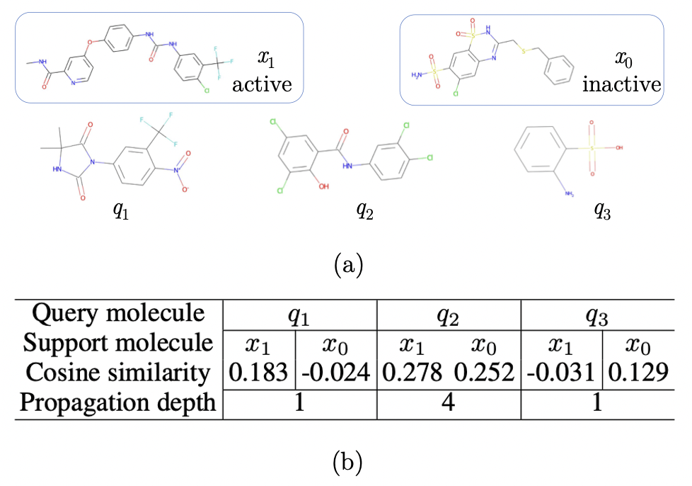
Finally, we present a case study on query-level adaptation. More experimental results on validating the design of query-level adaptation are in Appendix D.6. We use a 1-shot support set and 3 query molecules in task SR-p53 of Tox21. In Figure 4(a), and are support molecules with different labels, , and are query molecules. As shown, classifying and is relatively easy and the propagation depth will be 1, while classifying is hard and requires 4 depth of propagation. Considering the shared substructures (function groups), and are visually similar, and are visually similar. While both and share substructures with , it is hard to tell which of them is more similar to . Figure 4(a) provides the cosine similarity based on the molecule representations generated by Pre-GNN , which confirms our observation: is much more similar to , is much more similar to , and shows large similarities with both samples. Intuitively, classifying and will be easier while will be hard. In the dynamic propagation of PACIA, we find different depths are taken: 1 for both and while 4 for . PACIA achieves effective query-level adaptation by assigning more complex models for query molecules that are difficult to classify.
6 Conclusion
We propose PACIA to handle few-shot MPP in a parameter-efficient manner. We investigate two key factors in few-shot molecular property prediction under the common encoder-predictor framework: adaptation-efficiency and query-level adaptation. Evidence shows that too much adaptive parameter would lead to overfitting, thus we design a parameter-efficient GNN adapter, which can modulate node embedding and propagation depth of message passing of GNN in a unified way. We also notice the importance of capturing query-level difference and therefore propose hierarchical adaptation mechanism, which is achieved by using a unified GNN adapter in both encoder and predictor. Empirical results show that PACIA achieves the best performance on both MoleculeNet and FS-Mol.
Acknowledgments
Q. Yao is supported by research fund of National Natural Science Foundation of China (No. 92270106), and Independent Research Plan of the Department of Electronic Engineering Department at Tsinghua University.
References
- Altae-Tran et al. [2017] Han Altae-Tran, Bharath Ramsundar, Aneesh S Pappu, and Vijay Pande. Low data drug discovery with one-shot learning. ACS Central Science, 3(4):283–293, 2017.
- Brockschmidt [2020] Marc Brockschmidt. GNN-FiLM: Graph neural networks with feature-wise linear modulation. In International Conference on Machine Learning, pages 1144–1152, 2020.
- Chen et al. [2022] Wenlin Chen, Austin Tripp, and José Miguel Hernández-Lobato. Meta-learning adaptive deep kernel gaussian processes for molecular property prediction. In International Conference on Learning Representations, 2022.
- Corso et al. [2020] Gabriele Corso, Luca Cavalleri, Dominique Beaini, Pietro Liò, and Petar Veličković. Principal neighbourhood aggregation for graph nets. In Advances in Neural Information Processing Systems, pages 13260–13271, 2020.
- Finn et al. [2017] Chelsea Finn, Pieter Abbeel, and Sergey Levine. Model-agnostic meta-learning for fast adaptation of deep networks. In International Conference on Machine Learning, pages 1126–1135, 2017.
- Gilmer et al. [2017] Justin Gilmer, Samuel S Schoenholz, Patrick F Riley, Oriol Vinyals, and George E Dahl. Neural message passing for quantum chemistry. In International Conference on Machine Learning, pages 1263–1272, 2017.
- Grant et al. [2018] Erin Grant, Chelsea Finn, Sergey Levine, Trevor Darrell, and Thomas Griffiths. Recasting gradient-based meta-learning as hierarchical Bayes. In International Conference on Learning Representations, 2018.
- Guo et al. [2021] Zhichun Guo, Chuxu Zhang, Wenhao Yu, John Herr, Olaf Wiest, Meng Jiang, and Nitesh V Chawla. Few-shot graph learning for molecular property prediction. In The Web Conference, pages 2559–2567, 2021.
- Ha et al. [2017] David Ha, Andrew Dai, and Quoc V Le. Hypernetworks. In International Conference on Learning Representations, 2017.
- Hou et al. [2022] Zhenyu Hou, Xiao Liu, Yuxiao Dong, Chunjie Wang, Jie Tang, et al. GraphMAE: Self-supervised masked graph autoencoders. In ACM SIGKDD International Conference on Knowledge Discovery & Data Mining, pages 594–604, 2022.
- Hu et al. [2019] Weihua Hu, Bowen Liu, Joseph Gomes, Marinka Zitnik, Percy Liang, Vijay Pande, and Jure Leskovec. Strategies for pre-training graph neural networks. In International Conference on Learning Representations, 2019.
- Kim et al. [2019] Jongmin Kim, Taesup Kim, Sungwoong Kim, and Chang D Yoo. Edge-labeling graph neural network for few-shot learning. In IEEE/CVF Conference on Computer Vision and Pattern Recognition, pages 11–20, 2019.
- Koch et al. [2015] Gregory Koch, Richard Zemel, and Ruslan Salakhutdinov. Siamese neural networks for one-shot image recognition. In ICML Deep Learning Workshop, 2015.
- Kuhn et al. [2016] Michael Kuhn, Ivica Letunic, Lars Juhl Jensen, and Peer Bork. The SIDER database of drugs and side effects. Nucleic Acids Research, 44(D1):D1075–D1079, 2016.
- Li et al. [2018] Ruoyu Li, Sheng Wang, Feiyun Zhu, and Junzhou Huang. Adaptive graph convolutional neural networks. In AAAI Conference on Artificial Intelligence, pages 3546–3553, 2018.
- Lin et al. [2021] Xixun Lin, Jia Wu, Chuan Zhou, Shirui Pan, Yanan Cao, and Bin Wang. Task-adaptive neural process for user cold-start recommendation. In The Web Conference, pages 1306–1316, 2021.
- Ma et al. [2015] Junshui Ma, Robert P Sheridan, Andy Liaw, George E Dahl, and Vladimir Svetnik. Deep neural nets as a method for quantitative structure–activity relationships. Journal of Chemical Information and Modeling, 55(2):263–274, 2015.
- Maziarka et al. [2020] Lukasz Maziarka, Tomasz Danel, Slawomir Mucha, Krzysztof Rataj, Jacek Tabor, and Stanislaw Jastrzebski. Molecule attention transformer. arXiv preprint arXiv:2002.08264, 2020.
- Mendez et al. [2019] David Mendez, Anna Gaulton, A Patrícia Bento, Jon Chambers, Marleen De Veij, Eloy Félix, María Paula Magariños, Juan F Mosquera, Prudence Mutowo, Michał Nowotka, et al. Chembl: towards direct deposition of bioassay data. Nucleic Acids Research, 47(D1):D930–D940, 2019.
- Nachmani and Wolf [2020] Eliya Nachmani and Lior Wolf. Molecule property prediction and classification with graph hypernetworks. arXiv preprint arXiv:2002.00240, 2020.
- National Center for Advancing Translational Sciences [2017] National Center for Advancing Translational Sciences. Tox21 challenge. http://tripod.nih.gov/tox21/challenge/, 2017. Accessed: 2016-11-06.
- Perez et al. [2018] Ethan Perez, Florian Strub, Harm De Vries, Vincent Dumoulin, and Aaron Courville. FiLM: Visual reasoning with a general conditioning layer. In AAAI Conference on Artificial Intelligence, pages 3942–3951, 2018.
- Przewiezlikowski et al. [2022] Marcin Przewiezlikowski, P Przybysz, Jacek Tabor, Maciej Zieba, and Przemyslaw Spurek. HyperMAML: Few-shot adaptation of deep models with hypernetworks. arXiv preprint arXiv:2205.15745, 2022.
- Rajeswaran et al. [2019] Aravind Rajeswaran, Chelsea Finn, Sham M Kakade, and Sergey Levine. Meta-learning with implicit gradients. In Advances in Neural Information Processing Systems, pages 113–124, 2019.
- Requeima et al. [2019] James Requeima, Jonathan Gordon, John Bronskill, Sebastian Nowozin, and Richard E Turner. Fast and flexible multi-task classification using conditional neural adaptive processes. In Advances in Neural Information Processing Systems, pages 7957–7968, 2019.
- Richard et al. [2016] Ann M Richard, Richard S Judson, Keith A Houck, Christopher M Grulke, Patra Volarath, Inthirany Thillainadarajah, Chihae Yang, James Rathman, Matthew T Martin, John F Wambaugh, et al. ToxCast chemical landscape: Paving the road to 21st century toxicology. Chemical Research in Toxicology, 29(8):1225–1251, 2016.
- Rogers and Hahn [2010] David Rogers and Mathew Hahn. Extended-connectivity fingerprints. Journal of Chemical Information and Modeling, 50(5):742–754, 2010.
- Rohrer and Baumann [2009] Sebastian G Rohrer and Knut Baumann. Maximum unbiased validation (MUV) data sets for virtual screening based on PubChem bioactivity data. Journal of Chemical Information and Modeling, 49(2):169–184, 2009.
- Schimunek et al. [2023] Johannes Schimunek, Philipp Seidl, Lukas Friedrich, Daniel Kuhn, Friedrich Rippmann, Sepp Hochreiter, and Günter Klambauer. Context-enriched molecule representations improve few-shot drug discovery. arXiv preprint arXiv:2305.09481, 2023.
- Snell et al. [2017] Jake Snell, Kevin Swersky, and Richard Zemel. Prototypical networks for few-shot learning. In Advances in Neural Information Processing Systems, pages 4080–4090, 2017.
- Stanley et al. [2021] Megan Stanley, John F Bronskill, Krzysztof Maziarz, Hubert Misztela, Jessica Lanini, Marwin Segler, Nadine Schneider, and Marc Brockschmidt. FS-Mol: A few-shot learning dataset of molecules. In Neural Information Processing Systems Track on Datasets and Benchmarks, 2021.
- Sterling and Irwin [2015] Teague Sterling and John J Irwin. ZINC 15–ligand discovery for everyone. Journal of Chemical Information and Modeling, 55(11):2324–2337, 2015.
- Unterthiner et al. [2014] Thomas Unterthiner, Andreas Mayr, Günter Klambauer, Marvin Steijaert, Jörg K Wegner, Hugo Ceulemans, and Sepp Hochreiter. Deep learning as an opportunity in virtual screening. In NIPS Deep Learning Workshop, volume 27, pages 1–9, 2014.
- Van der Maaten and Hinton [2008] Laurens Van der Maaten and Geoffrey Hinton. Visualizing data using t-SNE. Journal of Machine Learning Research, 9(11), 2008.
- Vinyals et al. [2016] Oriol Vinyals, Charles Blundell, Timothy Lillicrap, Daan Wierstra, et al. Matching networks for one shot learning. In Advances in Neural Information Processing Systems, pages 3630–3638, 2016.
- Wang et al. [2020] Yaqing Wang, Quanming Yao, James T Kwok, and Lionel M Ni. Generalizing from a few examples: A survey on few-shot learning. ACM Computing Surveys, 53(3):1–34, 2020.
- Wang et al. [2021] Yaqing Wang, Abulikemu Abuduweili, Quanming Yao, and Dejing Dou. Property-aware relation networks for few-shot molecular property prediction. In Advances in Neural Information Processing Systems, pages 17441–17454, 2021.
- Waring et al. [2015] Michael J Waring, John Arrowsmith, Andrew R Leach, Paul D Leeson, Sam Mandrell, Robert M Owen, Garry Pairaudeau, William D Pennie, Stephen D Pickett, Jibo Wang, et al. An analysis of the attrition of drug candidates from four major pharmaceutical companies. Nature Reviews Drug discovery, 14(7):475–486, 2015.
- Wu et al. [2018] Zhenqin Wu, Bharath Ramsundar, Evan N Feinberg, Joseph Gomes, Caleb Geniesse, Aneesh S Pappu, Karl Leswing, and Vijay Pande. MoleculeNet: A benchmark for molecular machine learning. Chemical Science, 9(2):513–530, 2018.
- Wu et al. [2023] Shiguang Wu, Yaqing Wang, Qinghe Jing, Daxiang Dong, Dejing Dou, and Quanming Yao. ColdNAS: Search to modulate for user cold-start recommendation. In The Web Conference, pages 1021–1031, 2023.
- Xiong et al. [2019] Zhaoping Xiong, Dingyan Wang, Xiaohong Liu, Feisheng Zhong, Xiaozhe Wan, Xutong Li, Zhaojun Li, Xiaomin Luo, Kaixian Chen, Hualiang Jiang, et al. Pushing the boundaries of molecular representation for drug discovery with the graph attention mechanism. Journal of Medicinal Chemistry, 63(16):8749–8760, 2019.
- Xu et al. [2019] Keyulu Xu, Weihua Hu, Jure Leskovec, and Stefanie Jegelka. How powerful are graph neural networks? In International Conference on Learning Representations, 2019.
- Xu et al. [2021] Minghao Xu, Hang Wang, Bingbing Ni, Hongyu Guo, and Jian Tang. Self-supervised graph-level representation learning with local and global structure. In International Conference on Machine Learning, pages 11548–11558, 2021.
- Yang et al. [2019] Kevin Yang, Kyle Swanson, Wengong Jin, Connor Coley, Philipp Eiden, Hua Gao, Angel Guzman-Perez, Timothy Hopper, Brian Kelley, Miriam Mathea, et al. Analyzing learned molecular representations for property prediction. Journal of Chemical Information and Modeling, 59(8):3370–3388, 2019.
- Yin et al. [2020] Mingzhang Yin, George Tucker, Mingyuan Zhou, Sergey Levine, and Chelsea Finn. Meta-learning without memorization. In International Conference on Learning Representations, 2020.
- Zhuang et al. [2023] Xiang Zhuang, Qiang Zhang, Bin Wu, Keyan Ding, Yin Fang, and Huajun Chen. Graph sampling-based meta-learning for molecular property prediction. arXiv preprint arXiv:2306.16780, 2023.
Appendix A Adopting MAML for Task-Level Adaptation
Denote all model parameters as . The model first predicts samples in support set and gets loss to do local-update. Denote the loss for local-update as
where is the prediction made by the main network with parameter . The loss for global-update is calculated with samples in query set, which is obtained as
where is the prediction made by the main network with parameter . Algorithm 2 shows the meta-training procedure, and Algorithm 3 shows the meta-testing procedure.
Appendix B More Details of PACIA
B.1 Encoder
Encoder for MoleculeNet.
We use GIN Xu et al. [2019], a powerful GNN structure, as the encoder to encode molecular graphs. Each node embedding represents an atom, and each edge represents a chemical bond. In GIN, function in (1) adds all neighbors up, while adds the aggregated embeddings and the target node embedding and feeds it to a MLP:
| (14) |
where is a scalar parameter to distinguish the target node. To obtain the molecular representation, function in (2) is specified as
| (15) |
Encoder for FS-Mol.
B.2 Predictor
The classifier needs to make prediction of the query , given labeled support samples . We adopt an adaptive classifier Requeima et al. [2019], which maps the labeled samples in each class to the parameters of a linear classifier. For the active class, its classifier is obtained as
| (16) | |||
| (17) |
where has the same dimension with , and is a scalar. Likewise, the classifier for the inactive class is obtained as
| (18) | |||
| (19) |
Then the prediction is made by
| (20) |
where and means the th element of .
B.3 Unified GNN Adapter
B.4 Meta-Testing Procedure
Algorithm 4 provides the testing procedure. The procedure is similar to Algorithm 1. The node embeddings are adapted by (6). The propagation depth is adapted by selecting the layer with the maximal plausibility using (13) (line 7 and 16). Then, are fed forward to classifier as (3).
B.5 Hyperparameters
Hyperparameters on MoleculeNet.
The maximum layer number of the GNN , the maximum depth of the relation graph , During training, for each layer in GNN, we set dropout rate as 0.5 operated between the graph operation and FiLM layer. The dropout rate of MLP in (9) (10) and (11) is 0.1. For all baselines, we use Adam optimizerwith learning rate 0.006 and the maximum episode number is 25000. In each episode, the meta-training tasks are learned one-by-one, query set size . The ROC-AUC is evaluated every 10 epochs on meta-testing tasks and the best performance is reported. Table 4 shows the details of the other parts.
Hyperparameters on FS-Mol.
The maximum layer number of the GNN , the maximum depth of the relation graph , During training, the dropout rate of is 0.1. We use Adam optimizerwith learning rate 0.0001 and the maximum episode number is 3000. In each episode, the meta-training tasks are learned with batch size 16, support set size , and the others are used as queries. The average precision s evaluated every 50 epochs on validation tasks and the the model with best validation performance is tested and reported. Table 5 shows the details of the other parts.
| Layers | Output dimension | |
| MLP in (9) | input , fully connected, LeakyReLU | 300 |
| 2fully connected with with residual skip connection, | 300 | |
| MLP in (10) | 3fully connected with residual skip connection | 601 |
| MLP in (11) | 3fully connected with residual skip connection | 257 |
| in (14) | input , fully connected, ReLU | 600 |
| fully connected | 300 | |
| in (15) | input , fully connected, LeakyReLU | 128 |
| fully connected | 128 | |
| MLP in (4) | input , fully connected, LeakyReLU | 256 |
| fully connected, LeakyReLU | 128 | |
| fully connected | 1 | |
| MLP in (5) | fully connected, LeakyReLU | 256 |
| fully connected, LeakyReLU | 128 | |
| in (16) | input , fully connected with residual skip connection, LeakyReLU | 128 |
| 2 (fully connected with residual skip connection, LeakyReLU) | 128 | |
| fully connected | 128 | |
| in (17) | input , fully connected with residual skip connection, LeakyReLU | 128 |
| 2 (fully connected with residual skip connection, LeakyReLU) | 128 | |
| fully connected | 1 | |
| in (18) | input , fully connected with residual skip connection, LeakyReLU | 128 |
| 2 (fully connected with residual skip connection, LeakyReLU) | 128 | |
| fully connected | 128 | |
| in (19) | input , fully connected with residual skip connection, LeakyReLU | 128 |
| 2 (fully connected with residual skip connection, LeakyReLU) | 128 | |
| fully connected | 1 |
| Layers | Output dimension | |
| MLP in (9) | input , fully connected, LeakyReLU | 512 |
| 2 fully connected with with residual skip connection, | 512 | |
| MLP in (10) | 3fully connected with residual skip connection | 1025 |
| MLP in (11) | 3fully connected with residual skip connection | 513 |
| MLP in (4) | input , fully connected, LeakyReLU | 256 |
| fully connected, LeakyReLU | 128 | |
| fully connected | 1 | |
| MLP in (5) | fully connected, LeakyReLU | 256 |
| fully connected, LeakyReLU | 256 | |
| in (16) | input , fully connected with residual skip connection, LeakyReLU | 256 |
| 2 (fully connected with residual skip connection, LeakyReLU) | 256 | |
| fully connected | 256 | |
| in (17) | input , fully connected with residual skip connection, LeakyReLU | 256 |
| 2 (fully connected with residual skip connection, LeakyReLU) | 256 | |
| fully connected | 1 | |
| in (18) | input , fully connected with residual skip connection, LeakyReLU | 256 |
| 2 (fully connected with residual skip connection, LeakyReLU) | 256 | |
| fully connected | 256 | |
| in (19) | input , fully connected with residual skip connection, LeakyReLU | 256 |
| 2 (fully connected with residual skip connection, LeakyReLU) | 256 | |
| fully connected | 1 |
Appendix C Comparison with Existing Few-Shot MPP Methods
We compare the proposed PACIA with existing few-shot MPP approaches in Table 6. As shown, like MHNfs, PACIA also achieves the following properties: support of pretraining, task-level adaptation, query-level adaptation and fast-adaptation. It is noteworthy that query-level adaptation in MHNfs is archived with additional data, while that in PACIA is achieved with meta-learned hypernetwork. With the help of hypernetworks, our method can adapt at task-level and query-level more effectively and efficiently, without additional data.
| Method | Support | Hierarchical adaptation | Fast | Adaptation | |
|---|---|---|---|---|---|
| pretraining | task-level | query-level | adaptation | strategy | |
| IterRefLSTM | Pair-wise similarity | ||||
| Meta-MGNN | Gradient | ||||
| PAR | Attention+Gradient | ||||
| ADKF-IFT | Gradient+statistical learning | ||||
| MHNfs | Attention+pair-wise similarity | ||||
| GS-META | Message passing | ||||
| PACIA | Hypernetwork | ||||
Appendix D More Details of Experiments
Experiments are conducted on a 24GB NVIDIA GeForce RTX 3090 GPU, with Python 3.8.13, CUDA version 11.7, Torch version 1.10.1.
D.1 Datasets
MoleculeNet.
There are four sub-datasets for few-shot MPP: Tox21 National Center for Advancing Translational Sciences [2017], SIDER Kuhn et al. [2016], MUV Rohrer and Baumann [2009] and ToxCast Richard et al. [2016], which are included in MoleculeNet Wu et al. [2018]. We adopt the task splits provided by existing works Altae-Tran et al. [2017]; Wang et al. [2021]. Tox21 is a collection of nuclear receptor assays related to human toxicity, containing 8014 compounds in 12 tasks, among which 9 are split for training and 3 are split for testing. SIDER collects information about side effects of marketed medicines, and it contains 1427 compounds in 21 tasks, among which 21 are split for training and 6 are split for testing. MUV contains compounds designed to be challenging for virtual screening for 17 assays, containing 93127 compounds in 17 tasks, among which 12 are split for training and 5 are split for testing. ToxCast collects compounds with toxicity labels, containing 8615 compounds in 617 tasks, among which 450 are split for training and 167 are split for testing.
FS-Mol.
FS-Mol benchmark, which contains a set of few-shot learning tasks for molecular property prediction carefully collected from ChEMBL27 Mendez et al. [2019] by Stanley et al. [2021]. Following existing works Chen et al. [2022]; Schimunek et al. [2023], we use the same 10% of all tasks which contains 233,786 unique compounds, split into training (4,938 tasks), validation (40 tasks), and test (157 tasks) sets. Each task is associated with a protein target.
D.2 Baselines
We compare our method with following baselines:
-
•
GNN-ST333https://github.com/microsoft/FS-Mol/ Stanley et al. [2021]: A GNN as encoder and a MLP as predictor are trained from scratch for each task, using the support set. A GIN Xu et al. [2019] is adopted on MoleculeNet. A PNA Corso et al. [2020] is adopted on FS-Mol.
-
•
MAT444https://github.com/microsoft/FS-Mol/ Maziarka et al. [2020]: Molecule Attention Transformer is adopted as encoder.
-
•
GNN-MT555https://github.com/microsoft/FS-Mol/ Stanley et al. [2021]: A task-shared GNN and task-specific MLPs are trained in a multi-task learning with all data in meta-training set. A GIN Xu et al. [2019] is adopted on MoleculeNet. A PNA Corso et al. [2020] is adopted on FS-Mol.
-
•
ProtoNet666https://github.com/jakesnell/prototypical-networks Snell et al. [2017]: It makes classification according to inner-product similarity between the target and the prototype of each class. This method is incorporated as a classifier after the GNN encoder.
-
•
MAML777https://github.com/learnables/learn2learn Finn et al. [2017]: It learns a parameter initialization and the model is adapted to each task via a few gradient steps w.r.t. the support set. We adopt this method for all parameters in a model composed of a GNN encoder and a linear classifier.
- •
-
•
EGNN888https://github.com/khy0809/fewshot-egnn Kim et al. [2019]: It builds a relation graph that samples are refined, and it learns to predict edge-labels in the relation graph. This method is incorporated as the predictor after the GNN encoder.
- •
-
•
PAR999https://github.com/tata1661/PAR-NeurIPS21 Wang et al. [2021]: It introduces an attention mechanism to capture task-dependent property and an inductive relation graph between samples, and incorporates MAML to train.
-
•
ADKF-IFT101010https://github.com/Wenlin-Chen/ADKF-IFT Wang et al. [2021]: It uses gradient-based strategy to learn the encoder where it proposes Implicit Function Theory to avoid computing the hyper-gradient. And a Gaussian Process is learned from scratch in each task as classifier.
D.3 Performance Comparison on MoleculeNet with Pretrained Encoders
Baselines with Pretrained Encoders.
Here, we equip our PACIA with a pretrained encoder, and name it as Pre-PACIA. We compare it with baselines with (w/) pretrained encoders. For fair comparison, all baselines use the same pretrained encoder Hu et al. [2019], which pretrained on ZINC15 dataset Sterling and Irwin [2015]. The compared baselines include:
-
•
Pre-GNN111111http://snap.stanford.edu/gnn-pretrain Hu et al. [2019]: It trains a GNN encoder on ZINC15 dataset with graph-level and node-level self-supervised tasks, and fine-tunes the pretrained GNN on downstream tasks. We adopt the pretrained GNN encoder and a linear classifier.
-
•
GraphLoG121212http://proceedings.mlr.press/v139/xu21g/xu21g-supp.zip Xu et al. [2021]: It introduces hierarchical prototypes to capture the global semantic clusters. And adopts an online expectation-maximization algorithm to learn. We adopt the pretrained GNN encoder and a linear classifier.
-
•
MGSSL131313https://github.com/zaixizhang/MGSSL Hu et al. [2019]: It trains a GNN encoder on ZINC15 dataset with graph-level, node-level and motif-level self-supervised tasks, and fine-tunes the pretrained GNN on downstream tasks. We adopt the pretrained GNN encoder and a linear classifier.
-
•
GraphMAE141414https://github.com/THUDM/GraphMAE Hou et al. [2022]: It presents a masked graph autoencoder for generative self-supervised graph pretraining and focus on feature reconstruction with both a masking strategy and scaled cosine error. We adopt the pretrained GNN encoder and a linear classifier.
-
•
Meta-MGNN151515https://github.com/zhichunguo/Meta-Meta-MGNN Guo et al. [2021]: It incorporates self-supervised tasks such as bond reconstruction and atom type prediction to be jointly optimized via MAML. It uses the pretrained GNN encoder provided by Hu et al. [2019].
-
•
Pre-PAR: The same as PAR but uses the pretrained GNN encoder provided by Hu et al. [2019].
-
•
Pre-ADKF-IFT: The same as ADKF-IFT but uses the pretrained GNN encoder provided by Hu et al. [2019].
| Method | Tox21 | SIDER | MUV | ToxCast | ||||
|---|---|---|---|---|---|---|---|---|
| 10-shot | 1-shot | 10-shot | 1-shot | 10-shot | 1-shot | 10-shot | 1-shot | |
| Pre-GNN | ||||||||
| GraphLoG | ||||||||
| MGSSL | ||||||||
| GraphMAE | ||||||||
| Meta-MGNN | ||||||||
| Pre-PAR | ||||||||
| Pre-ADKF-IFT | ||||||||
| Pre-PACIA | ||||||||
Performance with Pretrained Encoders.
Table 7 shows the results. As shown, Pre-PACIA obtains significantly better performance except the 10-shot case on MUV, surpassing the second-best method Pre-ADKF-IFT by 3.10%. MGSSL defeats the other methods which fine-tune pretrained GNN encoders, i.e., Pre-GNN, GraphLoG, and GraphMAE. However, it still performs worse than Pre-PACIA, which validates the necessity of designing a few-shot MPP method instead of simply fine-tuning a pretrained GNN encoder. Moreover, comparing Pre-PACIA and PACIA in Table 1, the pretrained encoder brings 3.05% improvement in average performance due to a better starting point of learning.
D.4 Performance Given More Training Samples
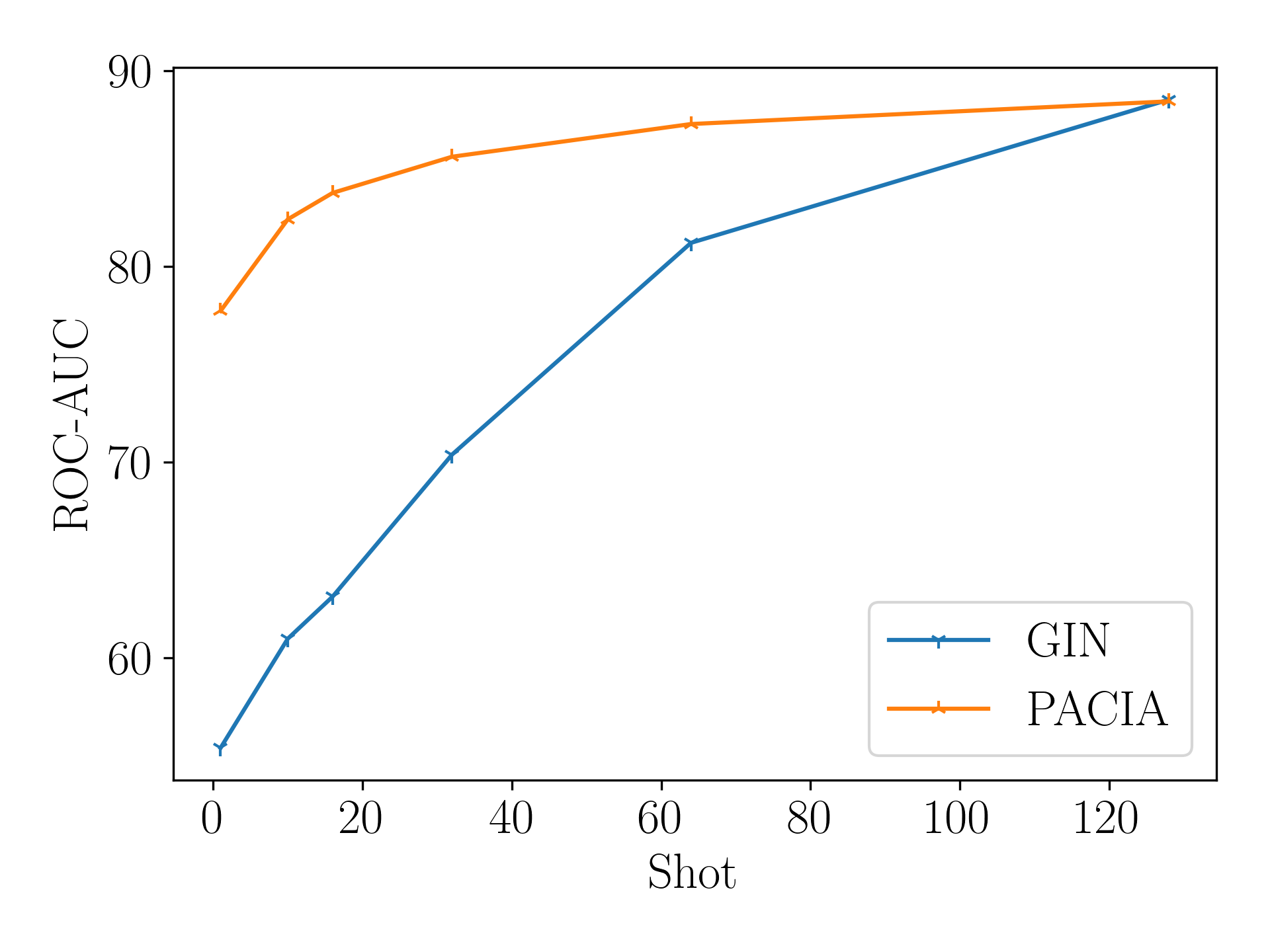
PACIA can handle general MPP problems. We conduct experiments on SIDER to validate PACIA given increasing labeled samples per task. We compare with GIN Xu et al. [2019], which is a powerful encoder to handle MPP problems. To make fair comparison, we adapt the conventional multi-task learning manner. We first train a task-shared GIN with task-specific binary classifier on all meta-training data, then inherit the GIN while use the support set of a meta-testing task to learn a task-specific classifier from scratch.
Figure 5 shows the results. As can be seen, PACIA outperforms GIN for -shot tasks, and is on par with GIN for -shot tasks. The performance gain of PACIA is more significant when fewer labeled samples are provided. Note that all parameters of GNN are fine-tuned, while PACIA only uses a few adaptive parameters to modulate the message passing process of GNN. The empirical evidence shows that PACIA nicely achieves its goal: handling few-shot MPP problem in a parameter-efficient way.
D.5 Ablation Study of Hypernetworks
For ablation studies, we provide results concerning with three aspects in hypernetworks:
Effect of Concatenating Label.
We show effect of concatenating label . Table 8 shows the testing ROC-AUC obtained on SIDER. As shown, ”w/ Label” helps keeping the label information in support set, which improves the performance.
| 10-shot | 1-shot | |
|---|---|---|
| w/ Label | ||
| w/o Label |
Different Ways of Combining Prototypes.
We show performance with different ways of combining active prototype and inactive prototype in (10) and (11). Table 9 show the results. As ”Concatenating” active and inactive prototypes allows MLP to capture more complex patterns, it obtains better performance on SIDER as shown in Table 9.
| 10-shot | 1-shot | |
|---|---|---|
| Concatenating | ||
| Mean-Pooling |
Effect of Different MLP Layers.
We show performance with different layers of MLP in hypernetworks. Table 10 shows the testing ROC-AUC obtained on SIDER. Here, we constrain that the MLPs in (9)(10)(11) have the same layer number. As shown, using 3 layers reaches the best performance. Please note that although we can set different layer numbers for MLPs used in (9)(10)(11) which further improves performance, setting the same layer number already obtains the state-of-the-art performance. Hence, we set layer number as 3 consistently.
| 1 layer | 2 layer | 3 layer | 4 layer | |
|---|---|---|---|---|
| 10-shot | ||||
| 1-shot |
D.6 A Closer Look at Query-Level Adaptation
In this section, we pay a closer look at our query-level adaptation mechanism, proving evidence of its effectiveness.
D.6.1 Performance under Different Propagation Depth
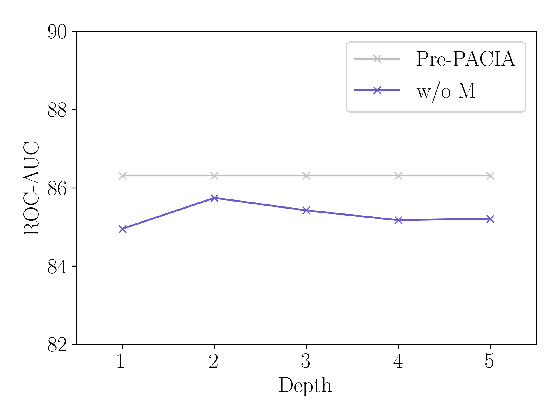
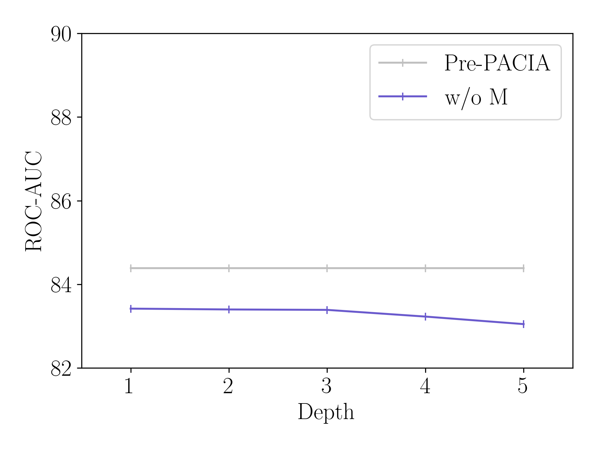
Figure 6 compares Pre-PACIA with “w/o M” (introduced in Section 5.3) using different fixed layers of relation graph refinement on Tox21, where the maximum depth . As can be seen, Pre-PACIA equipped performs much better than “w/o M” which takes the same depth of relation graph refinement as in PAR. This validates the necessity of query-level adaptation.
D.6.2 Distribution of Propagation Depth
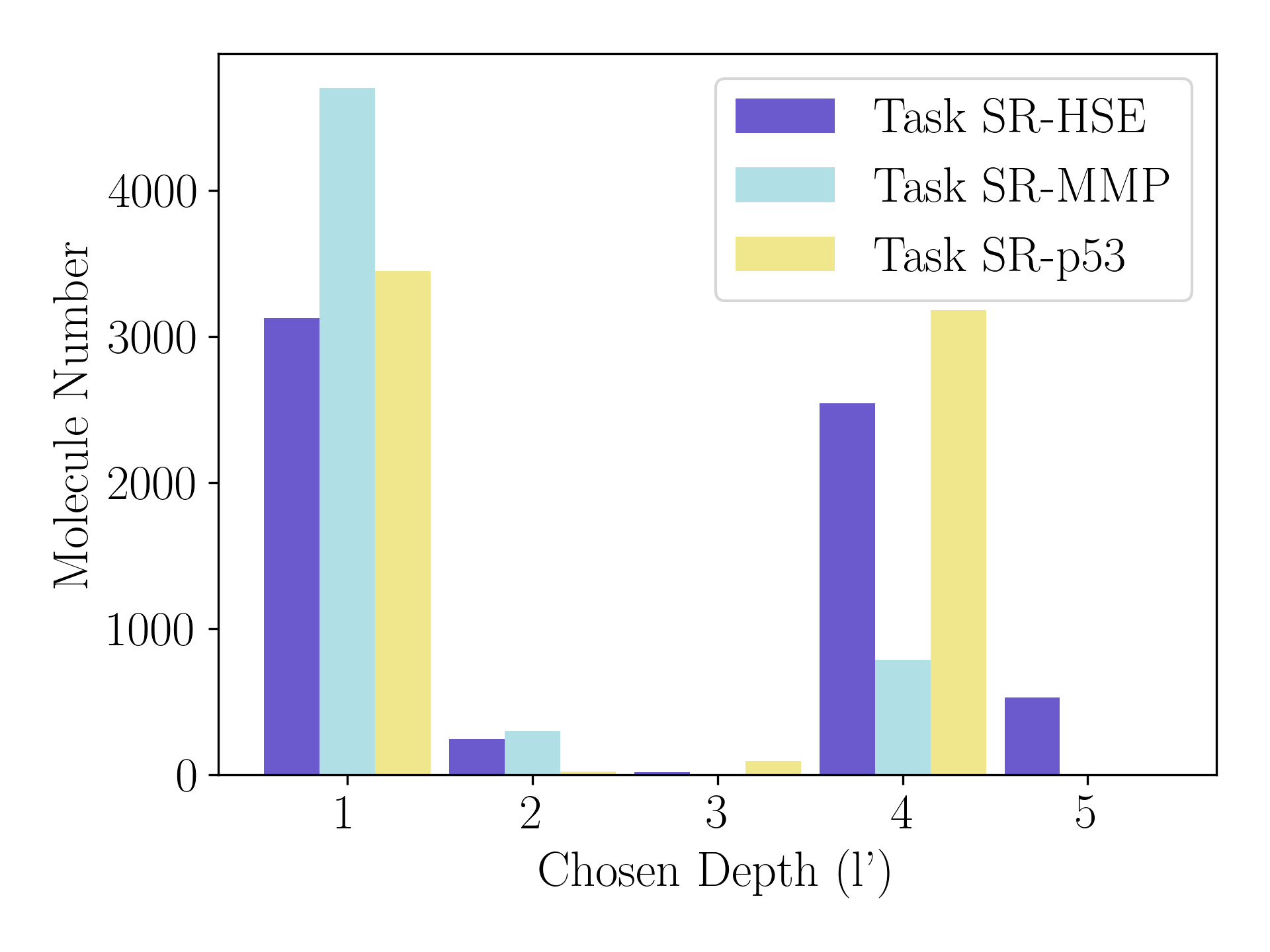
Figure 7(a) plots the distribution of learned for query molecules in meta-testing tasks for 10-shot case of Tox21. The three meta-testing tasks contain different number of query molecules in scale: 6447 in task SR-HSE, 5790 in task SR-MMP, and 6754 in task SR-p53. We can see that Pre-PACIA choose different for query molecules in the same task. Besides, the distribution of learned varies across different meta-testing tasks: molecules in task SR-MPP mainly choose smaller depth while molecules in the other two tasks tend to choose greater depth. This can be explained as most molecules in task SR-MPP are relatively easy to classify, which is consistent with the fact that Pre-PACIA obtains the highest ROC-AUC on SR-MPP among the three meta-testing tasks (83.75 for SR-HSE, 88.79 for SR-MPP and 86.39 for SR-p53).
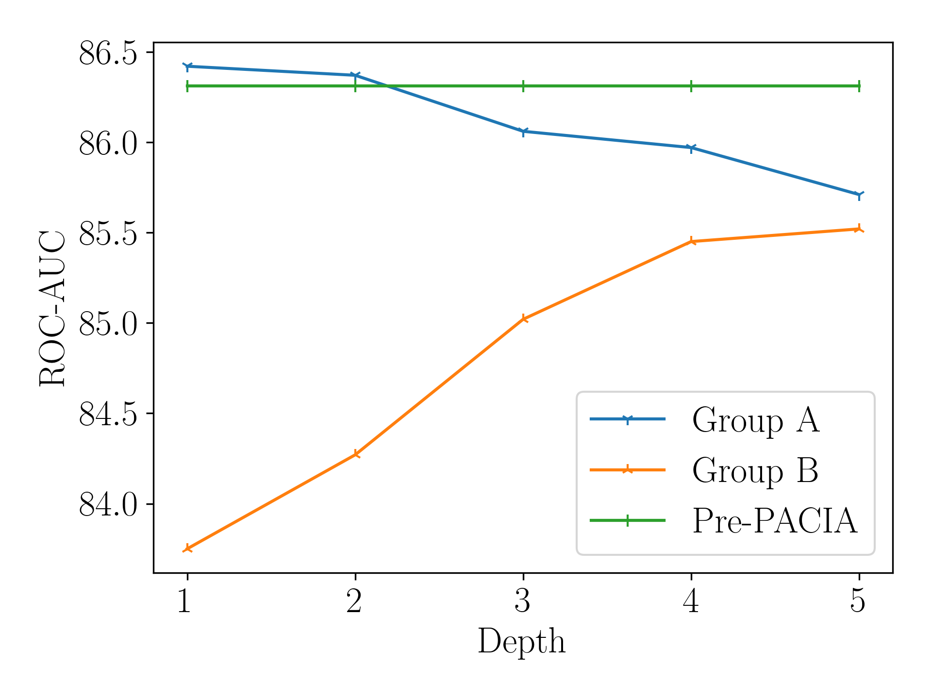
Further, we pick out molecules with (denote as Group A) and (denote as Group B) as they are more extreme cases. We then apply “w/o M” with different fixed depth for Group A and Group B, and compare them with Pre-PACIA. Figure 7(b) shows the results. Different observations can be made for these two groups. Molecules in Group A have better performance with smaller depth relation graph, they can achieve higher ROC-AUC score than the average of all molecules using Pre-PACIA. These indicate they are easier to classify and it is reasonable that Pre-PACIA choose for them. While molecules in Group B are harder to classify and require .