PairCFR: Enhancing Model Training on Paired Counterfactually Augmented Data through Contrastive Learning
Abstract
Counterfactually Augmented Data (CAD) involves creating new data samples by applying minimal yet sufficient modifications to flip the label of existing data samples to other classes. Training with CAD enhances model robustness against spurious features that happen to correlate with labels by spreading the casual relationships across different classes. Yet, recent research reveals that training with CAD may lead models to overly focus on modified features while ignoring other important contextual information, inadvertently introducing biases that may impair performance on out-of-distribution (OOD) datasets. To mitigate this issue, we employ contrastive learning to promote global feature alignment in addition to learning counterfactual clues. We theoretically prove that contrastive loss can encourage models to leverage a broader range of features beyond those modified ones. Comprehensive experiments on two human-edited CAD datasets demonstrate that our proposed method outperforms the state-of-the-art on OOD datasets.
\ul
PairCFR: Enhancing Model Training on Paired Counterfactually Augmented Data through Contrastive Learning
Xiaoqi Qiu1,*, Yongjie Wang2,*, Xu Guo2, Zhiwei Zeng2, Yue Yu2, Yuhong Feng1,†, Chunyan Miao2,† 1 Shenzhen University, 2 Nanyang Technological University 1 qiuxiaoqi2022@email.szu.edu.cn, yuhongf@szu.edu.cn 2{yongjie.wang,xu.guo,zhiwei.zeng,yue.yu,ascymiao}@ntu.edu.sg
1 Introduction
In the field of Natural Language Processing (NLP), a significant body of research McCoy et al. (2019); Wang and Culotta (2020); Poliak et al. (2018); Gururangan et al. (2018) has raised the concern that deep learning models can overfit spurious correlations, such as dataset-specific artifacts and biases, rather than focusing on the more complex, generalizable task-related features. For example, Gururangan et al. (2018) and Poliak et al. (2018) demonstrate that classifiers trained exclusively on hypotheses can still achieve decent results on some Natural Language Inference (NLI) datasets, which ideally requires comparing hypotheses with premises to determine the labels. The existence of biases or shortcuts in training datasets can severely degrade the performance of deep learning models on out-of-distribution (OOD) datasets.
Counterfactually Augmented Data (CAD) has emerged as a promising approach to mitigate this issue by making minimal modifications to existing data samples such that the corresponding labels are switched to other classes Kaushik et al. (2020); Wen et al. (2022); Pryzant et al. (2023). This technique aims to establish direct causal relationships for models to learn more effectively and enhance generalization across different datasets Teney et al. (2020); Kaushik et al. (2021).
However, the effectiveness of CAD is not always guaranteed, particularly when both contexts and the modified information should be considered together to make predictions Joshi and He (2022); Huang et al. (2020). For instance, in sentiment analysis, simply replacing positive adjectives such as “good” or “excellent” with negative counterparts like “terrible” or “bad” will potentially risk models to overemphasize these changes and even assign zero weights to the broader unmodified context Joshi and He (2022). Consequently, the trained models may fail to understand more nuanced expressions like irony or negation, exemplified by sentences such as “Is it a good movie ????” or “This movie is not that good.”
To solve the above risks of CAD training, an intuitive solution is to increase the diversity of counterfactual samples Joshi and He (2022); Sen et al. (2023), thereby disentangling the suspicious correlations between edited features and labels. Nonetheless, this kind of method often relies on human knowledge to steer the diversification, bearing high expenditure and time consumption Huang et al. (2020). Others try to design additional constraints to align the model gradient with the straight line between the counterfactual example and the original input (Teney et al., 2020), or to minimize the invariant risk (Fan et al., 2024), but these attempts fail to exploit the complex effects of augmented feature components.
In this paper, we introduce a simple yet effective learning strategy to mitigate the overfitting problem associated with CAD. Inspired by the recent success of contrastive learning (CL) in feature alignment Gao et al. (2021); Wang et al. (2022b); Liu et al. (2023a, b) and its strengths in capturing global relationships Park et al. (2023), we propose to employ a contrastive learning objective to complement the standard cross-entropy (CE) loss. While CL compels the model to extract complementary effects among counterfactually augmented data to alleviate the feature degeneration, CE ensures the induced feature representations are effectively used for classification. Our mathematical proof further corroborates the advantage of combining the two losses in training models on CAD, resulting in enhanced generation capability.
In summary, our contributions are as follows:
-
•
We introduce a contrastive learning-based framework, named Pairwisely Counterfactual Learning with Contrastive Regularization (PairCFR), for training models on CAD, which prevents overfitting to minor, non-robust edits, thus enhancing generalization performance.
-
•
We provide theoretical proof for understanding the synergistic benefits of combining the CE and CL losses, unravelling their complementary effects in preventing models from relying solely on counterfactual edits for classification.
-
•
We conduct comprehensive experiments to demonstrate that the models trained under our learning framework achieve superior OOD generalization performance on two human-edited CAD datasets.
2 Related work
Counterfactually Augmented Data. Counterfactual examples (CFEs) suggest the minimal modifications required in an input instance to elicit a different outcome Wachter et al. (2017); Barocas et al. (2020). This property has inspired researchers Kaushik et al. (2020); Wu et al. (2021) to adopt CFEs as a meaningful data augmentation in NLP, aiming to mitigate spurious correlations and improve causal learning. Early efforts Kaushik et al. (2020); Gardner et al. (2020) involved creating CAD datasets with manual sentence edits for label reversal. To ease the high cost of manual annotation, subsequent works adopt large language models (LLMs) for cost-effective generation of CAD Wu et al. (2021); Madaan et al. (2021); Wen et al. (2022); Dixit et al. (2022); Pryzant et al. (2023); Chen et al. (2023). However, findings from various investigations have indicated that training on CAD does not always ensure improved generalization on OOD tasks Huang et al. (2020); Joshi and He (2022); Fan et al. (2024). Consequently, our emphasis in this work is not on generating CAD, but rather on the exploration of methodologies to effectively utilize the inherent prior knowledge within CAD.
Contrastive Learning. Contrastive learning is initially proposed to learn a better embedding space by clustering similar samples closely while pushing dissimilar ones far apart Schroff et al. (2015); Sohn (2016); Oord et al. (2018); Wang and Isola (2020). For example, the triplet loss Schroff et al. (2015) minimizes the distance between an anchor point and its positive sample while maximizing the distance from a negative sample. The N-pair loss Sohn (2016) maximizes the distance between an anchor point with multiple negative points. Meanwhile, InfoNCE Oord et al. (2018) separates positive samples from multiple noise samples with cross-entropy loss. Enhanced by other efficient techniques, e.g., data augmentation Chen et al. (2020), hard negative sampling Schroff et al. (2015), and memory bank Wu et al. (2018), CL has propelled significant advancements in various domains, under both supervised and unsupervised settings. In this section, we explore the untapped potential of CL to enhance the OOD generalization of models trained on CAD.
Training with CAD. The task of effectively training a robust model with CAD has received relatively limited attention. The simple approach is to directly use the cross-entropy loss Kaushik et al. (2020); Wen et al. (2022); Balashankar et al. (2023). To better exploit the causal relationship in counterfactual editing, Teney et al. (2020) have introduced gradient supervision over pairs of original data and their counterfactual examples, ensuring the model gradient aligns with the straight line between the original and counterfactual points. Meanwhile, Fan et al. (2024) considers original and counterfactual distribution as two different environments and proposes a dataset-level constraint using invariant risk minimization. Following these works, we introduce a learning framework employing contrastive loss as a regularizer to enhance the generalization of fine-tuned models notably.
3 Methodology
3.1 Motivation
Recent studies have empirically shown that while perturbed features in CAD are robust and causal Kaushik et al. (2020), they may inhibit the model’s ability to learn other robust features that remain unperturbed Joshi and He (2022). In this section, we mathematically demonstrate that the standard cross-entropy loss, which is commonly used for training models on CAD, can exacerbate this tendency.
Given an instance , we train a single-layer non-linear function , where and is the sigmoid function, to predict the label . We expand , whose label , as , where denotes the features to be revised (perturbed) and denotes the constant (unperturbed) features. The counterfactual example of can be written as , with label . As the sigmoid function is monotone and bounded, the and should have different signed values to ensure that and are classified differently. We expand the weights and take it into the function to obtain and . The CE loss on the data and its counterfactual is calculated as
| (1) |
By minimizing the CE loss, we enforce to approach 1 and to approach 0. Considering that and its counterpart have different signed values, we observe that optimizing can achieve the desired contrasting effect with less effort than optimizing . Therefore, the model tends to assign higher weights for revised features and lower weights for constant or unperturbed features. An expanded illustration can be found in the Appendix A. Similar phenomena are observed in both least squares loss Joshi and He (2022) and Fisher’s Linear Discriminant on CAD Fan et al. (2024).
The above observations indicate that the CE loss alone can lead the model to focus on learning the revised features in CAD, which necessitates incorporating a regularization that compels the model to consider a broader range of features.
3.2 The Role of Contrastive Loss
Recent research findings have empirically shown that models trained under contrastive loss mainly focus on capturing global relationships Park et al. (2023) compared with negative log-likelihood losses such as masked language modeling. Inspired by this, we propose to employ CL to complement standard CE loss for training models on CAD. In the following, we start from the introduction of CL loss and then mathematically show how CL encourages the model to select a broader range of features beyond the edited ones in the counterfactual data.
Given an anchor sample from a data batch , , we have its positive samples in and negative samples in , where contains the counterfactual samples for every . The contrastive loss for the anchor is
| (2) |
where measures the cosine similarity between the hidden representations of a pair of samples, and is a temperature scaling factor for controlling the extent to which we separate positive and negative pairs Wang and Isola (2020).
Without loss of generality, we assume that directly maps the input instance into a -dimensional embedding space, . To obtain the gradient of the CL loss coming from negative samples, we have
| (3) |
The full derivation process can be found in the appendix B. Here, we have
| (4) |
which indicates the probability of being recognized as . is a symmetric matrix derived from the outer product of and . Each element of indicates the digit-level dot product between the features of and , which provides a full view of the entire feature space when comparing a pair of samples. A higher value leads to a larger gradient update and the weights are optimized by considering the whole feature sets.
The above analysis implies that the CL loss has the capability of capturing global features beyond those being edited. When learning on CAD under CL, we pair each instance with its CFE, , to compel the model to disparate from all negative samples, including its counterfactual example :
| (5) |
where the non-bold is the index of CFE. Let us revisit the toy example with and . Although minimizing the similarity between and encourages the model to focus on features , the other negative samples in the batch, e.g., , will enforce the model to use both and to compare the difference. Hence, the existence of real negative samples could help the model capture the relationships between and its context .
As all equally contribute to updating the model weights, the number of non-CFE negatives moderates the learning from local CAD and global patterns. A smaller batch size will manifest the influence of edited features, whereas a larger batch size may dilute the local differences in CAD, as discussed in the experiments 5.4.
3.3 Overall Learning Framework
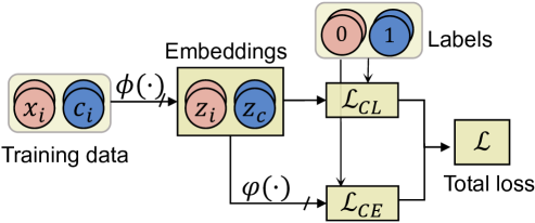
Next, we introduce our proposed learning framework, Pairwisely Counterfactual Learning with Contrastive Loss Regularization, named PairCFR for short. As shown in Figure 1, a model can be decomposed into two modules, and , i.e., , where encodes the input sentence into a hidden embedding, and maps for classification. For transformer-based models, we instantiate using the [CLS] representation, denoted as . We explicitly pair the original sentences and their CFEs, , in the same batch to provide additional training signals indicative of the underlying causal relationships.
The standard cross-entropy loss is computed on the logits vector projected from . Optimizing CE loss enforces to identify a small set of features from and assign them higher weights to quickly reach a local minimum while optimizing CL loss compels to consider the entire feature space of to meet the distance constraints. Overall, we combine the two losses as follows.
| (6) |
where is the trade-off factor to balance the two losses. To compute CL on a batch, we sample positive pairs that have the same label while all the negative samples including the CFE of the anchor sample are considered.
4 Experimental Setup
In the following, we introduce experimental settings, which include benchmark tasks, evaluation metrics, competitive baselines and implementation details. Our code is released on GitHub 111https://github.com/Siki-cloud/PairCFR.git.
4.1 Benchmark Tasks & Evaluations
We evaluate our learning framework on two NLP tasks, sentiment analysis (SA) and natural language inference (NLI). We use two human-edited CAD datasets Kaushik et al. (2020), which ensures good-quality counterfactual data Sen et al. (2023), to train all the models. The IMDb augmented dataset contains 4880 data samples with an original to CFE ratio of 1:1. The SNLI dataset contains 11330 data samples with an original to CFE ratio of 1:4. The statistics of human-revised CAD are reported in Appendix C.1.
To eliminate the random effect, we train each model for multiple runs ( runs for SA and runs for NLI) using different random seeds. We report the average test accuracy, standard deviation for both in-domain (ID) datasets and several out-of-domain (OOD) datasets. We also conduct significance tests by calculating p-value, to ensure that the observed improvements are not due to randomness. The details of ID and OOD datasets used for evaluation are described in Appendix C.2.
4.2 Implementation Details
We finetune the BERT base Devlin et al. (2019), RoBERTa base Liu et al. (2019), Sentences-BERT (SBERT, multi-qa-distilbert-cos) Reimers and Gurevych (2019) and T5 base Raffel et al. (2020) models with the original or CAD datasets on HuggingFace platform Wolf et al. (2020). Volumes of model parameters are listed in Table 7 in Appendix C.3. Following the common practices of transformers Devlin et al. (2019), we take the embedding of the “[CLS]” token as sentence representation and finetune the whole model. We set the maximum token length to 350 for SA and 64 for NLI.
We follow the original dataset splits described in Kaushik et al. (2020), where the train, validation, and test sets are divided in a ratio of 7:1:2, with all classes balanced across each set. Subsequently, we finetune all models up to 20 epochs with the AdamW optimizer, coupled with a linear learning rate scheduler with a warmup ratio as 0.05. The best learning rate is manually tuned from . We apply the early stopping strategy with a patience of and the best model is selected according to the lowest validation loss. To determine the trade-off factor and temperature , we conducted a grid search in the range with a step size of 0.1. We also conducted experiments to evaluate our PairCFR in few shot setting where the learning rate and batch size were tuned accordingly. The hyperparameters for full data finetuning and few shot setting are shown in Table 9, Table 9 respectively, in Appendix C.3.
4.3 Baselines
We compare our method PairCFR with the following baselines. For a fair comparison, we employ other forms of augmentation or increase the sampling number for the first three baselines without counterfactual augmentation, to ensure all approaches have the same number of training data.
Vanilla Devlin et al. (2019). This method refers to a general model fine-tuning with original sentences. We include this baseline to verify the improvement of our method result from both the introduction of CAD and the novel learning framework.
BTSCL Gunel et al. (2021). This approach employs the supervised contrastive loss Khosla et al. (2020) into the model training where augmented positive samples are obtained through back-translating a given sentence Ng et al. (2019).
CouCL Wang et al. (2022a). As counterexamples (CEs) are rare in a mini-batch, CouCL samples counterexamples from the original training set, where an example with lower confidence corresponds to a higher likelihood of being selected. Subsequently, it adopts the self-supervised contrastive loss to push representations of positive CEs and negative CEs far apart.
The following approaches study how to train a robust model with annotated CAD:
HCAD Kaushik et al. (2020). It collects two human-edited CAD datasets and fine-tunes a pretrained model on CAD with the cross-entropy loss.
CFGSL Teney et al. (2020). As domain priors in CAD may be lost due to random shuffling in preprocessing Kaushik et al. (2020), CFGSL pairs original data and its counterfactual example in the same batch and introduces a gradient supervision loss (GSL) alongside the cross-entropy loss. The GSL enforces the model gradient to align with the straight line from the original point to CFE.
ECF Fan et al. (2024). It introduces two additional losses to mine the causal structures of CAD. The first loss extracts the dataset-level invariance through Invariant Risk Minimization (IRM) while the second loss is applied to pairs of original sentences and CFEs, preventing the model from relying on correlated features.
| Methods | Sentiment Analysis | Natural Language Inference | |||||||||||
|---|---|---|---|---|---|---|---|---|---|---|---|---|---|
| In-Domain | Out-of-Dimain | In-Domain | Out-of-Dimain | ||||||||||
| IMDb | Amazon | Yelp | SST-2 | SNLI | MNLI-m | MNLI-mm | Negation | Spelling-e | Word-o | ||||
| BERT-base-uncased | |||||||||||||
| Vanilla | 90.15±1.66 | 86.38±0.39 | 91.03±0.83 | 81.66±0.27 | 82.59±1.00 | 85.42 | 78.85±0.44 | 57.43±0.92 | 59.36±0.80 | 40.96±4.32 | 53.56±1.54 | 50.75±6.65 | 52.41 |
| BTSCL | 90.43±1.47 | 85.45±0.71 | 91.97±0.31 | 81.79±1.28 | 83.80±1.17 | 85.75 | 79.02±0.49 | 57.28±1.30 | 59.10±1.42 | 43.10±3.65 | 53.51±1.74 | 49.20±4.51 | 52.44 |
| CouCL | 85.67±1.13 | 86.75±0.22 | 89.53±0.55 | 84.41±0.23 | 85.01±0.43 | 86.43 | 71.90±0.95 | 51.99±1.75 | 52.20±1.86 | 38.70±4.69 | 49.82±2.01 | 44.03±4.02 | 47.35 |
| HCAD | 88.16±2.70 | 86.40±0.77 | 89.94±0.99 | 83.29±2.71 | 85.74±1.04 | 86.34 | 73.49±1.37 | 58.53±1.59 | 60.77±1.46 | 35.43±3.06 | 54.01±2.70 | 54.72±3.29 | 52.69 |
| CFGSL | 88.51±3.29 | 85.52±1.05 | 89.58±1.83 | 84.56±1.53 | 86.77±0.79 | 86.61 | 77.16±0.41 | 60.11±1.07 | 62.25±0.66 | 33.81±1.89 | 56.37±0.74 | 58.45±0.97 | 54.20 |
| ECF | 87.71±0.29 | 86.43±0.10 | 89.30±0.16 | 83.05±0.69 | 86.23±0.18 | 86.25 | 73.23±1.52 | 58.95±0.15 | 61.19±1.34 | 42.40±1.07 | 54.15±0.53 | 57.10±0.92 | 54.76 |
| Ours | 89.63±1.36 | 86.79±0.72 | 91.78±0.44 | 85.27±0.39 | 86.81±0.97 | 87.66 | 75.38±0.21 | 60.46±0.38 | 62.27±0.39 | 39.21±3.61 | 56.84±0.54 | 59.16±0.88 | 55.59 |
| RoBERTa-base | |||||||||||||
| Vanilla | 92.68±1.15 | 87.08±1.39 | 94.00±0.77 | 81.43±2.82 | 86.04±2.76 | 87.14 | 85.16±0.39 | 70.35±1.29 | 71.25±1.59 | 52.47±5.55 | 67.36±1.36 | 61.82±4.54 | 64.65 |
| BTSCL | 93.09±0.61 | 89.46±0.21 | 94.74±0.36 | 85.72±1.22 | 87.16±0.87 | 89.27 | 85.72±0.44 | 70.83±1.38 | 72.10±1.32 | 56.89±3.78 | 67.61±1.32 | 62.22±3.55 | 65.93 |
| CouCL | 91.22±0.83 | 89.48±0.19 | 93.04±0.58 | 87.40±0.77 | 88.07±0.66 | 89.50 | 82.37±0.52 | 70.86±1.32 | 71.38±1.23 | 51.83±2.71 | 68.08±1.23 | 64.68±1.82 | 65.37 |
| HCAD | 90.12±1.74 | 88.50±0.57 | 92.18±0.94 | 83.43±1.75 | 86.48±0.98 | 87.65 | 80.91±0.69 | 70.35±1.08 | 70.77±0.76 | 45.79±4.16 | 67.37±1.28 | 64.83±1.47 | 63.82 |
| CFGSL | 90.69±0.92 | 88.32±0.41 | 93.48±0.48 | 83.90±1.78 | 86.89±0.80 | 88.15 | 82.45±0.35 | 71.59±0.90 | 71.25±1.06 | 51.40±1.47 | 68.86±1.07 | 62.22±1.99 | 65.06 |
| ECF | 91.05±0.44 | 88.56±0.32 | 93.79±0.19 | 85.82±0.43 | 87.84±0.59 | 89.00 | 81.88±0.17 | 70.45±1.03 | 71.18±0.93 | 51.70±2.38 | 66.60±0.94 | 63.76±1.98 | 64.74 |
| Ours | 91.74±0.88 | 89.60±0.26 | 93.35±0.34 | 87.90±0.45 | 88.61±0.41 | 89.87 | 82.13±0.51 | 71.80±0.53 | 72.12±0.79 | 55.19±1.97 | 68.88±0.36 | 65.91±1.35 | 66.78 |
| SBERT-multi-qa-distilbert-cos | |||||||||||||
| Vanilla | 87.61±1.86 | 80.65±0.67 | 89.74±0.77 | 83.95±1.12 | 82.01±1.59 | 84.09 | 76.96±0.53 | 53.90±2.03 | 55.90±2.22 | 45.20±4.18 | 51.23±2.72 | 48.27±5.00 | 50.90 |
| BTSCL | 88.84±2.41 | 81.21±0.76 | 90.49±0.37 | 84.20±0.61 | 83.62±0.64 | 84.88 | 77.16±0.38 | 54.42±1.31 | 56.14±1.36 | 45.40±2.78 | 52.44±1.83 | 49.80±2.63 | 51.64 |
| CouCL | 87.96±0.67 | 83.92±0.13 | 89.15±0.18 | 85.40±0.31 | 83.48±0.37 | 85.49 | 70.61±1.54 | 55.29±1.45 | 57.90±1.81 | 35.86±1.87 | 52.01±2.26 | 54.89±1.91 | 51.19 |
| HCAD | 86.09±1.74 | 83.94±0.39 | 87.87±0.66 | 85.91±0.66 | 82.83±0.90 | 85.14 | 71.64±1.04 | 55.93±1.61 | 58.70±1.96 | 35.05±1.22 | 53.33±1.06 | 54.86±2.08 | 51.57 |
| CFGSL | 86.05±1.07 | 82.71±0.73 | 87.59±0.75 | 83.36±0.55 | 83.70±0.49 | 84.34 | 70.72±1.06 | 55.84±0.88 | 58.52±1.15 | 36.07±3.38 | 52.60±1.27 | 55.57±1.68 | 51.72 |
| ECF | 87.83±0.46 | 84.51±0.34 | 88.44±0.20 | 84.60±0.70 | 84.27±0.56 | 85.46 | 64.55±1.23 | 49.95±1.84 | 51.49±1.82 | 38.59±2.32 | 48.31±1.67 | 49.55±2.27 | 47.58 |
| Ours | 87.28±0.75 | 84.58±0.22 | 88.52±0.30 | 86.32±0.35 | 84.31±0.78 | 85.93 | 71.48±0.40 | 57.19±0.84 | 60.76±0.46 | 37.27±2.35 | 54.36±0.67 | 56.78±1.24 | 53.27 |
| T5-base | |||||||||||||
| Vanilla | 92.15±1.49 | 88.24±0.85 | 94.44±0.67 | 83.40±1.38 | 86.17±2.60 | 88.06 | 83.28±0.57 | 62.62±2.59 | 65.18±2.10 | 41.00±2.46 | 58.76±2.61 | 48.30±3.27 | 55.17 |
| BTSCL | 92.78±1.08 | 88.50±0.81 | 94.89±0.42 | 83.37±1.09 | 87.17±1.07 | 88.48 | 83.66±0.46 | 64.01±2.57 | 66.47±2.24 | 42.16±2.90 | 60.01±3.43 | 50.16±5.69 | 56.56 |
| CouCL | 91.74±0.88 | 88.91±0.47 | 93.35±0.34 | 87.03±0.70 | 88.61±0.41 | 89.48 | 79.81±0.54 | 70.19±0.58 | 71.84±0.76 | 39.82±3.23 | 66.35±0.68 | 64.29±1.58 | 62.50 |
| HCAD | 90.09±1.95 | 88.72±0.85 | 92.60±0.87 | 85.63±1.15 | 85.54±1.28 | 88.12 | 80.09±0.73 | 70.19±0.72 | 71.60±0.83 | 45.05±3.94 | 66.57±0.73 | 65.30±1.51 | 63.74 |
| CFGSL | 89.48±5.17 | 88.27±1.05 | 92.77±1.45 | 81.56±2.49 | 82.11±2.50 | 86.18 | 80.71±0.64 | 69.08±0.97 | 69.85±1.12 | 45.59±3.74 | 65.58±1.18 | 65.80±1.55 | 63.18 |
| ECF | 90.85±0.37 | 89.27±0.25 | 92.65±0.44 | 87.66±0.26 | 88.57±0.54 | 89.54 | 78.93±0.51 | 69.57±1.14 | 70.30±1.45 | 46.14±3.12 | 64.19±1.08 | 65.79±1.71 | 63.20 |
| Ours | 91.47±0.89 | 89.18±0.21 | 93.45±0.63 | 87.90±0.45 | 88.64±1.04 | 89.79 | 80.87±0.77 | 71.38±0.13 | 72.46±0.57 | 46.31±0.50 | 67.37±0.12 | 67.39±0.33 | 64.98 |
| Sentiment Analysis | Natural Language Inference | |||||||||||||
| Variants | In-Domain | Out-of-Dimain | In-Domain | Out-of-Dimain | ||||||||||
| #Train | Loss | IMDb | Amazon | Yelp | SST-2 | SNLI | MNLI-m | MNLI-mm | Negation | Spelling-e | Word-o | |||
| BERT-base-uncased | ||||||||||||||
| ShuffCAD | CE | 88.16±2.70 | 86.40±0.77 | 89.94±0.99 | 83.29±2.71 | 85.74±1.04 | 86.34 | 73.49±1.37 | 58.53±1.59 | 60.77±1.46 | 35.43±3.06 | 54.01±2.70 | 54.72±3.29 | 52.69 |
| PairCAD | CE | 88.23±3.11 | 86.56±0.34 | 89.97±1.85 | 84.15±1.20 | 85.84±0.85 | 86.62 | 74.27±0.72 | 59.13±0.65 | 60.85±0.88 | 36.10±1.92 | 56.14±1.34 | 55.40±2.83 | 53.52 |
| ShuffCAD | CE+CL | 89.18±1.33 | 86.77±0.65 | 91.45±0.53 | 84.14±1.82 | 86.26±0.99 | 87.15 | 73.77±1.11 | 59.39±0.64 | 61.85±0.86 | 36.80±4.04 | 55.62±0.87 | 57.09±2.45 | 54.15 |
| PairCAD | CE+CL | 89.63±1.36 | 86.79±0.72 | 91.78±0.44 | 85.27±0.39 | 86.81±0.97 | 87.66 | 75.38±0.21 | 60.46±0.38 | 62.27±0.39 | 39.21±3.61 | 56.84±0.54 | 59.16±0.88 | 55.59 |
| RoBERTa-base | ||||||||||||||
| ShuffCAD | CE | 90.12±1.74 | 88.50±0.57 | 92.18±0.94 | 83.43±1.75 | 86.48±0.98 | 87.67 | 80.91±0.69 | 70.35±1.08 | 70.77±0.76 | 45.79±4.16 | 67.37±1.28 | 64.83±1.47 | 63.82 |
| PairCAD | CE | 90.95±0.84 | 88.77±0.74 | 92.77±0.95 | 83.45±2.53 | 86.37±1.06 | 87.84 | 81.69±0.90 | 70.77±0.49 | 71.33±0.45 | 54.38±1.67 | 67.90±0.63 | 65.43±0.99 | 65.96 |
| ShuffCAD | CE+CL | 91.42±1.01 | 89.44±0.27 | 92.91±0.64 | 86.67±1.05 | 87.25±0.68 | 89.07 | 81.95±0.39 | 71.16±0.60 | 71.79±0.79 | 51.43±2.91 | 68.20±0.57 | 64.12±1.03 | 65.34 |
| PairCAD | CE+CL | 91.74±0.88 | 89.60±0.26 | 93.35±0.34 | 87.90±0.45 | 88.61±0.41 | 89.61 | 82.13±0.51 | 71.80±0.53 | 72.12±0.79 | 55.19±1.97 | 68.88±0.36 | 65.91±1.35 | 66.78 |
| SBERT-multi-qa-distilbert-cos | ||||||||||||||
| ShuffCAD | CE | 86.09±1.74 | 83.94±0.39 | 87.87±0.66 | 85.91±0.66 | 82.83±0.90 | 85.13 | 71.64±1.04 | 55.93±1.61 | 58.70±1.96 | 35.05±1.22 | 53.33±1.06 | 54.86±2.08 | 51.57 |
| PairCAD | CE | 86.78±1.41 | 83.55±0.39 | 88.51±0.77 | 85.95±0.40 | 83.20±0.63 | 85.30 | 70.90±1.02 | 56.50±0.58 | 59.03±0.57 | 35.89±1.98 | 53.03±1.17 | 55.04±1.03 | 51.89 |
| ShuffCAD | CE+CL | 87.68±1.05 | 84.23±0.37 | 88.66±0.77 | 85.45±0.28 | 83.60±0.38 | 85.48 | 71.38±0.62 | 57.08±0.53 | 60.01±0.35 | 35.11±1.64 | 54.15±0.53 | 55.59±1.89 | 52.39 |
| PairCAD | CE+CL | 87.28±0.22 | 84.58±0.22 | 88.52±0.30 | 86.32±0.35 | 84.31±0.7 | 85.93 | 71.48±0.40 | 57.19±0.84 | 60.76±0.46 | 37.27±2.35 | 54.36±0.67 | 56.78±1.24 | 53.27 |
| T5-base | ||||||||||||||
| ShuffCAD | CE | 90.09±1.95 | 88.72±0.85 | 92.60±0.87 | 85.63±1.15 | 85.54±1.28 | 88.12 | 80.09±0.73 | 70.19±0.72 | 71.60±0.83 | 45.05±3.94 | 66.57±0.73 | 65.30±1.51 | 63.85 |
| PairCAD | CE | 90.03±1.35 | 89.02±0.41 | 92.76±0.99 | 86.46±1.00 | 86.59±1.37 | 88.71 | 79.55±0.66 | 68.86±0.52 | 70.75±0.77 | 45.18±3.49 | 65.56±0.67 | 65.64±1.50 | 62.83 |
| ShuffCAD | CE+CL | 90.38±1.80 | 89.03±0.46 | 93.06±1.29 | 85.75±0.96 | 87.24±2.12 | 88.76 | 80.21±0.10 | 70.43±0.11 | 71.78±0.37 | 45.41±2.08 | 66.59±0.56 | 66.28±0.93 | 64.09 |
| PairCAD | CE+CL | 91.47±0.89 | 89.18±0.21 | 93.45±0.63 | 87.03±0.70 | 88.64±1.04 | 89.79 | 80.87±0.77 | 71.38±0.13 | 72.46±0.57 | 46.31±0.50 | 67.37±0.12 | 67.39±0.33 | 64.98 |
| Train Data | netural samples | In-Domain | Out-of-Dimain | |||||
|---|---|---|---|---|---|---|---|---|
| SNLI | MNLI-m | MNLI-mm | Negation | Spelling-e | Word-o | |||
| PairCAD | w | 73.29±1.09 | 59.41±0.91 | 61.66±0.85 | 35.96±2.81 | 56.42±1.10 | 56.14±2.60 | 53.92 |
| PairCAD | w/o | 75.38±0.21 | 60.46±0.38 | 62.27±0.39 | 39.21±3.61 | 56.84±0.54 | 59.16±0.88 | 55.59 |
| p-value | 5.90e-06 | 0.0109 | 0.0055 | 0.0053 | 0.0087 | 0.0107 | - | |
| In-Domain | Out-of-Domain | |||||||
|---|---|---|---|---|---|---|---|---|
| Train Data CE+CL | R:O | SNLI | MNLI-m | MNLI-mm | Negation | Spelling-e | Word-o | |
| Original (20k) | - | 85.09±0.27 | 69.53±1.38 | 71.62±1.04 | 45.65±3.53 | 66.43±1.49 | 52.89±5.22 | 61.22 |
| PairCAD (3.3k) | 1 | 74.50±2.51 | 65.24±1.63 | 67.61±1.36 | 38.38±3.42 | 61.24±1.86 | 60.61±2.33 | 58.62 |
| PairCAD (4.9k) | 2 | 76.12±1.58 | 66.62±1.05 | 69.31±0.87 | 42.33±7.31 | 62.91±1.60 | 62.61±1.58 | 60.76 |
| PairCAD (6.4k) | 3 | 77.98±0.82 | 68.36±1.48 | 70.00±1.44 | 43.13±1.17 | 64.60±1.98 | 64.45±2.15 | 62.11 |
| PairCAD (8.3k) | 4 | 80.14±0.96 | 71.02±0.39 | 71.84±0.76 | 45.73±0.70 | 66.87±0.51 | 67.11±0.39 | 64.51 |
5 Results and Analysis
5.1 Overall Performance Comparison
Table 1 reports the overall performance comparisons, showing that our proposed PairCFR method outperforms all the baseline models on three out of four OOD datasets for both SA and NLI tasks across four different backbone models. To exclude the possibility of marginal improvements due to random initializations, we also conducted significance tests under the null hypothesis that there are no differences between each baseline and our approach, as presented in Table 11, located in Appendix C.6. The p-values less than demonstrate that our methods are significantly better than the baselines, even though some improvements are relatively slight in Table 1.
In addition, we reported the following findings. Firstly, CAD-based methods may perform worse than non-CAD methods on OOD tasks, e.g., HCAD always lags behind CouCL on the SA task using fine-tuned T5 model. A similar phenomenon is also reported in Joshi and He (2022). These could be due to the failure to extract complementary features between CFEs and the original data; Secondly, the introduction of CFEs may shift the training data distribution from the in-domain data distribution. As anticipated, CAD-based methods fall behind non-CAD methods on ID datasets. Thirdly, our proposed PairCFR exhibits superior OOD performance compared to the baselines, achieving the highest accuracy on mostly OOD datasets, with the sole exceptions being the Yelp and Negation datasets. We postulate that the noted exceptions may be attributed to Yelp and Negative datasets having distributions similar to the ID datasets. The above results validate that PairCFR possesses a heightened capability to learn prior knowledge in CAD.
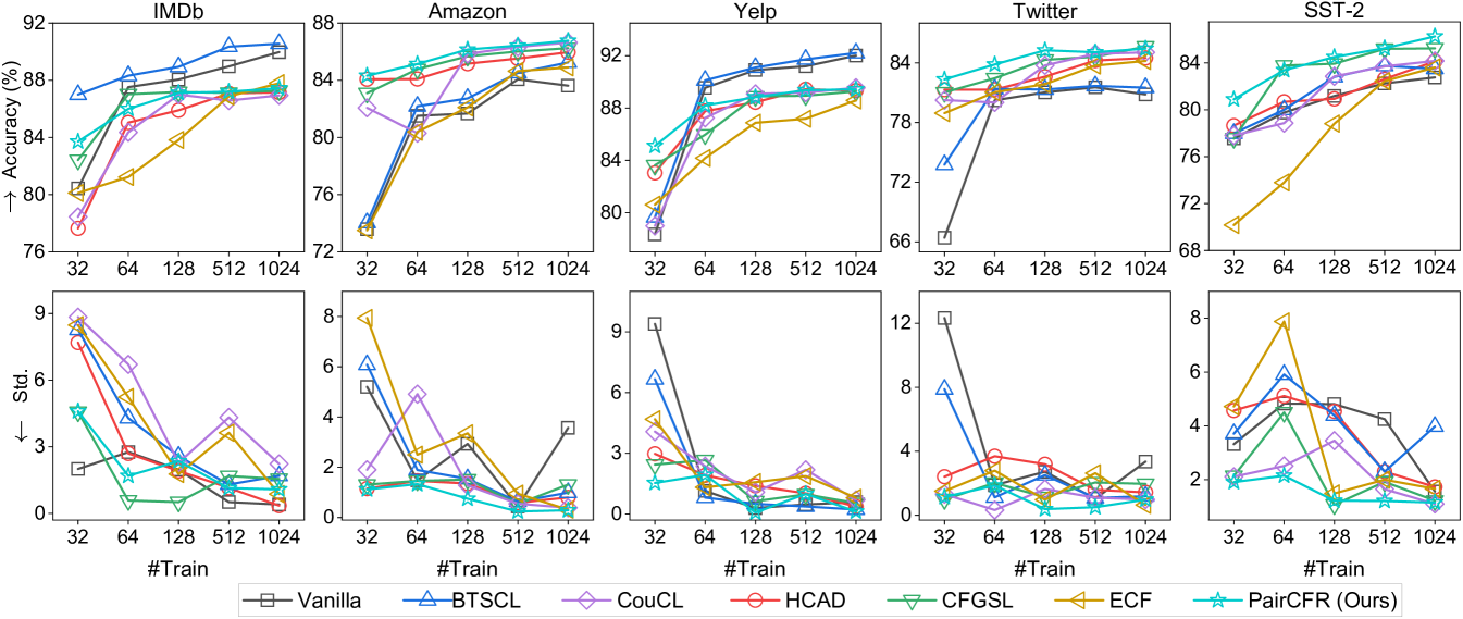
5.2 Few-shot Learning Performance
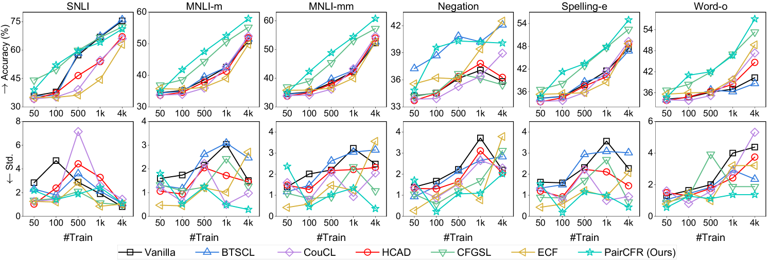
Data augmentation, such as counterfactual augmentation, is frequently utilized to enhance the performance of few-shot learning. In this part, we investigate the effectiveness of our proposed PairCFR in few-shot learning scenarios. We conducted experiments using the finetuned BERTbase model on the SNLI dataset, gradually increasing the number of training samples from 50 to 4,000. Similarly, on the IMDB dataset, we increased the number of training samples from 32 to 1,024.
Experiment results on SNLI and IMDB under the few-shot setting are reported in Figure 2 and Figure 5 ( Appendix C.5). From both tables, we can conclude that our PairCFR generally demonstrates higher accuracy and lower standard deviation across OOD datasets, particularly in scenarios where training sample sizes are small. For instance, PairCFR significantly outperforms other methods by around 6% on Spelling-e when trained with only 100 counterfactually augmented samples.
5.3 Ablation Study
We conducted ablation experiments to verify the efficacy of two crucial strategies of our proposed method: (1) the pairing strategy: the integration of original data with their CFEs within the same batch, denoted PairCAD, versus ShuffCAD where randomly shuffle CFEs and originals. (2) the CL loss: the incorporation of CL and CE loss versus CE loss alone.
Results in Table 2, together with significance tests in Table 11 in Appendix C.6, offer several insights: 1) The strategy of pairing original data with their CFEs in the same batch improves OOD performance for both SA and NLI tasks. This can be attributed to the preservation of prior causal relations, which might be lost during random shuffling; 2) The efficacy of PairCAD with a CE-alone learning framework is not guaranteed. For example, within the T5 model framework, PairCAD underperforms ShuffCAD on the SNLI, MNLI, and Spelling-e datasets when only CE loss is adopted. This underscores the critical role of the CL component in augmenting features when we batch CFEs and original data; 3) Integrating the CL consistently improves model performance in both ID and OODs. Particularly, combining CL with PairCAD yields the best performance across various model assessments, highlighting the effectiveness of contrastive learning and the pairing strategy in leveraging causal relations of CFEs.
5.4 Impact of Batch Size
In this study, we investigated the effect of batch size on learning performance. We conducted experiments on the fine-tuned BERT model for SA and the fine-tuned T5 model for NLI, incrementally increasing the batch size while maintaining the original augmentation ratio for each task. From Figure LABEL:fig:batchsize, we observe that the model performance on both tasks initially improves with increasing batch size, but eventually reaches a plateau or experiences a slight decline.
We contend that the inclusion of negative samples in the CL function provides additional regularization, forcing the model to rely on a broader array of features beyond those edited. However, an excessively large batch size introduces an overwhelming number of negative samples in CL, which may dilute the human priors in CAD, leading to diminished performance. This trend is consistent across both SA and NLI tasks, highlighting the effort required in batch size selection.
5.5 Contribution of Neutral Class in NLI
Do all counterfactual examples equivalently contribute to enhancing model generality? To answer this, we specifically experimented with the fine-tuned BERT model on the NLI task, comparing performance with and without the inclusion of neutral class samples in CL.
Results in Table 4 reveal that removing neutral samples, including neutral CFEs, significantly enhances the OOD generalization by approximately 2% when training the model on CAD with our learning framework. We attribute this performance difference to the distinct nature of neutral samples. In NLI tasks, judgments of entailment and contradiction are often readily determined based on the semantic alignment or disparity between text elements. Conversely, neutral samples represent scenarios where the hypothesis and premise lack any clear relationship, encompassing a vast array of potential expressions. This diversity poses a great challenge for models to identify universal patterns within the neutral class through human annotations. Therefore, adding neutral samples into the CL detrimentally affects the model’s performance in our experiments.
This investigation highlights the necessity of contemplating the practical value of adding additional counterfactual examples for specific classes.
5.6 Effect of Counterfactual Diversity
We also investigated the role of CFE diversity in improving model performance on the NLI task. In SNLI, each sentence is annotated with CFEs, due to the existence of two opposite targets and modifications made to both the hypothesis and premise. Each CFE is obtained through a different type of modification, resulting in a dataset that includes more diverse counterfactuals. We fine-tuned the T5base model by incrementally including more CFEs in a batch, ranging from to .
The results in Table 4, reveal a direct relation between the number of CFEs and the model’s generalization capabilities. Notably, the OOD performance of the model trained on CAD is even better than that trained on a times larger dataset with only original data. We conclude that enhancing counterfactual diversity proves to be an efficient strategy, which is the same as the findings reported in Joshi and He (2022).
6 Conclusion
Counterfactually Augmented Data (CAD) can enhance model robustness by explicitly identifying causal features. However, recent research found that CAD may fall behind non-CAD methods on generality. In this work, we introduce PairCFR to overcome this challenge. PairCFR pairs original and counterfactual data during training and includes both contrastive and cross-entropy losses for learning discriminative representations. We prove that contrastive loss aids models in capturing sufficient relationships not represented in CAD, thus improving generality. Extensive experiments demonstrate that our PairCFR achieves superior accuracy and robustness in various scenarios. Our findings emphasize the potential of carefully designed training paradigms in utilization of CAD.
7 Limitations
Our PairCFR has been demonstrated to effectively improve models’ OOD generalization with human-edited CAD datasets, which, despite its high quality, is quite limited in size. Future work will focus on utilizing LLMs such as ChatGPT or GPT-4 to generate a larger volume of CAD. Yet, LLM-generated CAD may suffer from lower quality due to noisy and insufficient perturbations. It remains crucial and necessary to extend our PairCFR framework to accommodate such compromised CAD. Furthermore, PairCFR currently utilizes a simple form of contrastive loss, namely InfoNCE. In the future, we aim to investigate alternative contrastive loss variants and assess their potential to further enhance OOD generalization capabilities. Lastly, our experiments were conducted using relatively older and moderately sized LLMs, such as BERT and RoBERTa. We are also interested in exploring the potential improvements on larger LLMs by employing parameter-efficient finetuning methods.
8 Ethics Statement
This work focuses on reducing shortcut learning in models trained on CAD, thereby improving their robustness and generalization. Similar to other methods designed to mitigate learning from spurious correlations, our proposed PairCFR could help elicit trust in NLP models. It assists models in better-considering context (see Section 3 for details), preventing decision-making based on incomplete or biased information, such as solely on the edited words in CAD. Nonetheless, ensuring absolute fairness in model decisions in complex real-world contexts remains a formidable challenge solely from a model design standpoint. For instance, models could be compromised by low-quality or erroneous counterfactual data, leading to the learning of false relationships and resulting in erroneous or biased real-world decisions. Consequently, it is crucial for practitioners to consider the quality of counterfactual data alongside model design.
Acknowledgements
This research is supported, in part, by the Joint NTU-WeBank Research Centre on Fintech, Nanyang Technological University, Singapore. This research is supported, in part, by the National Research Foundation, Prime Minister’s Office, Singapore under its NRF Investigatorship Programme (NRFI Award No. NRF-NRFI05-2019-0002). Any opinions, findings and conclusions or recommendations expressed in this material are those of the author(s) and do not reflect the views of National Research Foundation, Singapore. Xu Guo wants to thank the Wallenberg-NTU Presidential Postdoctoral Fellowship. Zhiwei Zeng thanks the support from the Gopalakrishnan-NTU Presidential Postdoctoral Fellowship. This research is also supported by the Shenzhen Science and Technology Foundation (General Program, JCYJ20210324093212034) and the 2022 Guangdong Province Undergraduate University Quality Engineering Project (Shenzhen University Academic Affairs [2022] No. 7). We also appreciate the support from Guangdong Province Key Laboratory of Popular High Performance Computers 2017B030314073, Guangdong Province Engineering Center of China-made High Performance Data Computing System.
References
- Balashankar et al. (2023) Ananth Balashankar, Xuezhi Wang, Yao Qin, Ben Packer, Nithum Thain, Ed Chi, Jilin Chen, and Alex Beutel. 2023. Improving classifier robustness through active generative counterfactual data augmentation. In Findings of the Association for Computational Linguistics: EMNLP 2023, pages 127–139, Singapore. Association for Computational Linguistics.
- Barocas et al. (2020) Solon Barocas, Andrew D Selbst, and Manish Raghavan. 2020. The hidden assumptions behind counterfactual explanations and principal reasons. In Proceedings of the 2020 conference on fairness, accountability, and transparency, pages 80–89.
- Bowman et al. (2015) Samuel R. Bowman, Gabor Angeli, Christopher Potts, and Christopher D. Manning. 2015. A large annotated corpus for learning natural language inference. In Proceedings of the 2015 Conference on Empirical Methods in Natural Language Processing, pages 632–642, Lisbon, Portugal. Association for Computational Linguistics.
- Chen et al. (2020) Ting Chen, Simon Kornblith, Mohammad Norouzi, and Geoffrey Hinton. 2020. A simple framework for contrastive learning of visual representations. In International conference on machine learning, pages 1597–1607. PMLR.
- Chen et al. (2023) Zeming Chen, Qiyue Gao, Antoine Bosselut, Ashish Sabharwal, and Kyle Richardson. 2023. DISCO: Distilling counterfactuals with large language models. In Proceedings of the 61st Annual Meeting of the Association for Computational Linguistics (Volume 1: Long Papers), pages 5514–5528, Toronto, Canada. Association for Computational Linguistics.
- Devlin et al. (2019) Jacob Devlin, Ming-Wei Chang, Kenton Lee, and Kristina Toutanova. 2019. BERT: Pre-training of deep bidirectional transformers for language understanding. In Proceedings of the 2019 Conference of the North American Chapter of the Association for Computational Linguistics: Human Language Technologies, Volume 1 (Long and Short Papers), pages 4171–4186, Minneapolis, Minnesota. Association for Computational Linguistics.
- Dixit et al. (2022) Tanay Dixit, Bhargavi Paranjape, Hannaneh Hajishirzi, and Luke Zettlemoyer. 2022. CORE: A retrieve-then-edit framework for counterfactual data generation. In Findings of the Association for Computational Linguistics: EMNLP 2022, pages 2964–2984, Abu Dhabi, United Arab Emirates. Association for Computational Linguistics.
- Fan et al. (2024) Caoyun Fan, Wenqing Chen, Jidong Tian, Yitian Li, Hao He, and Yaohui Jin. 2024. Unlock the potential of counterfactually-augmented data in out-of-distribution generalization. Expert Systems with Applications, 238:122066.
- Gao et al. (2021) Tianyu Gao, Xingcheng Yao, and Danqi Chen. 2021. SimCSE: Simple contrastive learning of sentence embeddings. In Proceedings of the 2021 Conference on Empirical Methods in Natural Language Processing, pages 6894–6910, Online and Punta Cana, Dominican Republic. Association for Computational Linguistics.
- Gardner et al. (2020) Matt Gardner, Yoav Artzi, Victoria Basmov, Jonathan Berant, Ben Bogin, Sihao Chen, Pradeep Dasigi, Dheeru Dua, Yanai Elazar, Ananth Gottumukkala, Nitish Gupta, Hannaneh Hajishirzi, Gabriel Ilharco, Daniel Khashabi, Kevin Lin, Jiangming Liu, Nelson F. Liu, Phoebe Mulcaire, Qiang Ning, Sameer Singh, Noah A. Smith, Sanjay Subramanian, Reut Tsarfaty, Eric Wallace, Ally Zhang, and Ben Zhou. 2020. Evaluating models’ local decision boundaries via contrast sets. In Findings of the Association for Computational Linguistics: EMNLP 2020, pages 1307–1323, Online. Association for Computational Linguistics.
- Gunel et al. (2021) Beliz Gunel, Jingfei Du, Alexis Conneau, and Veselin Stoyanov. 2021. Supervised contrastive learning for pre-trained language model fine-tuning. In International Conference on Learning Representations.
- Gururangan et al. (2018) Suchin Gururangan, Swabha Swayamdipta, Omer Levy, Roy Schwartz, Samuel Bowman, and Noah A. Smith. 2018. Annotation artifacts in natural language inference data. In Proceedings of the 2018 Conference of the North American Chapter of the Association for Computational Linguistics: Human Language Technologies, Volume 2 (Short Papers), pages 107–112, New Orleans, Louisiana. Association for Computational Linguistics.
- Huang et al. (2020) William Huang, Haokun Liu, and Samuel R. Bowman. 2020. Counterfactually-augmented SNLI training data does not yield better generalization than unaugmented data. In Proceedings of the First Workshop on Insights from Negative Results in NLP, pages 82–87, Online. Association for Computational Linguistics.
- Joshi and He (2022) Nitish Joshi and He He. 2022. An investigation of the (in)effectiveness of counterfactually augmented data. In Proceedings of the 60th Annual Meeting of the Association for Computational Linguistics (Volume 1: Long Papers), pages 3668–3681, Dublin, Ireland. Association for Computational Linguistics.
- Kaushik et al. (2020) Divyansh Kaushik, Eduard Hovy, and Zachary C Lipton. 2020. Learning the difference that makes a difference with counterfactually augmented data. International Conference on Learning Representations (ICLR).
- Kaushik et al. (2021) Divyansh Kaushik, Amrith Setlur, Eduard Hovy, and Zachary C Lipton. 2021. Explaining the efficacy of counterfactually augmented data. International Conference on Learning Representations (ICLR).
- Khosla et al. (2020) Prannay Khosla, Piotr Teterwak, Chen Wang, Aaron Sarna, Yonglong Tian, Phillip Isola, Aaron Maschinot, Ce Liu, and Dilip Krishnan. 2020. Supervised contrastive learning. Advances in neural information processing systems, 33:18661–18673.
- Liu et al. (2023a) Meizhen Liu, Xu Guo, He Jiakai, Jianye Chen, Fengyu Zhou, and Siu Hui. 2023a. InteMATs: Integrating granularity-specific multilingual adapters for cross-lingual transfer. In Findings of the Association for Computational Linguistics: EMNLP 2023, pages 5035–5049, Singapore. Association for Computational Linguistics.
- Liu et al. (2023b) Meizhen Liu, Jiakai He, Xu Guo, Jianye Chen, Siu Cheung Hui, and Fengyu Zhou. 2023b. Grancats: Cross-lingual enhancement through granularity-specific contrastive adapters. In Proceedings of the 32nd ACM International Conference on Information and Knowledge Management, CIKM ’23, page 1461–1471, New York, NY, USA. Association for Computing Machinery.
- Liu et al. (2019) Yinhan Liu, Myle Ott, Naman Goyal, Jingfei Du, Mandar Joshi, Danqi Chen, Omer Levy, Mike Lewis, Luke Zettlemoyer, and Veselin Stoyanov. 2019. Roberta: A robustly optimized bert pretraining approach. ArXiv, abs/1907.11692.
- Maas et al. (2011) Andrew L. Maas, Raymond E. Daly, Peter T. Pham, Dan Huang, Andrew Y. Ng, and Christopher Potts. 2011. Learning word vectors for sentiment analysis. In Proceedings of the 49th Annual Meeting of the Association for Computational Linguistics: Human Language Technologies, pages 142–150, Portland, Oregon, USA. Association for Computational Linguistics.
- Madaan et al. (2021) Nishtha Madaan, Inkit Padhi, Naveen Panwar, and Diptikalyan Saha. 2021. Generate your counterfactuals: Towards controlled counterfactual generation for text. In Proceedings of the AAAI Conference on Artificial Intelligence, volume 35, pages 13516–13524.
- McCoy et al. (2019) Tom McCoy, Ellie Pavlick, and Tal Linzen. 2019. Right for the wrong reasons: Diagnosing syntactic heuristics in natural language inference. In Proceedings of the 57th Annual Meeting of the Association for Computational Linguistics, pages 3428–3448, Florence, Italy. Association for Computational Linguistics.
- Naik et al. (2018) Aakanksha Naik, Abhilasha Ravichander, Norman Sadeh, Carolyn Rose, and Graham Neubig. 2018. Stress test evaluation for natural language inference. In Proceedings of the 27th International Conference on Computational Linguistics, pages 2340–2353, Santa Fe, New Mexico, USA. Association for Computational Linguistics.
- Ng et al. (2019) Nathan Ng, Kyra Yee, Alexei Baevski, Myle Ott, Michael Auli, and Sergey Edunov. 2019. Facebook FAIR’s WMT19 news translation task submission. In Proceedings of the Fourth Conference on Machine Translation (Volume 2: Shared Task Papers, Day 1), pages 314–319, Florence, Italy. Association for Computational Linguistics.
- Ni et al. (2019) Jianmo Ni, Jiacheng Li, and Julian McAuley. 2019. Justifying recommendations using distantly-labeled reviews and fine-grained aspects. In Proceedings of the 2019 Conference on Empirical Methods in Natural Language Processing and the 9th International Joint Conference on Natural Language Processing (EMNLP-IJCNLP), pages 188–197, Hong Kong, China. Association for Computational Linguistics.
- Oord et al. (2018) Aaron van den Oord, Yazhe Li, and Oriol Vinyals. 2018. Representation learning with contrastive predictive coding. arXiv preprint arXiv:1807.03748.
- Park et al. (2023) Namuk Park, Wonjae Kim, Byeongho Heo, Taekyung Kim, and Sangdoo Yun. 2023. What do self-supervised vision transformers learn? In The Eleventh International Conference on Learning Representations.
- Poliak et al. (2018) Adam Poliak, Jason Naradowsky, Aparajita Haldar, Rachel Rudinger, and Benjamin Van Durme. 2018. Hypothesis only baselines in natural language inference. In Proceedings of the Seventh Joint Conference on Lexical and Computational Semantics, pages 180–191, New Orleans, Louisiana. Association for Computational Linguistics.
- Pryzant et al. (2023) Reid Pryzant, Dan Iter, Jerry Li, Yin Lee, Chenguang Zhu, and Michael Zeng. 2023. Automatic prompt optimization with “gradient descent” and beam search. In Proceedings of the 2023 Conference on Empirical Methods in Natural Language Processing, pages 7957–7968, Singapore. Association for Computational Linguistics.
- Raffel et al. (2020) Colin Raffel, Noam Shazeer, Adam Roberts, Katherine Lee, Sharan Narang, Michael Matena, Yanqi Zhou, Wei Li, and Peter J. Liu. 2020. Exploring the limits of transfer learning with a unified text-to-text transformer. Journal of Machine Learning Research, 21(140):1–67.
- Reimers and Gurevych (2019) Nils Reimers and Iryna Gurevych. 2019. Sentence-BERT: Sentence embeddings using Siamese BERT-networks. In Proceedings of the 2019 Conference on Empirical Methods in Natural Language Processing and the 9th International Joint Conference on Natural Language Processing (EMNLP-IJCNLP), pages 3982–3992, Hong Kong, China. Association for Computational Linguistics.
- Rosenthal et al. (2017) Sara Rosenthal, Noura Farra, and Preslav Nakov. 2017. SemEval-2017 task 4: Sentiment analysis in Twitter. In Proceedings of the 11th International Workshop on Semantic Evaluation (SemEval-2017), pages 502–518, Vancouver, Canada. Association for Computational Linguistics.
- Schroff et al. (2015) Florian Schroff, Dmitry Kalenichenko, and James Philbin. 2015. Facenet: A unified embedding for face recognition and clustering. 2015 IEEE Conference on Computer Vision and Pattern Recognition (CVPR).
- Sen et al. (2023) Indira Sen, Dennis Assenmacher, Mattia Samory, Isabelle Augenstein, Wil Aalst, and Claudia Wagner. 2023. People make better edits: Measuring the efficacy of LLM-generated counterfactually augmented data for harmful language detection. In Proceedings of the 2023 Conference on Empirical Methods in Natural Language Processing, pages 10480–10504, Singapore. Association for Computational Linguistics.
- Socher et al. (2013) Richard Socher, Alex Perelygin, Jean Wu, Jason Chuang, Christopher D. Manning, Andrew Ng, and Christopher Potts. 2013. Recursive deep models for semantic compositionality over a sentiment treebank. In Proceedings of the 2013 Conference on Empirical Methods in Natural Language Processing, pages 1631–1642, Seattle, Washington, USA. Association for Computational Linguistics.
- Sohn (2016) Kihyuk Sohn. 2016. Improved deep metric learning with multi-class n-pair loss objective. Advances in neural information processing systems, 29.
- Teney et al. (2020) Damien Teney, Ehsan Abbasnedjad, and Anton van den Hengel. 2020. Learning what makes a difference from counterfactual examples and gradient supervision. page 580–599, Berlin, Heidelberg. Springer-Verlag.
- Wachter et al. (2017) Sandra Wachter, Brent Mittelstadt, and Chris Russell. 2017. Counterfactual explanations without opening the black box: Automated decisions and the gdpr. Harv. JL & Tech., 31:841.
- Wang et al. (2022a) Jinqiang Wang, Rui Hu, Chaoquan Jiang, Rui Hu, and Jitao Sang. 2022a. Counterexample contrastive learning for spurious correlation elimination. In Proceedings of the 30th ACM International Conference on Multimedia, MM ’22, page 4930–4938, New York, NY, USA. Association for Computing Machinery.
- Wang and Isola (2020) Tongzhou Wang and Phillip Isola. 2020. Understanding contrastive representation learning through alignment and uniformity on the hypersphere. In Proceedings of the 37th International Conference on Machine Learning, volume 119 of Proceedings of Machine Learning Research, pages 9929–9939. PMLR.
- Wang et al. (2022b) Yaushian Wang, Ashley Wu, and Graham Neubig. 2022b. English contrastive learning can learn universal cross-lingual sentence embeddings. In Proceedings of the 2022 Conference on Empirical Methods in Natural Language Processing, pages 9122–9133, Abu Dhabi, United Arab Emirates. Association for Computational Linguistics.
- Wang and Culotta (2020) Zhao Wang and Aron Culotta. 2020. Identifying spurious correlations for robust text classification. In Findings of the Association for Computational Linguistics: EMNLP 2020, pages 3431–3440, Online. Association for Computational Linguistics.
- Wen et al. (2022) Jiaxin Wen, Yeshuang Zhu, Jinchao Zhang, Jie Zhou, and Minlie Huang. 2022. AutoCAD: Automatically generate counterfactuals for mitigating shortcut learning. In Findings of the Association for Computational Linguistics: EMNLP 2022, pages 2302–2317, Abu Dhabi, United Arab Emirates. Association for Computational Linguistics.
- Williams et al. (2018) Adina Williams, Nikita Nangia, and Samuel Bowman. 2018. A broad-coverage challenge corpus for sentence understanding through inference. In Proceedings of the 2018 Conference of the North American Chapter of the Association for Computational Linguistics: Human Language Technologies, Volume 1 (Long Papers), pages 1112–1122, New Orleans, Louisiana. Association for Computational Linguistics.
- Wolf et al. (2020) Thomas Wolf, Lysandre Debut, Victor Sanh, Julien Chaumond, Clement Delangue, Anthony Moi, Pierric Cistac, Tim Rault, Rémi Louf, Morgan Funtowicz, Joe Davison, Sam Shleifer, Patrick von Platen, Clara Ma, Yacine Jernite, Julien Plu, Canwen Xu, Teven Le Scao, Sylvain Gugger, Mariama Drame, Quentin Lhoest, and Alexander M. Rush. 2020. Transformers: State-of-the-art natural language processing. In Proceedings of the 2020 Conference on Empirical Methods in Natural Language Processing: System Demonstrations, pages 38–45, Online. Association for Computational Linguistics.
- Wu et al. (2021) Tongshuang Wu, Marco Tulio Ribeiro, Jeffrey Heer, and Daniel Weld. 2021. Polyjuice: Generating counterfactuals for explaining, evaluating, and improving models. In Proceedings of the 59th Annual Meeting of the Association for Computational Linguistics and the 11th International Joint Conference on Natural Language Processing (Volume 1: Long Papers), pages 6707–6723, Online. Association for Computational Linguistics.
- Wu et al. (2018) Zhirong Wu, Yuanjun Xiong, Stella X. Yu, and Dahua Lin. 2018. Unsupervised feature learning via non-parametric instance discrimination. In 2018 IEEE/CVF Conference on Computer Vision and Pattern Recognition, pages 3733–3742.
- Zhang et al. (2015) Xiang Zhang, Junbo Zhao, and Yann LeCun. 2015. Character-level convolutional networks for text classification. In Advances in Neural Information Processing Systems, volume 28. Curran Associates, Inc.
Appendix A The trap in the CE loss
Given a sample, , associated with the label , and the corresponding counterfactual example, , with the flipped label, , by minimizing the cross entropy loss, we compel the model such that approaches and is close to , respectively. This can be equivalently formulated by maximizing the prediction difference, i.e., . The sigmoid function, , is bounded and monotonically increasing, implying that should be as large as possible while should be as small as possible. Here, and are the features before and after editing. The sign of should be opposite to the sign of such that when approaches 1, can approach 0. For the first term, we observe that increasing can lead to an opposite change, i.e., larger and smaller . However, the second term, , is contained in both and . Optimizing does not have the opposite effect.
Appendix B Gradient analysis of CL
In this section, we introduce the details of the gradient of CL with respect to the weight through the negative branches . Before talking details, we rewrite the CL term for convenience,
| (7) |
The total derivative of w.r.t the model weights be calculated through the chain rule as
| (8) |
where the gradient coming from the branch is
| (9) |
For simplicity, we let and drop the denominator, , which is eliminated in the product of partial derivatives. and , and then we have
| (10) |
Here, . The CL term of Eq (7) for anchor can be further written as,
| (11) |
Here, only the first term is a function of . Hence, we can compute the gradient of w.r.t. the similarity for a negative sample, , as follows.
| (12) |
Summing up gradients in Eq (13) from all negative samples, we can derive
| (14) |
As the gradient contains pair-wise outer products between the anchor point and all its negative samples, it fully captures the overview of the feature space rather than focusing on a local perspective on edited words.
Appendix C Experimental Details
C.1 Training Data
We introduce more details of the CAD data used in model training in our experiments. We adopt two counterfactually augmented datasets from IMDb Maas et al. (2011) and SNLI Bowman et al. (2015) in Kaushik et al. (2021). The counterfactually augmented IMDb dataset contains original sentences, with each sentence having a corresponding revised counterfactual example. In SNLI, annotators can revise both the hypothesis and the premise for each of two opposite classes, and each sentence has counterfactual examples. After another round of human filtering, the counterfactual augmented SNLI dataset consists of counterfactuals and original examples. During training, we split two CAD datasets into train, validation, test sets as shown in Table 6.
| Dataset | #Train | #Val | #Test | Total No. |
|---|---|---|---|---|
| Sentiment Analysis: IMDb | ||||
| Original | 1707 | 245 | 488 | 2440 |
| Revised | 1707 | 245 | 488 | 2440 |
| CAD | 3414 | 490 | 976 | 4880 |
| Natural Language Inference: SNLI | ||||
| Original | 1666 | 200 | 400 | 2266 |
| Revised | 6664 | 800 | 1600 | 9064 |
| CAD | 8330 | 1000 | 2000 | 11330 |
| Dataset | Domain | #Test |
| Sentiment Analysis #class=2 | ||
| IMDb Maas et al. (2011)♯ | movie reviews | 67k |
| Amazon Ni et al. (2019) | service feedback | 207k |
| Yelp Zhang et al. (2015) | purchase reviews | 38k |
| Twitter Rosenthal et al. (2017) | social microblogs | 10.3k |
| SST-2 Socher et al. (2013) | movie reviews | 1.82k |
| Natural Language Inference #class=3 | ||
| SNLI Bowman et al. (2015)♯ | written text | 9.82k |
| MNLI-m Williams et al. (2018) | mismatched genres | 9.83k |
| MNLI-mm Williams et al. (2018) | matched genres | 9.82k |
| Negation Naik et al. (2018) | strong negation | 9.83k |
| Spelling-e Naik et al. (2018) | spelling errors | 9.14k |
| Word-o Naik et al. (2018) | large word-overlap | 9.83k |
C.2 ID and OOD datasets
Here, we provide statistics of in-domain (ID) and out-of-domain (OOD) datasets used to evaluate the generalization of models in Table 6.
Since CADs in our experiments are manually revised on samples from IMDb Maas et al. (2011) and SNLI Bowman et al. (2015), we include their test datasets for ID evaluation. As for OOD evaluation, we evaluate our sentiment models on Amazon reviews Ni et al. (2019), Topic-based Tweets sentiment data Rosenthal et al. (2017), Yelp reviews Zhang et al. (2015) and SST-2 movie reviews Socher et al. (2013). On NLI task, we report on the genre-matched (MNLI-m) and genre-mismatched (MNLI-mm) test set of MNLI Williams et al. (2018), which are more challenging than SNLI due to multiple genres. In addition, We additionally employ the diagnostic datasets Negation, Spelling-Error, and Word-Overlap provided by Naik et al. (2018) to evaluate models’ reasoning abilities on lexical semantics and grammaticality.
| Model | # Parameters |
|---|---|
| BERTbase | 110M |
| RoBERTabase | 125M |
| SBERT | 250M |
| T5base | 223M |
C.3 Implementation details
In Table 7, we list the volume of model parameters used in our experiments. In our experiment, we tune hyperparameters of our PairCFR, including learning rate , batch size , trade-off factor , and temperature , based on the performance on validation set in full dataset finetuning and few shot setting separately. The best hyperparameters are reported in Table 9 and Table 9.
All experiments were conducted on an NVIDIA A100 GPU server equipped with Ubuntu 22.04, featuring 40 GB of GPU memory, 32-core CPUs at 1.5 GHz, and 256 GB of RAM. The test environment was configured with Python 3.8, CUDA 11.8, and Pytorch 2.0. The training time for each hyperparameter configuration is less than one hour.
| Model | ||||
|---|---|---|---|---|
| Sentiment Analysis | ||||
| BERTbase | 3e-5 | 16 | 0.7 | 0.3 |
| RoBERTabase | 3e-6 | 16 | 0.9 | 0.07 |
| SBERT | 5e-6 | 16 | 0.7 | 0.7 |
| T5base | 1e-4 | 16 | 0.8 | 0.07 |
| Natural Language Inference | ||||
| BERTbase | 3e-5 | 30 | 0.4 | 0.7 |
| RoBERTabase | 1e-5 | 30 | 0.3 | 0.8 |
| SBERT | 5e-5 | 30 | 0.2 | 0.9 |
| T5base | 1e-4 | 30 | 0.4 | 0.7 |
| Model | #Train | ||||
| Sentiment Analysis | |||||
| BERTbase | 32 | 1e-4 | 4 | 0.7 | 0.3 |
| 64 | 1e-5 | 8 | 0.7 | 0.3 | |
| 128 | 1e-5 | 8 | 0.7 | 0.3 | |
| 512 | 1e-5 | 16 | 0.7 | 0.3 | |
| 1024 | 1e-5 | 16 | 0.7 | 0.3 | |
| Natural Language Inference | |||||
| BERTbase | 50 | 1e-5 | 5 | 0.4 | 0.7 |
| 100 | 1e-5 | 5 | 0.4 | 0.7 | |
| 500 | 1e-5 | 10 | 0.4 | 0.7 | |
| 1k | 1e-5 | 10 | 0.4 | 0.7 | |
| 4k | 1e-5 | 20 | 0.4 | 0.7 | |
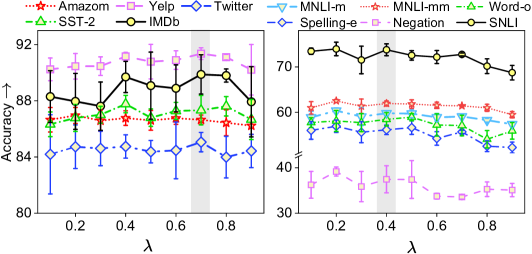
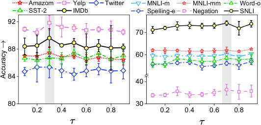
C.4 Hyperparemeter analysis: and
In this study, we investigate the influence of trade-off factor and temperature on model generalization. Specifically, we incrementally increase or from 0.1 to 0.9 by 0.1 and fix other best hyper-parameters searched from grid search. The experimental results on ID and OODs are reported in Figure 4. We observe that with or increasing from , the model performance initially increases and then declines. In SA, the model perform better for a larger and a lower temperature (i.e., ), while in NLI, a larger temperature and smaller is favored (i.e., ). We hypothesize that in SA, the model may overly depend on perturbed words for predictions, as revision patterns are relatively smaller than in NLI. Therefore, we should incorporate a smaller temperature and a higher trade-off to introduce a higher regularization from contrastive learning in SA. More insights will be explored in future work.
C.5 Few-shot learning on SA
Here, we present the results of few-shot learning using the BERT model on the SA task, with the number of IMDb augmented data progressively increasing from 32 to 1024, as shown in Figure 5. Similar to the trend observed in few-shot learning for the NLI task, discussed in Section 5.2, our approach demonstrates significant performance improvements even with limited data in the SA task.
| Sentiment Analysis | Natural Language Inference | ||||||||||
| In-Domain | Out-of-Dimain | In-Domain | Out-of-Dimain | ||||||||
| Baseline vs. Ours | IMDb | Amazon | Yelp | SST-2 | SNLI | MNLI-m | MNLI-mm | Negation | Spelling-e | Word-o | |
| BERT-base-uncased | |||||||||||
| Vanilla | 0.3237 | 0.0495 | 0.0043 | 2.40E-06 | 1.63E-05 | 0.0012 | 0.0136 | 0.0111 | 0.5754 | 0.0140 | 0.1182 |
| BTSCL | 0.0665 | 0.0411 | 0.1075 | 0.0005 | 2.11E-06 | 2.75E-05 | 0.0044 | 0.0053 | 0.1491 | 0.0101 | 0.0047 |
| CouCL | 7.72E-06 | 0.8357 | 6.10E-05 | 0.0204 | 0.0012 | 0.0005 | 0.0001 | 8.17E-05 | 0.7220 | 0.0007 | 0.0004 |
| HCAD | 0.077 | 0.1308 | 0.001 | 0.0498 | 0.002 | 0.0323 | 0.0382 | 0.0637 | 0.1826 | 0.0590 | 0.0588 |
| CFGSL | 0.3011 | 0.0457 | 0.0141 | 0.0421 | 0.5235 | 1.06E-05 | 0.0932 | 0.8232 | 0.0018 | 0.0078 | 0.0040 |
| ECF | 0.0279 | 0.0457 | 6.61E-06 | 0.0003 | 0.2573 | 0.1848 | 0.0177 | 0.0867 | 0.3704 | 0.0346 | 0.1361 |
| RoBERTa-base | |||||||||||
| Vanilla | 0.0448 | 0.046 | 0.0495 | 0.0029 | 0.0469 | 1.45E-06 | 0.0102 | 0.0715 | 0.2057 | 0.0225 | 0.0452 |
| BTSCL | 0.0394 | 0.2731 | 0.0019 | 0.0231 | 0.0266 | 6.26E-05 | 0.0484 | 0.3835 | 0.9955 | 0.0344 | 0.0076 |
| CouCL | 0.0410 | 0.1456 | 0.0462 | 0.0443 | 0.0182 | 0.0922 | 0.0584 | 0.0207 | 0.0396 | 0.1400 | 0.0376 |
| HCAD | 0.0442 | 0.0349 | 0.0154 | 0.0014 | 0.0029 | 6.51E-05 | 0.0030 | 0.0005 | 0.0008 | 0.0180 | 0.0286 |
| CFGSL | 0.0317 | 0.0241 | 0.1834 | 0.0007 | 0.0380 | 0.0348 | 0.3550 | 0.0496 | 0.0033 | 0.7874 | 0.0014 |
| ECF | 0.0361 | 0.031 | 0.0012 | 0.0012 | 0.0021 | 0.0167 | 0.0147 | 0.0112 | 0.0830 | 0.0121 | 0.0071 |
| SBERT-multi-qa-cos | |||||||||||
| Vanilla | 0.4796 | 1.56E-08 | 0.0002 | 3.66E-05 | 0.0003 | 6.48E-05 | 0.0273 | 0.0132 | 0.0076 | 0.0383 | 0.0306 |
| BTSCL | 0.0470 | 1.71E-07 | 2.01E-11 | 1.11E-07 | 4.70E-03 | 2.94E-05 | 0.0138 | 0.003 | 0.0006 | 0.04611 | 0.0035 |
| CouCL | 0.0097 | 0.0001 | 0.0002 | 0.0004 | 0.0099 | 0.0403 | 0.0448 | 0.0275 | 0.1397 | 0.0569 | 0.0428 |
| HCAD | 0.0173 | 7.43E-05 | 0.0025 | 0.0221 | 4.51E-05 | 0.0051 | 0.0584 | 0.0457 | 0.079 | 0.0422 | 0.0498 |
| CFGSL | 0.0050 | 0.0006 | 0.008 | 4.22E-06 | 0.0197 | 0.0325 | 0.0421 | 0.03106 | 0.485 | 0.0215 | 0.0533 |
| ECF | 0.0959 | 0.4188 | 0.3184 | 0.0013 | 0.3667 | 0.0008 | 0.0019 | 0.0013 | 0.1876 | 0.0019 | 0.0017 |
| T5-base | |||||||||||
| Vanilla | 0.1072 | 0.0144 | 6.37E-05 | 0.0002 | 0.0112 | 0.0216 | 0.0299 | 0.0162 | 0.0294 | 0.0302 | 0.0088 |
| BTSCL | 0.0025 | 0.0300 | 8.42E-05 | 8.42E-05 | 8.42E-05 | 0.0207 | 0.0468 | 0.0356 | 0.0349 | 0.0445 | 0.0411 |
| CouCL | 0.0464 | 0.1554 | 0.03123 | 0.019 | 0.0027 | 0.0319 | 0.0407 | 0.0459 | 0.0397 | 0.0309 | 0.0211 |
| HCAD | 0.0306 | 0.1720 | 0.0012 | 0.0028 | 0.0001 | 0.0463 | 0.0566 | 0.0772 | 0.4857 | 0.0421 | 0.0438 |
| CFGSL | 0.4158 | 0.1139 | 0.2299 | 0.0067 | 0.0014 | 0.0497 | 0.0452 | 0.0229 | 0.4665 | 0.0416 | 0.0721 |
| ECF | 0.0053 | 0.2914 | 0.0065 | 0.1045 | 0.4612 | 0.0352 | 0.0976 | 0.0452 | 0.4403 | 0.0321 | 0.0813 |
| Sentiment Analysis | Natural Language Inference | |||||||||||
|---|---|---|---|---|---|---|---|---|---|---|---|---|
| Variants | In-Domain | Out-of-Dimain | In-Domain | Out-of-Dimain | ||||||||
| Control | Comparison | IMDb | Amazon | Yelp | SST-2 | SNLI | MNLI-m | MNLI-mm | Negation | Spelling-e | Word-o | |
| BERT-base-uncased | ||||||||||||
| CE | Shuff vs. Pair | 0.8727 | 0.5053 | 0.9418 | 0.3465 | 0.4981 | 0.1934 | 0.2881 | 0.7977 | 0.4542 | 0.0450 | 0.3317 |
| CE+CL | Shuff vs. Pair | 0.0389 | 0.9057 | 0.0055 | 0.1469 | 0.0350 | 0.0120 | 0.0011 | 0.1890 | 0.0268 | 0.0008 | 0.0406 |
| ShuffCAD | CE vs. CE+CL | 0.2311 | 0.1238 | 0.0018 | 0.1890 | 0.0155 | 0.5306 | 0.1866 | 0.0973 | 0.2621 | 0.1722 | 0.0736 |
| PairCAD | CE vs. CE+CL | 0.2021 | 0.3666 | 0.0417 | 0.0395 | 0.0032 | 0.0135 | 0.0034 | 0.0137 | 0.0293 | 0.2280 | 0.0210 |
| RoBERTa-base | ||||||||||||
| CE | Shuff vs. Pair | 0.0376 | 0.0045 | 0.0049 | 0.9751 | 0.4894 | 0.0246 | 0.3194 | 0.0723 | 0.0031 | 0.2519 | 0.3029 |
| CE+CL | Shuff vs. Pair | 0.3722 | 0.1181 | 0.0720 | 0.3250 | 0.0009 | 0.2123 | 0.0037 | 0.3623 | 0.0072 | 0.0033 | 0.0007 |
| ShuffCAD | CE vs. CE+CL | 0.0005 | 2.48E-06 | 6.52E-05 | 8.76E-07 | 0.0073 | 0.0004 | 0.0178 | 0.0016 | 0.0006 | 0.0540 | 0.0655 |
| PairCAD | CE vs. CE+CL | 0.0298 | 0.0133 | 0.1017 | 0.0120 | 0.0011 | 0.1585 | 0.0012 | 0.0252 | 0.2565 | 0.0040 | 0.2420 |
| SBERT-multi-qa-distilbert-cos | ||||||||||||
| CE | Shuff vs. Pair | 0.0058 | 9.65E-09 | 0.0011 | 0.6263 | 0.0086 | 0.0491 | 0.3697 | 0.3337 | 0.2248 | 0.5029 | 0.4971 |
| CE+CL | Shuff vs. Pair | 0.1317 | 0.0004 | 0.4958 | 1.65E-07 | 0.0027 | 0.6576 | 0.6699 | 0.0187 | 0.0476 | 0.4170 | 0.1311 |
| ShuffCAD | CE vs. CE+CL | 0.0003 | 4.29E-04 | 3.43E-06 | 0.0049 | 0.0021 | 0.4285 | 0.0930 | 0.1230 | 0.5577 | 0.0494 | 0.1786 |
| PairCAD | CE vs. CE+CL | 0.1491 | 1.41E-06 | 0.6202 | 0.0002 | 0.0002 | 0.2408 | 0.1698 | 0.0011 | 0.1113 | 0.0335 | 0.0118 |
| T5-base | ||||||||||||
| CE | Shuff vs. Pair | 0.8304 | 0.1841 | 0.1112 | 0.0013 | 0.0006 | 0.0024 | 2.99E-06 | 0.0006 | 0.9644 | 0.0003 | 0.0002 |
| CE+CL | Shuff vs. Pair | 0.0029 | 0.1851 | 0.0096 | 0.0108 | 0.0004 | 0.2966 | 0.0042 | 0.0415 | 0.5030 | 0.1371 | 0.1530 |
| ShuffCAD | CE vs. CE+CL | 0.4340 | 0.1206 | 0.0876 | 0.4625 | 0.0164 | 0.5484 | 0.4942 | 0.4354 | 0.4859 | 0.4489 | 0.2817 |
| PairCAD | CE vs. CE+CL | 0.0029 | 0.1837 | 0.0096 | 0.0108 | 0.0004 | 0.0481 | 0.0098 | 0.0223 | 0.4851 | 0.0284 | 0.0497 |
C.6 Statistical significance test
To ensure that the observed improvements are not due to randomness across multiple trials, we conducted statistical significance tests on comparative experiments and ablation studies. We first check that experimental results from random initialization on both ID and OOD datasets follow a Gaussian distribution, and thus employ a two-sided paired samples T-test. Our T-tests are conducted under the null hypothesis that there are no differences between the two groups of experiments.
Table 11 presents the significance test results of our method against all baselines for the comparative experiments (refer to Table 1). We observed that the majority of p-values fall below the conventional confidence level of 0.05, indicating that the improvements in OOD performance achieved by our algorithm over the baselines are statistically significant and not due to randomness. Similarly, Table 11 presents the significance test results of the ablation study (refer to Table 2), verifying the effectiveness of our pairing strategy and CL function.