Pairing by a dynamical interaction in a metal
Abstract
We consider pairing of itinerant fermions in a metal near a quantum-critical point (QCP) towards some form of particle-hole order (nematic, spin-density-wave, charge-density-wave, etc). At a QCP, the dominant interaction between fermions comes from exchanging massless fluctuations of a critical order parameter. At low energies, this physics can be described by an effective model with the dynamical electron-electron interaction , up to some upper cutoff . The case corresponds to BCS theory, and can be solved by summing up geometric series of Cooper logarithms. We show that for a finite , the pairing problem is still marginal (i.e., perturbation series are logarithmic), but one needs to go beyond logarithmic approximation to find the pairing instability. We discuss specifics of the pairing at in some detail and also analyze the marginal case , when . We show that in this case the summation of Cooper logarithms does yield the pairing instability at , but the logarithmic series are not geometrical. We reformulate the pairing problem in terms of a renormalization group (RG) flow of the coupling, and show that the RG equation is different in the cases , , and .
I Preface
It is our great pleasure to present this paper for the special issue of JETP devoted to 90th birthday of Igor Ekhielevich Dzyaloshinskii. His works on correlated electron systems are of highest scientific quality. He made seminal contributions to quantum magnetism, superconductivity, Fermi-liquid theory, and to other subfields of modern condensed matter physics. In a number of works, including the famous ones on the interplay between d-wave superconductivity and antiferromagnetism at the beginning of “high - era” (Refs. Zheleznyak et al. (1997); Dzyaloshinskii (1987); Dzyaloshinskii and Yakovenko (1988)), Igor Ekhielevich used the renormalization group technique to obtain the flow of the couplings upon integrating out fermions with higher energies. In this study, we apply the same RG technique to analyze the pairing instability in systems with critical dynamical pairing interaction. We consider this as a natural extension of his works. Happy birthday, Igor Ekhielevich, and the very best wishes.
II Introduction.
The pairing near a quantum-critical point (QCP) in a metal and its interplay with non-Fermi-liquid behavior in the normal state, is a fascinating subject, which attracted substantial attention in the correlated electron community after the discovery of superconductivity (SC) in the cuprates, Fe-based systems, heavy-fermion materials, organic materials, and, most recently, twisted bilayer graphene Monthoux et al. (2007); Scalapino (2012); Norman (2014); Maiti and Chubukov (2014); Keimer et al. (2015); Shibauchi et al. (2014); Fernandes and Chubukov (2016); Fradkin et al. (2010); Yang et al. (2006); Fratino et al. (2016); Sachdev (2018); Coleman (2015); Cao et al. (2018). Itinerant QC models, analyzed in recent years, include models of fermions in spatial dimensions , various two-dimensional models near zero-momentum spin and charge nematic instabilities, and instabilities towards spin and charge density-wave order with either real or imaginary (current) order parameter, 2D fermions at a half-filled Landau level, Sachdev-Ye-Kitaev (SYK) and SYK-Yukawa models, strong coupling limit of electron-phonon superconductivity, and even color superconductivity of quarks, mediated by gluon exchange. These problems have also been studied analytically and using various numerical techniques. We refer a reader to Ref. Abanov and Chubukov (2020), where the extensive list of references to these works has been presented.
From theory perspective, pairing near a QCP is a fundamentally novel phenomenon because an effective dynamic electron-electron interaction, , mediated by a critical collective boson, which condenses at a QCP, provides a strong attraction in one or more pairing channels and, at the same time, gives rise to a non-Fermi liquid (NFL) behavior in the normal state. The two tendencies compete with each other: fermionic incoherence, associated with the NFL behavior, destroys the Cooper logarithm and reduces the tendency to pairing, while an opening of a SC gap eliminates the scattering at low energies and reduces the tendency to a NFL. To find the winner of this competition (SC or NFL), one needs to analyze the set of integral equations for the fermionic self-energy, , and the gap function, , for fermions with momentum/frequency and .
We consider the subset of models, in which collective bosons are slow modes compared to dressed fermions, for one reason or the other. In this situation, which bears parallels with Eliashberg theory for electron-phonon interaction Eliashberg (1960), the self-energy and the pairing vertex can be approximated by their values on the Fermi surface (FS) and computed within the one-loop approximation. The self-energy on the FS, , is invariant under rotations from the point group of the underlying lattice. The rotational symmetry of the gap function and the relation between the phases of on different FS’s in multi-band systems are model specific. E.g., near an antiferromagnetic QCP in a system with a single FS, the strongest attraction is in the wave channel. In each particular case, one has to project the pairing interaction into the irreducible channels, find the strongest one, and solve for the pairing vertex for a given pairing symmetry.
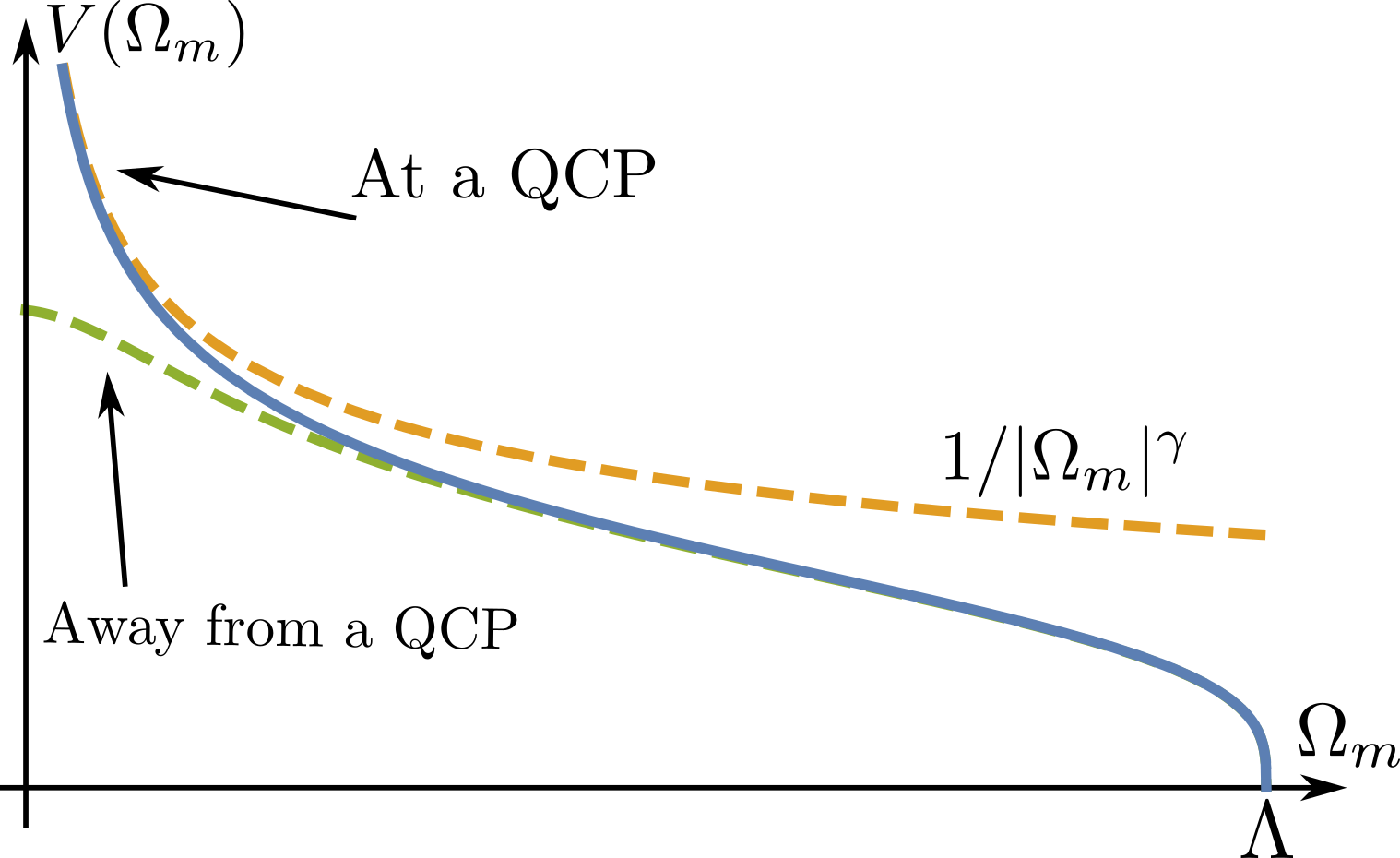
Away from a QCP, the effective tends to a finite value at . In this situation, the fermionic self-energy has a FL form at the smallest frequencies, and the equation for is similar to that in a conventional Eliashberg theory for phonon-mediated superconductivity; the only qualitative distinction for electronically-mediated pairing is that by itself changes below due to feedback from fermionic pairing on collective modes. At a QCP, the situation is qualitatively different because the effective interaction , mediated by a critical massless boson, is a singular function of frequency. Quite generally, such interaction behaves at the smallest on the Matsubara axis as , where is some exponent. (Fig. 1). This holds at frequencies below some upper cutoff . At larger , the interaction drops even further, and can be safely neglected.
In these notations, BCS pairing corresponds to . The superconducting transition temperature inthe BCS case can be most straightforwardly obtained by computing the pairing susceptibility in the order-by-order expansion in the coupling and identifying the temperature at which it diverges. The series contain the powers of the product of the Cooper logarithm and the dimensionless coupling , defined such that is the ratio of the renormalized and the bare electron masses. The series are geometrical, i.e., . We will see that for , the pairing kernel still has a marginal form, and, as a result, the series for still contain logarithms. However, contrary to the BCS case, where comes from the fermionic propagator, the marginal exponent for is the sum of the exponent from the interaction and from the fermionic self-energy (see below). As a result, the logarithmic series are not geometric, and we will see that does not diverge down to . We show that the pairing instability still exists, however one needs to go beyond the logarithmic approximation to obtain it.
We show that there exists a special case, which falls in between and . This is the limit , when . In this limit, the pairing instability still can be detected by summing up the series of logarithms for . However, the series are not geometric, and some extra efforts are needed to sum them up to find the form of and detect the pairing instability at .
The model with the interaction displays a very rich physics, and our group has studied it over the last few years. This physics is particularly interesting for , where a wide range of the pseudogap (preformed pair) behavior emerges, and for , when the new, non-superconducting ground state emerges Wu et al. (2020a). In this communication, we will not discuss these values of but instead focus on small and discuss in some detail the difference between BCS pairing at and the pairing at and at . We derive the Eliashberg equation for the pairing vertex and analyze it within logarithmic perturbation theory and beyond it. We then convert the integral Eliashberg equation into the approximate differential equation and obtain and solve the corresponding renormalization group (RG) equation.
The pairing problem at small attracted a lot of attention in the last few years from various physics sub-communities of physicists Mross et al. (2010); Metlitski et al. (2015); Raghu et al. (2015); Mahajan et al. (2013); *raghu2; *raghu3; *raghu4; *raghu5; Wang et al. (2017, 2018); Fitzpatrick et al. (2015b); Wang and Chubukov (2013); Wu et al. (2019a); Son (1999); Chubukov and Schmalian (2005); Schäfer and Wilczek (1999); Pisarski and Rischke (2000); Wang and Rischke (2002); Damia et al. (2020) . The pairing interaction with emerges for fermions near a generic particle-hole instability in a weakly anisotropic 3D system (more explicitly, in dimension , where , Refs. Mross et al. (2010); Metlitski et al. (2015); Raghu et al. (2015) ). A similar gap equation with small holds for the pairing in graphene Khveshchenko (2009). The model with describes the pairing in 3D systems and color superconductivity of quarks due to gluon exchange Son (1999); Schäfer and Wilczek (1999); Pisarski and Rischke (2000); Wang and Rischke (2002). The model yields a marginal Fermi liquid form of the fermionic self-energy in the normal state and was argued Varma et al. (1989); *Littlewood_92; Varma (2020) to be relevant to pairing in the cuprates and, possibly, in Fe-based superconductors.
The structure of the paper is at follows. In the next Section we present the set of coupled Eliashberg equations for the pairing vertex and the fermionic self-energy and combine them into the equation for the gap function . In Sec. IV we analyze the structure of the logarithmic perturbation theory for and . In Sec. V we go beyond perturbation theory and re-express the integral Eliashberg equation as an approximate differential equation for the pairing vertex and solve it. We show that for , the solution coincides with the result of summation of logarithmic series. For , we show that the system does become unstable towards pairing if the interaction exceeds a certain threshold. In Sec. VI we analyze the pairing at small from RG perspective and reproduce the results of the previous Section. We present our conclusions in Sec. VII.
III The model
We consider itinerant fermions at the onset of a long-range particle-hole order in either spin or charge channel. At a critical point, the propagator of a soft boson becomes massless and mediates singular interaction between fermions. A series of earlier works on spin-density-wave order, charge-density-wave order, Ising-nematic order, etc (see Ref.Abanov and Chubukov (2020) for references) have found that this interaction is attractive in at least one pairing channel. We take this as in input and project boson-mediated interaction into the channel with the strongest attraction. As we said, at small frequencies, the interaction scales as . We incorporate dimension-full factors, like the density of states, into and treat it as dimensionless. We assume that the power-law form holds up to the scale , and set above this scale. To keep continuous at and also to transform gradually between and , we use the following form for (Fig.1):
| (1) |
Here is a dimensionless coupling, and has units of energy. We assume that , but the ratio can be arbitrary. At , the last term in (1) can be expanded in and yields the logarithmic interaction
| (2) |
The conventional BCS/Eliashberg case in this notations is obtained by extending (1) to the case when a pairing boson has a finite mass. In this situation, is replaced by a constant below a certain scale. In BCS theory, this scale is assumed to be comparable to , such that up to , and zero at larger .
Below we measure all quantities with the dimension of energy, i.e., , in units of , i.e., introduce , and . Throughout this paper we assume that .
Earlier works on the pairing mediated by a soft collective boson found that a boson is overdamped due to Landau damping into a particle-hole pair and can be treated as slow mode compared to a fermion, i.e., at the same momentum , a typical fermionic frequency is much larger than a typical bosonic frequency. This is the same property that justified Eliashberg theory of phonon-mediated superconductivity. By analogy, the theory of electronic superconductivity, mediated by soft collective bosonic excitations in spin or charge channel, is often referred to as Eliashberg theory, and we will be using this convention.
In Eliashberg theory, one can explicitly integrate first over the momentum component perpendicular to the Fermi surface and then over the component(s) along the Fermi surface, and reduce the pairing problem to a set of coupled integral equations for frequency dependent self-energy and the pairing vertex .
At , the coupled Eliashberg equations are
| (3) |
where . In these equations, both and are real functions. Observe that we define with the overall plus sign and without the overall factor of . In the normal state (), we have at , and
| (4) |
At ,
| (5) |
The superconducting gap function is defined as the ratio
| (6) |
The equation for is readily obtained from (III):
| (7) |
This equation contains a single function , but for the cost that appears also in the r.h.s., which makes Eq. (7) less convenient for the analysis than Eqs. (III).
For a generic , the coupled equations (III) for and describe the interplay between the two competing tendencies – one towards superconductivity, specified by , and the other towards incoherent NFL normal-state behavior, specified by . The competition between the two tendencies is encoded in the fact that appears in the denominator of the equation for and appears in the denominator of the equation for . In more physical terms, a self-energy is an obstacle to Cooper pairing, while when is non-zero, it reduces the strength of the self-energy and renders fermionic coherence.
The full set of the equations for electron-mediated pairing generally must contain the third equation, describing the feedback from the pairing on the bosonic propagator. This feedback is small in the case of electron-phonon interaction, but is generally not small when the pairing is mediated by a collective mode because the dispersion of a collective mode changes qualitatively below (Refs. Abanov et al. (2003, 2001a)). In this work, we only consider the computation of and will not discuss system behavior below . For this computation, it is sufficient to restrict with the two equations (III). Moreover, we can (i) treat as infinitesimally small and neglect it in the denominator of Eq. (III), and (ii) use Eqs. (4) or (5) for . For a small, but finite , the linearized equation for the pairing vertex is
| (8) |
Observe that the overall coupling is just a number, equal to one, because the factor in cancels out with the same factor in the self-energy. This factor is still present in the denominator, but in the term, which contains and becomes irrelevant at the smallest frequencies
At , the linearized equation for is
| (9) |
IV Summing up the logarithms
As a first try, we analyze the linearized equation for the pairing vertex perturbatively, by adding up a trial, infinitesimally small to the r.h.s of Eqs. (8) and (9) and computing the pairing susceptibility perturbatively, order-by-order. Such approach has been commonly used for BCS pairing. The perturbation series there contain singular Cooper logarithms. The logarithmic singularity can be cut either by a finite or at , by a finite total incoming bosonic frequency, . For consistency with other cases, we set and keep finite. The result of order-by-order analysis for a BCS pairing is well known:
| (10) |
The ratio (the pairing susceptibility) diverges at and becomes negative at smaller , indicating that the normal state is unstable towards pairing. (In a more accurate description, the pole in moves from the lower to the upper half-plane of complex frequency Abrikosov et al. (1965)).
We now do the same calculation for . The kernel in Eq. (8) is still marginal at , but, as we said, now the scaling dimension is the sum of , coming from the interaction, and , coming from the self-energy. This implies that perturbation theory still contains logarithms, but in distinction to BCS, each logarithmical integral runs between the upper cutoff at and the lower cutoff at . Because the lower cutoff is finite, we can set . Summing up the logarithmical series, we then obtain Abanov et al. (2001b)
| (11) |
We see that the pairing susceptibility increases as decreases, but remains finite and positive for all finite , even when . Re-doing calculations at a finite we find the same result as in (11), with replaced by max. This implies that for , there is no signature of a pairing instability within the logarithmic approximation. The absence of a pairing instability within the logarithmic approximation generally implies that pairing does not develop at weak coupling and, if exists, is a threshold phenomenon. In our case, the dimensionless coupling in the series in Eq. (11) is a number equal to one, i.e., the problem we consider is not weak-coupling. A weak-coupling limit can be reached if we extend the model and make the pairing interaction parametrically smaller than the one in the particle-hole channel. In practice, this is done by multiplying the interaction in the pairing channel by , where (Refs. Raghu et al. (2015); Wang et al. (2016); Abanov et al. (2019); *Wu_19_1; Abanov and Chubukov (2020); Damia et al. (2020)), while the interaction in the particle-hole channel is left intact 111The extension to was originally rationalized by extending the original model to matrix , with integer , hence the notation. We treat as a continuous parameter. In the extended model, gets multiplied by , and at large the problem becomes weak-coupling. We show below that indeed there is no pairing instability at large .
The case falls in between BCS and cases. Namely, we show below that the series of logarithms are not geometric, like the ones for , however by summing up the series one does find the scale of a pairing instability, like in BCS. We assume and than verify that for relevant , is small for , and neglect this term in the denominator of (9). We keep non-zero to avoid divergencies and for simplicity set and to be comparable. To logarithmic accuracy, we can then view as a function of a single parameter .
Because the interaction is logarithmic, perturbation series hold in . Evaluating the pairing vertex in order-by-order calculations, we find (see Appendix for details)
| (12) |
At a first glance, the coefficients in (12) are just some uncorrelated numbers. On a more careful look, we realize that the series fall into
| (13) |
Accordingly, the pairing susceptibility diverges when the argument of becomes , i.e., at . It is natural to associate this scale with (Ref. Son (1999)). The susceptibility also diverges at a set of smaller , but here we focus only on the highest onset temperature. We see that has exponential dependence on the coupling, like in BCS theory, however the argument of the exponent contains rather than . This in turn justifies the neglect of the self-energy, because for relevant frequencies, (the corrections due to self-energy have been analyzed in Ref. Wang and Rischke (2002)).
To summarize, the case is similar to BCS in the sense that pairing occurs for arbitrary weak coupling ( remains finite even if we replace by and set to be large). However, for and finite , there is no indication of the pairing instability within the logarithmic approximation.
V The differential equation for
We now analyze the linearized equation for the pairing vertex for beyond the logarithmic approximation. To do this, we convert integral equation (8) into to a differential equation with certain boundary conditions and solve it non-perturbatively.
V.1 The case
We first consider the case . We keep as a parameter, as we need to verify our earlier conjecture that there is no pairing instability for large enough . To convert (8) into differential equation, we use the fact that at small , the integral in the r.h.s. of (8) predominantly comes from internal , which are either substantially larger or substantially smaller than the external . We then split the integral over into two parts: in one we approximate by , in the other by . Introducing , we then simplify (8) to
| (14) |
where (). Differentiating this equation twice over and replacing by , we obtain the second order differential gap equation in the form (Refs. Wang et al. (2017, 2018, 2016); Abanov and Chubukov (2020))
| (15) |
where and
| (16) |
This has to be real and satisfy the boundary conditions at large and at . At large , we expect perturbation theory to work, hence . The boundary condition at is set by the requirement that is normalizable, i.e., that the ground state energy for a non-zero must be free from divergencies. This requirement imposes the condition that should be infra-red convergent (Refs. Abanov and Chubukov (2020); Yuzbashyan et al. ).
The solution of (15) is expressed via a Hypergeometric function, and the form of depends on whether is real or imaginary, i.e., whether is larger or smaller than . When , is real, and the solution is
| (17) |
where
| (18) |
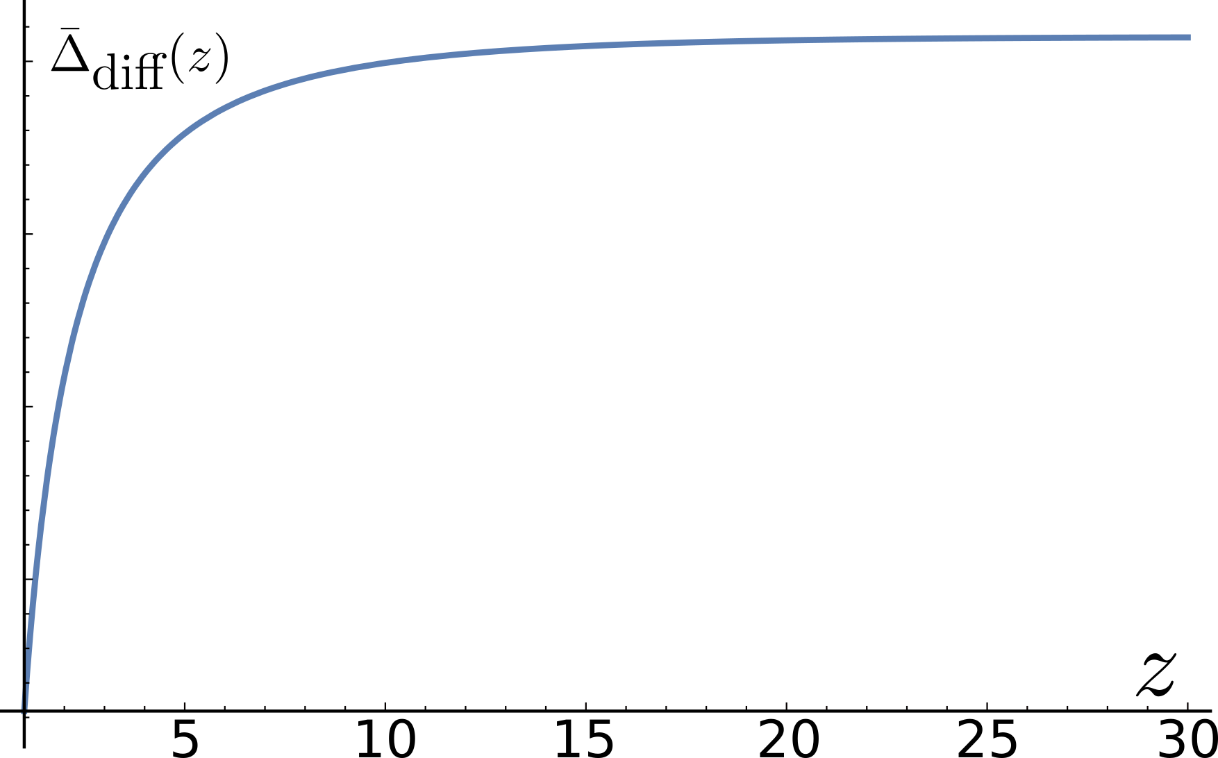
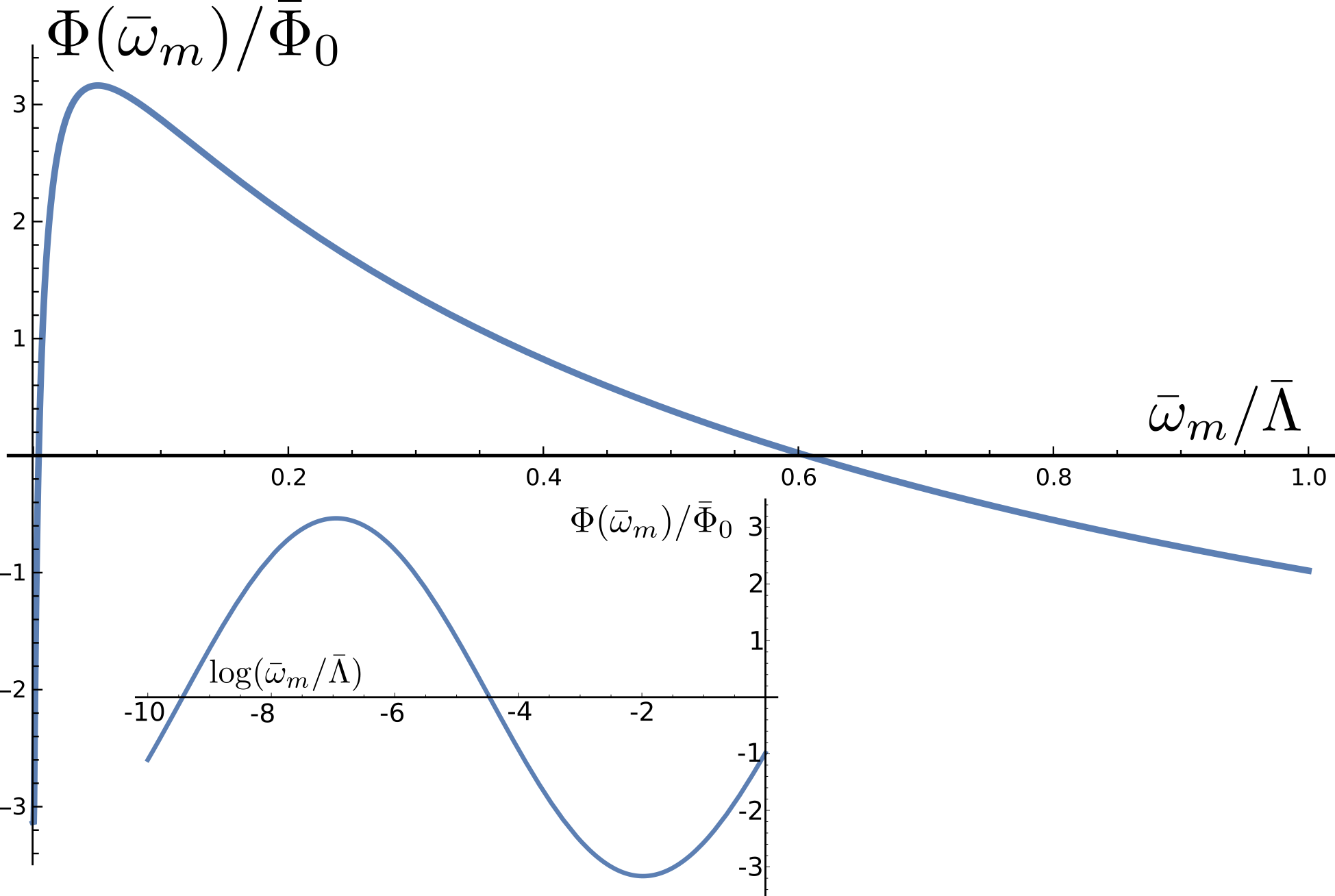
Both and are sign-preserving functions. At small , , and at large , tend to finite values . The boundary condition at sets , and the one at sets the linear relation between and . We plot for and in Fig. 2. We see that remains positive for all , i.e., the normal state remains stable with respect to pairing. At , , and . This is the same result that we obtained by summing up the logarithms. We see that in this parameter range the non-logarithmic terms just change the exponent from to .
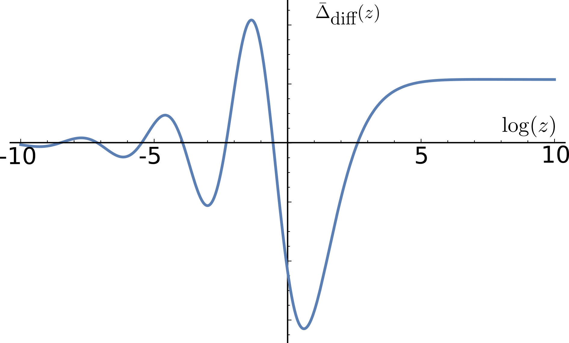
This behavior holds as long as is real, i.e., . For models with smaller , including our original model with , is imaginary, , were . In this situation, the solution of the differential equation is
| (19) |
The boundary condition at is satisfied as at small , acquires a form of a free quantum particle with a ”coordinate” . At , tends to a constant for a generic , and the boundary condition sets up a linear relation between and .
We plot in Fig. (2). We see that the gap function now passes through a minimum at some and oscillates at smaller . The oscillating behavior at could not be obtained within perturbation theory starting from as the kernel in Eq. (8) is entirely positive. This strongly suggests that the normal state is now unstable towards pairing, and sets the value of . To verify this, in Ref. Wu et al. (2020b) we solved the gap equation at a finite . This calculation is a bit more tricky due to special behavior of fermions with Matsubara frequencies , but nevertheless it confirms the two key points of our analysis that superconducting is finite and is generally of order .
Note that the value of depends on the magnitude of , i.e., on the ratio . For small , which holds when is only slightly below , the first sign change of occurs at small , where . For larger , the first sign change occurs at , i.e., at , or, equivalently, at . This holds for the original model with .
We note in passing that contains two parameters: the overall factor and the phase factor . The boundary condition at then still leaves the freedom of, e.g., choosing for a given . This extra freedom comes about because it turns out Abanov and Chubukov (2020) that the homogeneous gap equation (the one without ) by itself has a non-zero solution at , such that is the sum of the induced and the homogeneous solutions of (8). To demonstrate this more explicitly, we set , use the fact that in this range a hypergeometric function reduces to a combination of Bessel and Neumann functions, and re-express (19) as
| (20) |
where and are Bessel and Neumann functions, respectively. At small value of the argument, and , i.e., the first term vanishes at large , while the second one tends to a constant. Then is uniquely determined by the boundary condition set by , while the piece is the solution of the equation without .
The existence of the solution of the linearized gap equation at (well below ) is a highly non-trivial feature of pairing at a QCP, that affects fluctuation corrections to superconducting order parameter. For our purposes, however, we only need to analyze only the induced solution to get an estimate of . We can set in (20) and determine from the boundary condition at .
V.2 The case of a finite
At this stage, we have two different energy scales, which we identified with . Namely, at a finite and , we found . At and finite , we found . We now analyze the crossover between the two energies. For definiteness, we consider the original model with .
We argued earlier that for the pairing at , fermions can be treated as free quasiparticles, because for relevant fermions the ratio . The same holds for the case and . Here, the ratio , and for , . We now use this simplification and re-analyze the differential equation for at a finite .
One can verify that the differential equation retains the same for as for :
| (21) |
and its solution is still a linear combination of Bessel and Neumann functions, Eq. (20). However, we have an extra requirement
| (22) |
where . There is no solution of the homogeneous equation at a finite , and Eq. (22) together with the boundary condition uniquely specify the coefficients and in (20):
| (23) |
where . It is convenient to introduce a dimensionless parameter
| (24) |
In the left panel of Fig. 3 we plot for a representative . We see that the gap function is regular at , but passes through an extremum and oscillates at smaller . The position of the first extremum depends on . We now show that the two forms of , which we found earlier, correspond to the limits and .
When , one can use the forms of Bessel and Neumann functions at large argument,
| (25) |
and obtain
| (26) |
In the original variables and , this reduces, to the leading order in , to
| (27) |
Associating with the position of the first extremum of , we find . This coincides with the estimate of from the analysis of the pairing susceptibility as a function of the total frequency of two fermions in a pair (see Eq. (13)).
In the opposite limit , we use and and keep only . We then obtain from (23) that the dependence on appears only in the overall factor:
| (28) |
or, in terms of ,
| (29) |
The first extremum is now located at , i.e., . This agrees with the analysis at .
In the right panel in Fig. 3 we sketch the evolution of as a function of . In terms of , scales as for (the limit of large and finite ), and saturates at for (the limit and finite ). The crossover between the two regimes occurs at .
We note in passing that Eq. (27) could also be obtained directly, by converting the gap equation for into the differential equation Chubukov and Schmalian (2005). For this we depart from Eq. (9), neglect the self-energy term in the denominator, split the integral over into contributions from and , as we did in the derivation of (14), and introduce logarithmic variables , . We then obtain
| (30) |
Differentiating twice over and introducing , we obtain
| (31) |
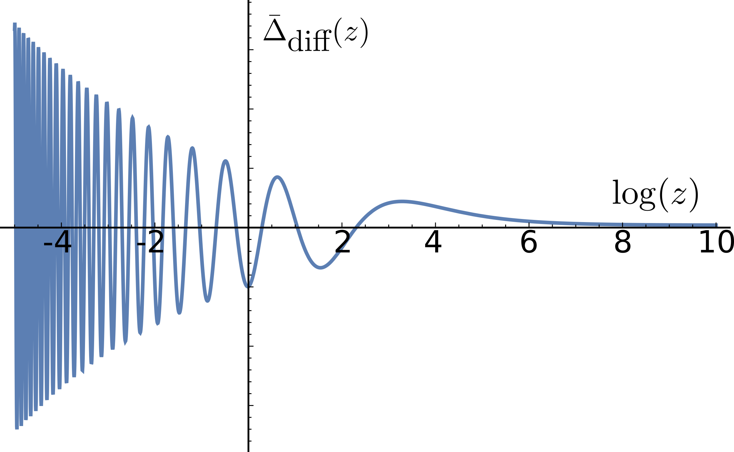
This equation is valid only for , and the two boundary conditions are and . The solution of (31), which satisfies the boundary conditions, is, for small ,
| (32) |
In the original units, this becomes
| (33) |
We plot in Fig. 4. We see that is sign-preserving when is small, but oscillates when gets larger. Associating the position of the first extremum of with , as we did before, we find the same as at in our earlier treatment.
VI RG analysis
The difference between and at a finite can be also understood by analyzing the flow of the running 4-fermion pairing vertex within the RG formalism. The RG equations for small have been derived in Refs. Metlitski et al. (2015); Wang et al. (2017) and for in Ref. Son (1999) (see also Refs. Schäfer and Wilczek (1999); Pisarski and Rischke (2000)).
The key point for the RG analysis is that at small but finite , the interaction in (1) can be approximated by
| (34) |
and both the logarithmic and the power-law dependence have to be kept. This interaction can be further re-expressed in terms of as the product of and the running effective , where .
The interaction acts as the source for the running 4-fermion pairing vertex, which we label as . Without the source, would obey a BCS RG equation . With the source, the equation becomes
| (35) |
The solution of this equation, subject to (no pairing without the source), is Metlitski et al. (2015); Wang et al. (2017)
| (36) |
For , relevant values of the arguments of Bessel and Neumann functions are large, and using using their asymptotic forms, Eq. (25), we find that, to leading order in ,
| (37) |
The 4-fermion vertex diverges at the same that we obtained before.
In the opposite limit , we use that . Keeping only in (36), we obtain
| (38) |
The 4-fermion vertex now diverges at the first zero of , i.e., at
| (39) |
Solving for , we obtain . This agrees the result of our earlier analysis of the case and .
VII Conclusions
The goal of this work was to analyze the crossover from a conventional BCS pairing by a massive boson to a pairing at a quantum-critical point towards some particle-hole order, when the pairing boson becomes massless. We considered a subset of quantum-critical models, in which the pairing boson is a slow mode compared to fermions, and an effective low-energy theory is purely dynamical, with an effective dynamical interaction , up to some upper cutoff . The case corresponds to BCS theory od pairing from a Fermi liquid. We considered the pairing at a small, but finite , when the normal state is a NFL, and the case , when , and the normal state is marginal Fermi liquid. We demonstrated that for , the pairing instability can still be detected by summing up series of Cooper logarithms, but for a finite one needs to go beyond the leading logarithmic approximation to analyze the pairing. We argued that in this last case, the pairing occurs only if the interaction exceeds some finite threshold. We approximated the original integer gap equation by the differential one and solved it. This allowed us to identify the threshold at and the frequency scale, associated with superconductivity, once the interaction exceeds the threshold, We found the crossover between the pairing at a finite and at and identified the parameter responsible for the crossover. We obtained the same crossover by analyzing the non-BCS RG equation for the running 4-fermion pairing vertex.
Acknowledgements.
We thank B. Altshuler, A. Finkelstein, S. Karchu, S. Kivelson, I. Mazin, M. Metlitski, V. Pokrovsky, S. Raghu, S. Sachdev, T. Senthil, J. Schmalian, D. Son, G. Torroba, E. Yuzbashyan, C. Varma, Y. Wang, Y. Wu, and S-S Zhang for useful discussions. The work by AVC was supported by the NSF DMR-1834856. AVC acknowledges the hospitality of KITP at UCSB, where part of the work has been conducted. The research at KITP is supported by the National Science Foundation under Grant No. NSF PHY-1748958.Appendix A Derivation of Eq. (12)

In this Appendix we present some details of the derivation of order-by-order logarithmic renormalization of the pairing vertex for the case . The Eliashberg equation for is Eq. (9). Adding a constant to the r.h.s. and expanding in powers of the coupling , we obtain the series in , where, we remind, in the upper cutoff, and all quantities are in units of our base energy . As we discussed in the main text, fermionic self-energy (the log term in the denominator of (9)) is small at relevant and can be safely neglected.
We show the calculations at one-loop and two-loop order. The corresponding renormalizations are graphically presented in Fig. 5. In this Figure, the two-fermion vertex is , the wavy line is , and we set both external frequencies to be . The one-loop result is obtained by integrating over a single internal frequency and is
| (40) |
At two-loop order we have to integrate over two internal frequencies and . We introduce , and use the fact that the leading logarithm comes from . Taking this limit, we obtain the two-loop correction to in the form
| (41) |
A simple analysis shows that the highest power of comes from the ranges and . Evaluating the contributions from these regions, we obtain
| (42) |
Collecting all contributions, we obtain for the two-loop renormalization
| (43) |
This leads to Eq. (12) in the main text.
References
- Zheleznyak et al. (1997) A. T. Zheleznyak, V. M. Yakovenko, and I. E. Dzyaloshinskii, Phys. Rev. B 55, 3200 (1997).
- Dzyaloshinskii (1987) I. E. Dzyaloshinskii, Sov. Phys. JETP 66, 848 (1987).
- Dzyaloshinskii and Yakovenko (1988) I. E. Dzyaloshinskii and V. M. Yakovenko, International Journal of Modern Physics B 02, 667 (1988), https://doi.org/10.1142/S0217979288000494 .
- Monthoux et al. (2007) P. Monthoux, D. Pines, and G. G. Lonzarich, Nature 450, 1177 (2007).
- Scalapino (2012) D. J. Scalapino, Rev. Mod. Phys. 84, 1383 (2012).
- Norman (2014) M. R. Norman, “Novel superfluids,” (Oxford University Press, 2014) Chap. Unconventional superconductivity.
- Maiti and Chubukov (2014) S. Maiti and A. V. Chubukov, “Novel superfluids,” (Oxford University Press, 2014) Chap. Superconductivity from repulsive interaction.
- Keimer et al. (2015) B. Keimer, S. A. Kivelson, M. R. Norman, S. Uchida, and J. Zaanen, Nature 518, 179 (2015).
- Shibauchi et al. (2014) T. Shibauchi, A. Carrington, and Y. Matsuda, Annual Review of Condensed Matter Physics 5, 113 (2014).
- Fernandes and Chubukov (2016) R. M. Fernandes and A. V. Chubukov, Reports on Progress in Physics 80, 014503 (2016).
- Fradkin et al. (2010) E. Fradkin, S. A. Kivelson, M. J. Lawler, J. P. Eisenstein, and A. P. Mackenzie, Annual Review of Condensed Matter Physics 1, 153 (2010).
- Yang et al. (2006) K.-Y. Yang, T. M. Rice, and F.-C. Zhang, Phys. Rev. B 73, 174501 (2006).
- Fratino et al. (2016) L. Fratino, P. Sémon, G. Sordi, and A.-M. S. Tremblay, Scientific Reports 6, 22715 (2016).
- Sachdev (2018) S. Sachdev, Reports on Progress in Physics 82, 014001 (2018).
- Coleman (2015) P. Coleman, Introduction to Many-Body Physics (Cambridge University Press, 2015).
- Cao et al. (2018) Y. Cao, V. Fatemi, S. Fang, K. Watanabe, T. Taniguchi, E. Kaxiras, and P. Jarillo-Herrero, Nature 556, 43 (2018).
- Abanov and Chubukov (2020) A. Abanov and A. V. Chubukov, Phys. Rev. B 102, 024524 (2020).
- Eliashberg (1960) G. M. Eliashberg, JETP 11, 696 (1960), [ZhETF, 38, 966, (1960)].
- Wu et al. (2020a) Y.-M. Wu, A. Abanov, and A. V. Chubukov, “Interplay between superconductivity and non-fermi liquid at a quantum-critical point in a metal. iv: The model and its phase diagram at ,” (2020a), arXiv:2009.10911 [cond-mat.supr-con] .
- Mross et al. (2010) D. F. Mross, J. McGreevy, H. Liu, and T. Senthil, Phys. Rev. B 82, 045121 (2010).
- Metlitski et al. (2015) M. A. Metlitski, D. F. Mross, S. Sachdev, and T. Senthil, Phys. Rev. B 91, 115111 (2015).
- Raghu et al. (2015) S. Raghu, G. Torroba, and H. Wang, Phys. Rev. B 92, 205104 (2015).
- Mahajan et al. (2013) R. Mahajan, D. M. Ramirez, S. Kachru, and S. Raghu, Phys. Rev. B 88, 115116 (2013).
- Fitzpatrick et al. (2013) A. L. Fitzpatrick, S. Kachru, J. Kaplan, and S. Raghu, Phys. Rev. B 88, 125116 (2013).
- Fitzpatrick et al. (2014) A. L. Fitzpatrick, S. Kachru, J. Kaplan, and S. Raghu, Phys. Rev. B 89, 165114 (2014).
- Torroba and Wang (2014) G. Torroba and H. Wang, Phys. Rev. B 90, 165144 (2014).
- Fitzpatrick et al. (2015a) A. L. Fitzpatrick, G. Torroba, and H. Wang, Phys. Rev. B 91, 195135 (2015a), and references therein.
- Wang et al. (2017) H. Wang, S. Raghu, and G. Torroba, Phys. Rev. B 95, 165137 (2017).
- Wang et al. (2018) H. Wang, Y. Wang, and G. Torroba, Phys. Rev. B 97, 054502 (2018).
- Fitzpatrick et al. (2015b) A. L. Fitzpatrick, S. Kachru, J. Kaplan, S. Raghu, G. Torroba, and H. Wang, Phys. Rev. B 92, 045118 (2015b).
- Wang and Chubukov (2013) Y. Wang and A. V. Chubukov, Phys. Rev. Lett. 110, 127001 (2013).
- Wu et al. (2019a) Y.-M. Wu, A. Abanov, and A. V. Chubukov, Phys. Rev. B 99, 014502 (2019a).
- Son (1999) D. T. Son, Phys. Rev. D 59, 094019 (1999).
- Chubukov and Schmalian (2005) A. V. Chubukov and J. Schmalian, Phys. Rev. B 72, 174520 (2005).
- Schäfer and Wilczek (1999) T. Schäfer and F. Wilczek, Phys. Rev. D 60, 114033 (1999).
- Pisarski and Rischke (2000) R. D. Pisarski and D. H. Rischke, Phys. Rev. D 61, 051501 (2000).
- Wang and Rischke (2002) Q. Wang and D. H. Rischke, Phys. Rev. D 65, 054005 (2002).
- Damia et al. (2020) J. A. Damia, M. Solís, and G. Torroba, Phys. Rev. B 102, 045147 (2020).
- Khveshchenko (2009) D. V. Khveshchenko, Journal of Physics: Condensed Matter 21, 075303 (2009).
- Varma et al. (1989) C. M. Varma, P. B. Littlewood, S. Schmitt-Rink, E. Abrahams, and A. E. Ruckenstein, Phys. Rev. Lett. 63, 1996 (1989).
- Littlewood and Varma (1992) P. B. Littlewood and C. M. Varma, Phys. Rev. B 46, 405 (1992).
- Varma (2020) C. M. Varma, Rev. Mod. Phys. 92, 031001 (2020).
- Abanov et al. (2003) A. Abanov, A. V. Chubukov, and J. Schmalian, Advances in Physics 52, 119 (2003).
- Abanov et al. (2001a) A. Abanov, A. V. Chubukov, and J. Schmalian, Journal of Electron spectroscopy and related phenomena 117, 129 (2001a).
- Abrikosov et al. (1965) A. A. Abrikosov, L. P. Gorkov, and I. E. Dzyaloshinski, Methods of Quantum Feld Theory in Statistical Physics (Pergamon Oxford, 1965).
- Abanov et al. (2001b) A. Abanov, A. V. Chubukov, and A. M. Finkel’stein, EPL (Europhysics Letters) 54, 488 (2001b).
- Wang et al. (2016) Y. Wang, A. Abanov, B. L. Altshuler, E. A. Yuzbashyan, and A. V. Chubukov, Phys. Rev. Lett. 117, 157001 (2016).
- Abanov et al. (2019) A. Abanov, Y.-M. Wu, Y. Wang, and A. V. Chubukov, Phys. Rev. B 99, 180506 (2019).
- Wu et al. (2019b) Y.-M. Wu, A. Abanov, Y. Wang, and A. V. Chubukov, Phys. Rev. B 99, 144512 (2019b).
- Note (1) The extension to was originally rationalized by extending the original model to matrix , with integer , hence the notation. We treat as a continuous parameter.
- (51) E. A. Yuzbashyan, A. V. Chubukov, A. Abanov, and B. L. Altshuler, “Non BCS pairing near a quantum phase transition – effective mapping to a spin chain,” In preparation.
- Wu et al. (2020b) Y.-M. Wu, A. Abanov, Y. Wang, and A. V. Chubukov, Phys. Rev. B 102, 024525 (2020b).