Parallel adaptive weakly-compressible SPH for complex moving geometries
Abstract
The use of adaptive spatial resolution to simulate flows of practical interest using Smoothed Particle Hydrodynamics (SPH) is of considerable importance. Recently, Muta and Ramachandran [1] have proposed an efficient adaptive SPH method which is capable of handling large changes in particle resolution. This allows the authors to simulate problems with much fewer particles than was possible earlier. The method was not demonstrated or tested with moving bodies or multiple bodies. In addition, the original method employed a large number of background particles to determine the spatial resolution of the fluid particles. In the present work we establish the formulation’s effectiveness for simulating flow around stationary and moving geometries. We eliminate the need for the background particles in order to specify the geometry-based or solution-based adaptivity and we discuss the algorithms employed in detail. We consider a variety of benchmark problems, including the flow past two stationary cylinders, flow past different NACA airfoils at a range of Reynolds numbers, a moving square at various Reynolds numbers, and the flow past an oscillating cylinder. We also demonstrate different types of motions using single and multiple bodies. The source code is made available under an open source license, and our results are reproducible.
keywords:
Adaptive spatial resolution, Incompressible flow, Moving geometries, Multi body simulation, Smoothed Particle Hydrodynamics.Program Summary
Program Title: Parallel adaptive EDAC-SPH
CPC Library link to program files: (to be added by Technical Editor)
Developer’s repository link: https://gitlab.com/pypr/asph_motion.
Code Ocean capsule: (to be added by Technical Editor)
Licensing provisions: BSD 3-clause
Programming language: Python
External routines/libraries: PySPH
(https://github.com/pypr/pysph), matplotlib
(https://pypi.org/project/matplotlib/), NumPy
(https://pypi.org/project/numpy/), automan
(https://pypi.org/project/automan/), compyle
(https://pypi.org/project/compyle/).
Nature of problem: Simulating fluid flow around multiple moving bodies
requires the local resolution to be automatically adapted in order to capture
all the necessary flow features. If a single resolution is used throughout
the domain, the number of particles would be excessively large.
Solution method: We validate and demonstrate the accuracy of the
adaptive particle refinement algorithm in simulating flow past moving multiple
geometries. Our algorithm is fully parallel, and we provide an open-source
implementation.
1 Introduction
The study of fluid flows in complex scenarios is immensely important in science and engineering. Problems involving multiple bodies, thin structures, and moving or deforming boundaries are a few examples of interest. For the simulation of such systems, the mesh-based approach of computational fluid dynamics (CFD) faces issues due to mesh distortion [2, 3] in addition to the expertise and the considerable amount of time required for good quality meshing. An alternative to mesh-based approaches is to use meshless particle methods, particularly Smoothed Particle Hydrodynamics (SPH). SPH is a Lagrangian, mesh-free method that employs particles to discretize the fluid, the combined motion of which is analogous to the flow of gases or liquids [4, 5]. SPH is suitable for complex dynamics with multi-body and multi-motion simulation, innately allowing simplified geometry description for such problems. Most importantly, it allows dynamic adaptive particle resolution [6, 7]. It has so far shown a significant headway that its desirability is apparent from the increasingly large number of published works, simulation packages, and range of applications. Since the initial application in astrophysics [8, 9], SPH has been widely studied and broadly applied to problems in the areas of fluid mechanics [10, 11, 12, 13, 14], solid mechanics [15, 16], and fluid-structure interactions [17, 18]. The range of applications studied also cover fields in hydrodynamics [19, 20], multiphase flows [21, 22], free-surface flows [23, 24], turbulence [19, 25, 26], atomization in combustion [27, 28], food industries [29], and many other areas. The grand challenges (GC) in SPH have been discussed in detail by Vacondio et al. [5] and Lind et al. [4]. In the present work, we consider the robust application of adaptive particle refinement/resolution (GC3), and SPH range of applicability (GC5).
Martel et al. [30] introduced adaptive particle resolution in SPH for cosmological simulation and treatment of shocks. Kitsionas and Whitworth [31] simulated a collapse of self-gravitating fluid by splitting particles to increase the resolution in high density localities. Lastiwka et al. [32] discussed an SPH framework for inserting and removing particles adaptively, and the accuracy achieved by the method was studied using a shock tube test case. Reyes Lopez and Roose [33] investigated a dynamic refinement scheme applicable to free surface as well as non-cohesive soil problems. In a separate study, López et al. [34] presented a dynamic particle refinement method for SPH in which they refine the particles by replacing them with smaller daughter particles. In a paper by Spreng et al. [35], a local adaptive discretization algorithm was presented for improving the accuracy of SPH simulations while reducing both time and cost of computation. This involves a combination of refinement and coarsening, which increases particles adaptively for areas of high interest in the domain and reduces in regions with lower interest. A particle refinement and coarsening method is discussed by Barcarolo et al. [36] in which one parent particle was split into four child particles of equal mass within the refinement zone and recombined after leaving the refinement zone. The total mass was not found conserved at all times during the operation. Khorasanizade and Sousa [37] illustrated the particle splitting technique using a dynamic approach. Adaptive mesh refinement of finite volume based CFD methods motivated García-Senz et al. [38] to create adaptive refinement of the particle in SPH by using guard particles to separate the zones with different levels of refinement. More studies related to adaptive particle refinement can be found in [39, 40, 41].
Feldman and Bonet [42] illustrated a dynamic particle refinement method and studied the error generated as a result of particle splitting. Candidate particles are identified and the original particle is split into seven smaller particles for which mass distribution is optimized through nonlinear minimization. The daughter particles are moved with the velocity of the original particle to conserve flow properties. Vacondio et al. [43] presented a variable resolution approach for splitting and merging SPH particles and simulating the Navier-Stokes (NS) equations. The particle sizes are dynamically modified by splitting and coalescing procedures of individual particles to achieve the required resolution in targeted zones. The adaptive algorithm for particles of variable smoothing lengths is implemented in an SPH scheme derived using a variational method ([44] and [45]) to ensure the conservation of mass and momentum. In this method, one parent particle was split into seven child particles during the refinement phase, whereas while coarsening, two-child particles were merged into one parent particle. The anisotropy and non-uniformity of particle distributions are controlled and generalized using particle shifting variable mass particles. The splitting accuracy was demonstrated for two-dimensional cases. Yang and Kong [21] developed an adaptive particle refinement technique for multiphase flows; defined criteria for the spacing of a reference particle which changes dynamically along with the location of the interface. The adaptive resolution was used with a smoothing length which also varied during the simulation. The smoothing length is considered variable because the spacing between particles is not uniform and it is averaged for the neighboring particles to reduce numerical errors. Refining and coarsening of fluid particles are carried out via splitting and merging techniques respectively. Near the interface, the particles are refined whereas, far away from the interface the particles are coarsened.
Many issues with adaptive SPH have been addressed in the recent work of Muta and Ramachandran [1]. Specifically, the method is accurate, efficient, supports multiple bodies, supports moving geometries, is automatically adaptive, and supports both geometry-based as well as solution-based adaptivity. In the original paper, the authors did not demonstrate any moving geometry problems or consider multiple bodies. The original method also employs background particles in order to set the particle resolution of the fluid particles. The number of particles used for the background is typically the same order as the fluid particles. This increases the complexity of the method and also increases its memory usage.
In this work, we demonstrate the applications of the adaptive SPH method of Muta and Ramachandran [1] for simulation of complex cases involving stationary and moving geometries. We also eliminate the need for the background particles and this reduces the complexity of the method, simplifies its implementation, and reduces the memory usage of the method. The method is proposed for the simulations of incompressible and weakly compressible fluid flows employing the Entropically Damped Artificial Compressibility (EDAC) formulation [46]. The adaptive resolution is fully automatic and produces an optimal mass distribution of particles and is accurate for the benchmark problems considered. It is based on methods developed by [21, 42, 43, 47, 48], with additional improvements. The refinement method elegantly allows static regions of refinement, geometry-based automatic refinement, and solution-based automatic adaptivity. The SPH method has not been extensively applied to problems that involve the motion of solids in a fluid medium at high resolution. Fortunately, moving or stationary solid bodies can be easily simulated at a range of Reynolds numbers using the aforementioned approach.
The main goals of this paper are to, (i) validate the adaptive EDAC-SPH method without the use of background particle by testing on incompressible flows at a range of Reynolds numbers, (ii) apply the method to moving geometries, (iii) apply it to complex geometries. We first simulate flow past two stationary cylinders at different gap spacing between the cylinders. We then perform flow simulation over stationary airfoils of narrow cross-section at a range of Reynolds numbers to illustrate the robustness of the method. Next, we show the flow around a moving square and cylinder for Reynolds numbers and compare the results with established methods. We also apply the present model and simulate an oscillating single circular cylinder for different amplitudes and frequencies of oscillation. At the end we demonstrate different complex motions and multi-body simulations.
We provide an open-source implementation based on the PySPH framework [49]. The source code can be obtained from https://gitlab.com/pypr/asph_motion. The manuscript is reproducible and each figure is automatically generated through the use of an automation framework [50].
2 Smoothed particle hydrodynamics formulation
The governing equations for the viscous, weakly-compressible fluid flows using the entropically damped artificial compressibility (EDAC) formulation [51, 46], written in transport velocity formulation [52], including the corrections terms of [53] involves two equations, one for the pressure evolution which is given as,
| (1) |
where is the pressure, is the time, is the density, is the artificial speed of sound, is the transport velocity. is the material time derivative of a particle advecting with the transport velocity , is the fluid velocity, and is the EDAC viscosity parameter. The second equation is the momentum equation, which is given as,
| (2) |
where is the kinematic viscosity of the fluid, and is the external body force. The positions of the Lagrangian fluid particles are updated using,
| (3) |
We discretize the above governing equations using the variable- SPH formulation [11, 47]. In the following the subscripts and denote the index of the particles in the discretized domain and the summation is taken over all the indices in the neighborhood of particle. For the computation of the density of a particle we use the gather form of summation density [54, 47],
| (4) |
where is the kernel function, and the smoothing length. We use the quintic spline kernel [12] in all our simulations, which is given by,
| (5) |
where , and . The EDAC pressure evolution equation is given by,
| (6) |
where is the reference density, , is the additional term obtained while deriving the variable- formulation [47], which in dimensions is given by,
| (7) |
and , employing the pressure reduction technique [55] by removing the averaged pressure , are given by,
| (8) |
and the averaged gradient of the kernel is given by,
| (9) |
For pressure diffusion term in the EDAC equation we use the formulation of Cleary and Monaghan [56] to discretize the coefficient as,
| (10) |
where the EDAC viscosity , which is varying in space due to the presence of , is discretized as [46],
| (11) |
where is used in all our simulations.
The momentum equation in the variable- SPH discretization is given by,
| (12) |
where,
| (13) |
and is a small number added to ensure a non-zero denominator in case when . All our simulations are viscous and we do not employ any artificial viscosity.
We employ the shifting technique of Lind et al. [57], additionally limiting the particle movement if it shifts by more than 25% of its smoothing length, to ensure uniformity, leading to stable and accurate simulations [58, 57, 59]. Rather than shifting the particles directly, since we are using the transport velocity formulation, we incorporate the shifting into the computation of the transport velocity as,
| (14) |
where,
| (15) |
where is the point of inflection of the quintic spline kernel [60], and ; and,
| (16) |
2.1 Boundary conditions
We use the dummy particle approach of Adami et al. [61] to enforce the boundary conditions. We enforce no-penetration by using the wall velocity for the dummy particles in the EDAC equation. We enforce the no-slip and free-slip boundary condition by, first, extrapolating the fluid velocity onto the dummy particles using Shepard interpolation:
| (17) |
where is the index of the fluid particles in the neighborhood of the dummy particle; then, the velocity of the dummy particles is computed from,
| (18) |
where the subscript denotes the dummy wall particles, is the prescribed wall velocity. To impose the pressure gradient accurately near the wall, the pressure on the dummy wall particles is computed by,
| (19) |
where the subscript denotes the fluid particles, is the acceleration of the wall, is the acceleration due to gravity (this is zero in the present work), , and .
We use the no-reflection boundary conditions on the inviscid wall of all simulations. For this we use the approach of Lastiwka et al. [62], where we compute the characteristic properties, , and , op. cit., from the fluid and extrapolate these properties onto the dummy particles describing the boundary using Shepard interpolation, finally, the fluid properties on the dummy particles are set from these characteristic properties.
2.2 Force computation
The forces due to the pressure and viscosity of the fluid on the solid are computed by evaluating,
| (20) |
which in the variable- SPH discretization is written as,
| (21) |
where the summation index is over all the fluid particles in the neighborhood of a dummy particle. The drag , lift , and pressure coefficients used for comparison of our results with reference data are expressed by:
| (22) |
where is free-stream velocity of the fluid, and are the unit vectors in the and directions, respectively, is the sum of all forces of the dummy particles, and is the characteristic length.
2.3 Time integration
We use the Predict-Evaluate-Correct (PEC) integrator to integrate the position, velocity, and pressure. First, we predict the properties at an intermediate time by,
| (23) | ||||
| (24) | ||||
| (25) | ||||
| (26) |
next, we evaluate the rate of change of properties at , then, we correct the properties to get the corresponding values at the new time by,
| (27) | ||||
| (28) | ||||
| (29) | ||||
| (30) |
The time-step is determined by the highest resolution used in the domain, and the minimum of the Courant–Friedrichs–Lewy (CFL) criterion and the viscous condition is taken:
| (31) |
3 Adaptive refinement
We discuss the adaptive refinement algorithm here. The present algorithm is based on the work of Muta and Ramachandran [1] in which the authors employ a collection of background particles in order to determine the spatial resolution of the fluid particles. The number of background particles is typically the same size as the number of fluid particles and these do not contribute significantly to the computation but do increase the memory required by the algorithm and also increase the complexity of the implementation. In the present work, we eliminate the background particles altogether. The algorithms discussed here are thus slightly different from the ones in [1].
Initially, we discretize all the solid bodies at the highest desired resolution, and set a parameter to this resolution. For complex bodies a particle packing algorithms [63] can be used to discretize at the desired resolution. We define two other parameters, the coarsest resolution in the domain, and , the particle spacing ratio [21] between adjacent regions of refinement. The spacing ratio controls the width of the refinement regions and is generally between 1.05 and 1.2.
We base our discussion on problems where solid bodies, stationary or moving, are placed in a wind-tunnel-like setup with fluid streaming between the inlet and outlet. Once the domain size is specified, we iterate over all the fluid particles and mark the fluid particles which are in the neighborhood of the particles defining the solid bodies; we use a simple integer mask to achieve this. After fluid particles near the boundaries are identified, we iterate over the rest of the particles and find the minimum , maximum , and geometric mean of the in the neighborhood of each particle. If we set the value of to . If , we set . This immediately defines the reference , minimum and maximum mass. Algorithm 1 shows the outline of this procedure.
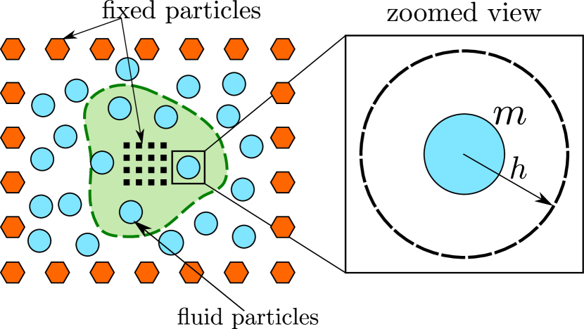
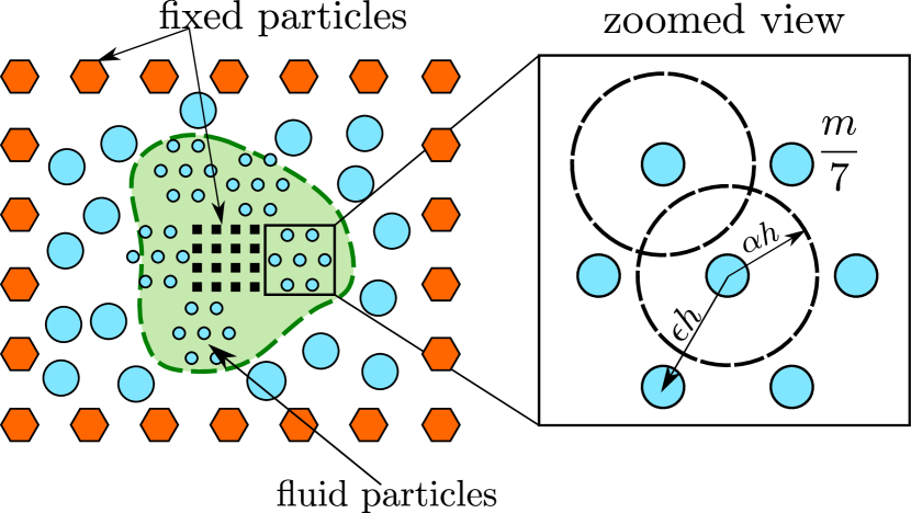
Algorithm 2 describes the splitting procedure which follows Feldman and Bonet [42] and Vacondio et al. [47]. Figure 1 shows an illustration of the splitting algorithm. The orange hexagonal particles indicate the outer boundary or the edge of the fixed internal domain, the black square particles correspond to solid particles. Both the orange hexagonal and the black square particles constitute the fixed particles and will not subdivide. The blue particles correspond to the fluid particles and are non-fixed as they may subdivide. The green zone indicates the region having maximum mass . If a particle exceeds its maximum mass, we split the particle into 7 daughter particles, where we place 6 daughter particles on the vertices of a hexagon, at a distance of times the smoothing length away from the original particle, centered around the location of the original particle. We place the daughter particle at the location of the original particle. The daughter particles’ smoothing length is set to times that of the original particle smoothing length.
The merging algorithm follows Vacondio et al. [43] although with some differences that allow us to perform this in parallel. In a single iteration, a particle may merge only with one other particle. Two particles merge if the distance between the two is less than the mean smoothing length of the two , and the sum of mass of the two particles is less than the maximum of the of either of the particles , and is closest to particle . This is fully parallel, since the particle will only merge with particle if particle is to merge with particle . We place the merged particle at,
| (32) |
where is the mass of the merged particle. Set the velocity using the mass-weighted mean as,
| (33) |
similarly update other scalar properties, like, pressure, and transport velocity. Set the smoothing radius using [43],
| (34) |
where is the kernel function and is the number of spatial dimensions. The pseudo-code for the algorithm is given in algorithm 3. Note that when merging the particles, the particle with the smaller index is the one that is retained.
After finishing the splitting, we run the merging algorithm iteratively for three times. After this, the smoothing length of all the particles is reset to the value corresponding to the average mass of the neighbors,
| (35) |
where is a constant corresponding to the value of smoothing length factor used in the simulation. In our simulations we set this value to 1.2 for the quintic spline kernel.
We employ shifting after our adaptive refinement procedure. The new position of the particle is given by,
| (36) |
we correct the fluid properties by using a Taylor series approximation. Consider a fluid property the corrected value after shifting is obtained by,
| (37) |
Algorithm 4 summarizes the adaptive particle refinement method. First, we set the of all the fluid particles in the neighborhood of a boundary to the resolution of the boundary. Next, we set of all the particles which satisfy specific criteria to the highest resolution. This is useful to define solution adaptivity, where a particular flow feature is monitored, and particles exceeding specific tolerance criteria are refined to the highest resolution. After that, we run the update spacing algorithm algorithm 1 which updates the of all the fluid particles. Then follows the splitting and merging procedure as described above.
The algorithms for the solution adaptivity are the same as that used in the original work of Muta and Ramachandran [1] with the difference that the properties are directly set on the fluid particles and not on the background particles. In the present work we use the vorticity to determine solution adaptivity.
3.1 Implementation in PySPH
PySPH is an open-source, Python-based, multi-CPU, and GPU framework for SPH simulations. We have used the Python based interfaces PySPH provides to implement most of our adaptive algorithm. PySPH exposes Python-friendly interface to the user and using internal mechanism generates a high performance serial or parallel code based on the choice of the user. For an overview of the PySPH design, see Ramachandran et al. [49] and https://pysph.readthedocs.io for a detailed reference.
We use the Tool interface to split and merge the particles. The Tool interface provides a way for a user defined callback to run before or after the integration stages by overloading the pre_stage or post_stage methods, respectively. It also provides a way to run a user callback before the start of the integration step by overloading the pre_step method. Listing LABEL:lst:tool shows a sample Python code used in our adaptive particle refinement algorithm. The class AdaptiveResolution overloads the pre_step method of Tool to run a user callback self.run which in turn calls other specific functions related to splitting, merging, and shifting.
These functionalities enable one to write the code without having to pay much attention to the low-level high-performance complexities of implementing on different platforms like multi-core CPUs, or GPUs. The respective splitting and merging algorithms are all implemented in pure Python. For complete details of our implementation one can see the source code provided in https://gitlab.com/pypr/asph_motion.
In section 5.4 we solve a case with a stationary cylinder and another with a moving square to demonstrate that we do not require the background particles. In section 5.6 we demonstrate the parallel performance of our algorithms by solving a problem and studying the speedup obtained as we increase the number of threads.
4 Source files description
The algorithms mentioned in the manuscript are primarily contained in the following files located in the code/ directory: edac.py, adapt.py, adaptv.py, and no_bg.py. The hybrid_inlet_outlet.py contains the code which implements the no-reflection boundary conditions of [62] and manages the inlet/outlet particles.
We use automan [50] Python package to automate all of our results. The file automate.py contains the code to generate all the results used in this paper. See README.md for more details regarding the individual run time of the problems in automate.py. The following files in the code/ directory contain the test problems used in the manuscript:
-
1.
fpc_auto.py: Flow past a stationary cylinder.
-
2.
moving_square.py: Flow past a moving square (SPHERIC test 6).
-
3.
ellipse_plunging.py: Flow past a plunging ellipse at Re = 500.
-
4.
ellipse_tranlation.py: Flow past a translating ellipse at Re = 500.
-
5.
fpc_bao_static.py: Flow past two stationary cylinders at Re = 100.
-
6.
fpc_bao_oscillation_1cylinder.py: Flow past single oscillating cylinder at Re = 100.
-
7.
airfoil_stationary_naca.py: Flow past a stationary NACA5515 airfoil.
-
8.
s_shape.py: Flow past a rotating S-shape at Re = 2000.
-
9.
sun_airfoil08_aoa4.py: Flow past a NACA0008 airfoil at angle of attack and Re = 2000.
-
10.
sun_airfoil12_aoa6.py: Flow past a NACA0012 airfoil at angle of attack and Re = 6000.
-
11.
performance.py: Code to measure the parallel performance of the algorithms.
5 Results and Discussion
In this section we demonstrate practical applications of the adaptive smoothed particle hydrodynamics method for selected problems in two dimensions. The problems considered are fairly challenging to solve without the adaptive refinement. We consider moving and stationary geometries specifically focusing on the following problems:
-
1.
flow around two stationary cylinders in a side-by-side configuration with different gap spacings;
-
2.
flow over airfoils with different NACA profile at different Reynolds numbers and angles of attack;
-
3.
flow around a moving square at different Reynolds numbers; and,
-
4.
flow around a single oscillating cylinder with different oscillating frequencies.
5.1 Flow around two stationary cylinders in a side-by-side configuration
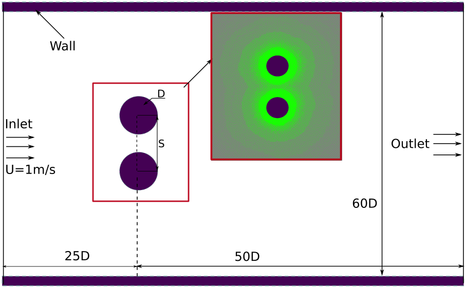
We study the flow around two stationary cylinders in a side-by-side configuration at . The flow produces distinct wake patterns at different gap spacing between the cylinders. This problem is studied first by Kang [64] and further used as a validation test case by Bao et al. [65] but do not have SPH related studies. The diameter of each of the cylinders is . The dimensions of the computational domain are based on , and the schematic diagram of the computational domain is shown in fig. 2. For each inlet, outlet, and wall, we use layers of particles to get full kernel support. Three different cases of center-to-center cylinder spacing and are considered for simulations. A constant velocity is prescribed at the inlet, , and the kinematic viscosity is given by . Other geometric and numerical parameters are provided in Table 1.
| Parameter | Value | Parameter | Value |
|---|---|---|---|
For all the cases, we deploy particles in the range of to on a m m domain. The maximum spacing of fluid particles is and the minimum resolution of the fluid particles, which also matches the resolution of the boundary, is ; the ratio of which is times smaller. Without an adaptive resolution, the problem would need million particles to simulate at such accuracy using the minimum resolution.
We are able to observe the three kinds of vortex shedding wake patterns that occur for each configuration. The wake patterns are (i) single bluff body at , (ii) a random flip-flopping gap at , and (iii) anti-phase synchronized wake at . Time evolution of the simulated results of total drag and lift force coefficients are presented in figs. 3, 4 and 5. The simulations took a fairly long wall-clock time for seconds of simulation time, each case requiring an average wall-clock time of hours on a server with cores and threads for the adopted resolution.
Figure 3 shows the comparison of time history of the coefficients of total drag and lift for spacing up to . The figure illustrates the force characteristics of a single bluff body type with entirely suppressed gap flow observed at .
Our results show a phase difference which may be caused by the differences in the nature of the solvers, time-stepping used, and boundary conditions. The results are in good agreement with the reference data of [65]. The trend, as well as the magnitude of the curves, is matching well.
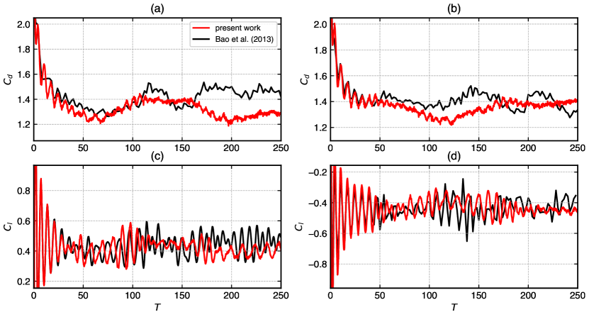
Figure 4 shows the force characteristics for the spacing . The flow is complicated and belong to a randomly flip-flopping flow for which the wake pattern looks irregular [65]. Our results compare very well at the beginning up to around seconds of the flow. The results show some discrepancy in the afterward but stay in the trend, matching the amplitude and frequency. The results match better than the in all the cases for both the top as well as bottom cylinders.
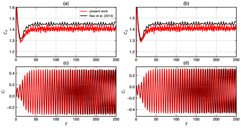
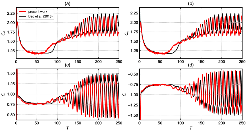
Figure 5 displays the comparison of results for the coefficients drag and lift force at spacing . The results are matching well with the of the reference data in fig. 5 (a) and fig. 5 (b) of the upper and lower cylinders with differences less than percent. The results of are in a very good agreement as shown in fig. 5 (c) and fig. 5 (d) for both the cylinders. The force characteristics of the flow at this gap between the cylinders is anti-phase synchronized where the vortex is shed behind each cylinder independently and symmetrical to the centerline.
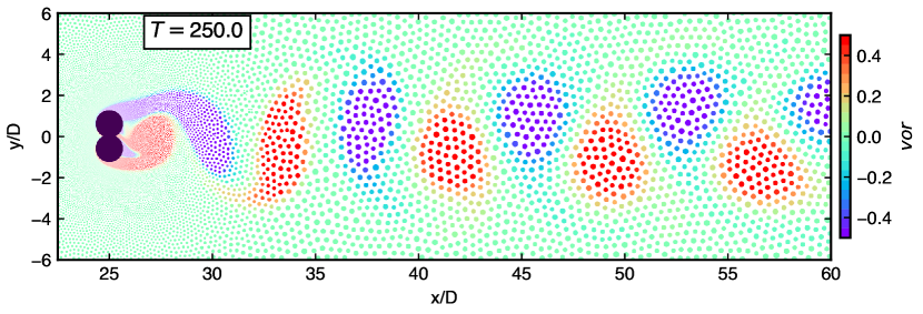
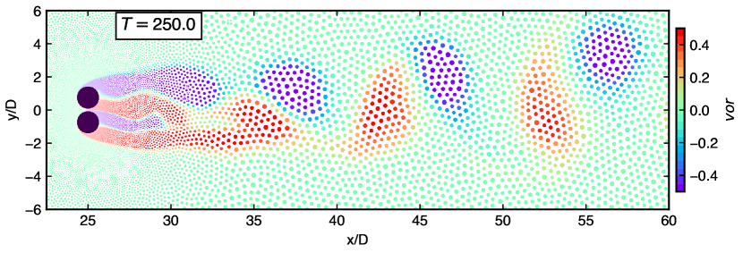
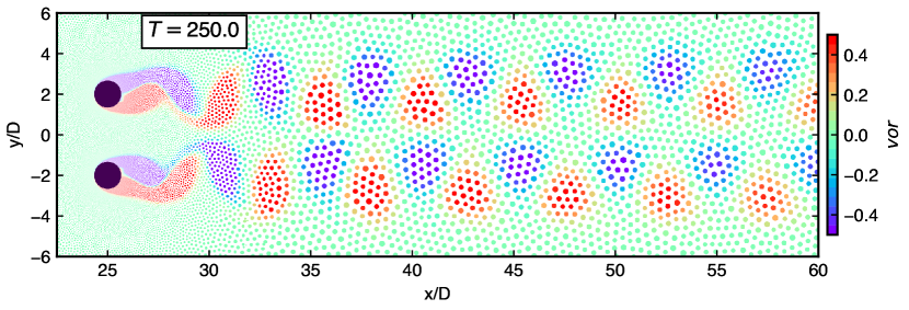
Figure 6 exhibits the vorticity distribution corresponding to the three spacing ratios. The results indicate that the flow characteristics and wake structure explained in Figs. 3 to 5 are justified. The flow structure strongly depends on the spacing gap for the given Reynolds number. A suppressed flow, seemingly a single bluff-body wake pattern is shown by the smallest spacing of in fig. 6(a). In fig. 6(b) the gap flow flip-flops for and seems irregular. The wake pattern changes to a synchronized flow as the spacing increases. As shown in fig. 6(c), the instantaneous wake is anti-phase synchronized; the vortex shedding occurs completely behind each cylinder which is symmetric with the wake centerline.
The behaviour of the flows around two stationary cylinders and a single oscillating cylinder, or both is helpful to understand the mechanism of flow around two or more oscillating cylinders. The present SPH model is able to simulate and accurately identify the wake characteristics of the flow. The force quantities are in general in good agreement with the results available in the literature. This accuracy is achieved with a proper particle resolution using a reduced total number of particles.
5.2 Flow over airfoils with NACA profile
Flow around airfoil present difficulties to conduct high accuracy SPH simulation. It can be more difficult when it is thinner, particle distribution is irregular, or if it is moving. It is further challenging in complex motion applications like in a rotational motion, elliptic motion, and motions which combine heaving, oscillation, and pitching. One of the first applications of SPH to model flow around an airfoil was conducted by Shadloo et al. [66] and [67] in which they have shown a comparative study between the weakly compressible and incompressible SPH methods. However, their results have shown poor accuracy even when employing large number of particles at moderate Reynolds number. With the help of multi-resolution and particle shifting technique, Sun et al. [68] indicated an improved success of airfoil SPH simulation for Reynolds number up to . Huang et al. [20] illustrated an improved simulation of viscous fluid flow around airfoils using SPH scheme possessing iterative particle shifting technology (IPST) and which does not use kernel gradients. The numerical study of airfoil motion is important for application like in unmanned aerial vehicles (UAVs) for thrust generation and in vertical axis wind turbines (VAWTs) for power optimization.
We discuss three stationary airfoil cases: (i) NACA5515 airfoil at and , (ii) NACA0008 at and , (iii) NACA0008 at and . The computational domain is , where m is the characteristic length (chord) with center at the airfoil midpoint. The algorithm of Negi and Ramachandran [63] is used for packing the airfoils.
5.2.1 NACA5515 airfoil at and
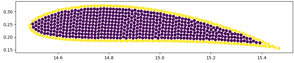
Figure 7 depicts boundary points of NACA5515 marked in yellow color and inner particles of the solid in violet. The particles on surface of the airfoil (boundary points) are identified by computing divergence of the position vector. All the surface points are identified correctly when the computed value is lower than , is the dimension. The airfoil particles are packed with the smallest spacing, , which is equal to the minimum resolution of fluid particles for mapping. We have simulated for and compared the results with [20].
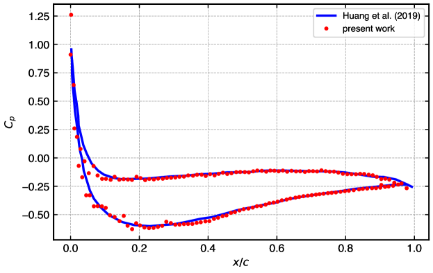
Figure 8 shows the coefficient of pressure on the surface of an airfoil with the NACA5515 profile. The airfoil is at an angle of attack , and uses particle spacing . The simulated result of the present model agrees very well with [20]. Based on the information provided in [20], about particles are employed to produce their result. However, our solution require around particles which could be considered as a massive gain due to the adaptive resolution.
5.2.2 NACA0008 airfoil at , and
The airfoil in NACA0008 profile has very thin cross-section which makes it a challenging problem for numerical methods. This section discusses the flow around the airfoil at an angle of attack . We simulate the problem for two different Reynolds numbers which are and . The total drag and lift coefficient of the simulated results are compared with Diffused Vortex Hydrodynamics (DVH) method of Rossi et al. [69], and SPH method of Sun et al. [68].
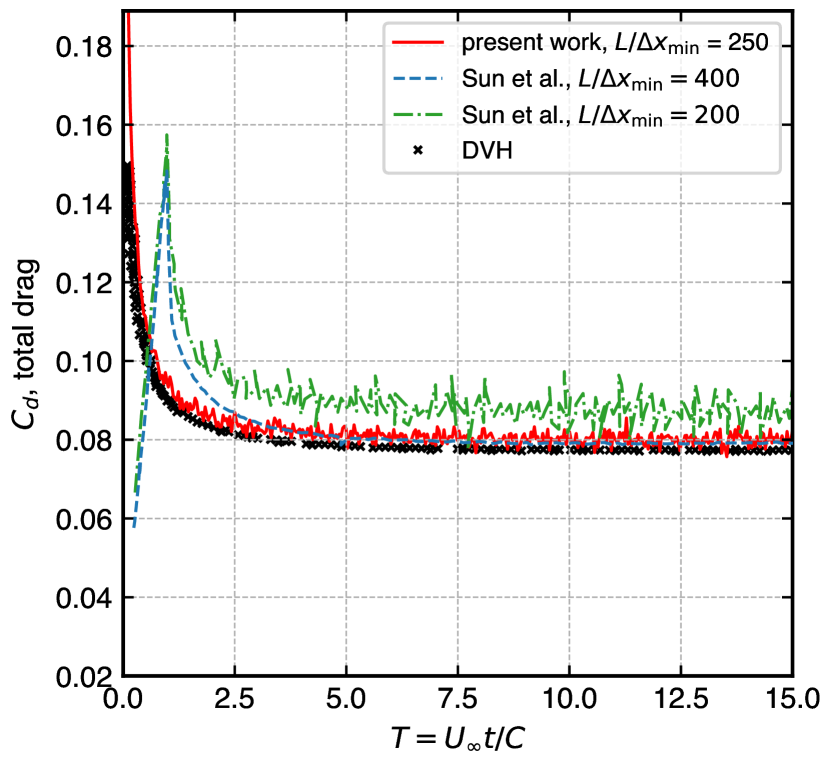
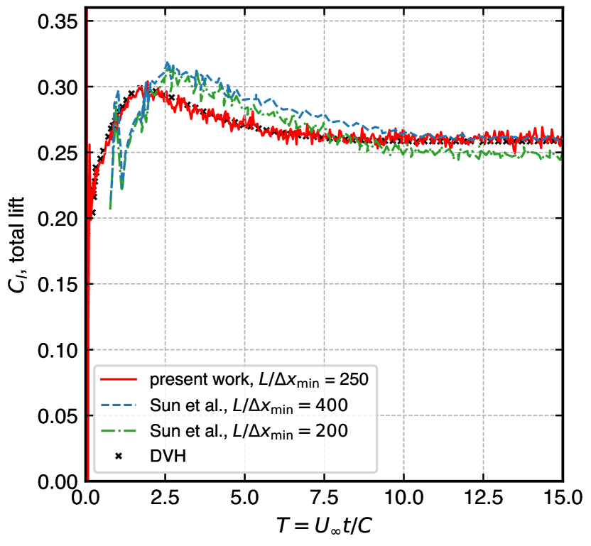
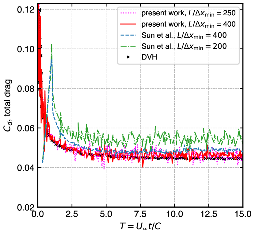
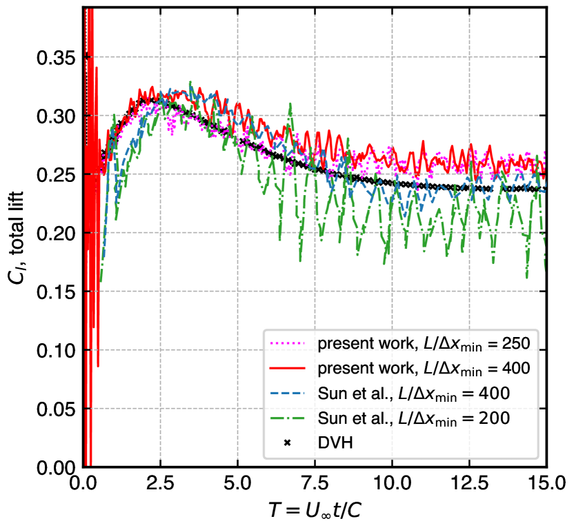
Figure 9 illustrates the evolution of force coefficients drag (left) and lift (right). We simulate for using for (top) and for (bottom). At this resolution our simulations show very good comparison with DVH [69] and have improved results compared with [68]. The trend of the curve is captured very well except some oscillations that can be minimized by increasing the resolution. Sun et al.’s result of comparable resolution has higher noise and misses some features of the curve. Also, the number of particles (from Sun et al.’s Fig. 3) is more than particles for , whereas our adaptive EDAC-SPH simulation employs around particles.
Table 2 shows the number of particles used in the simulation for two different Reynolds numbers. The number of particles is about times less than [68].
| Method | |||
|---|---|---|---|
| Sun et al. [68] | |||
| Adaptive EDAC-SPH | |||
| Adaptive EDAC-SPH (solution adaptivity) | — |
We ran the case with and without solution adaptivity, where the vorticity particles exceeding 5% of the maximum vorticity in the domain are refined to the highest resolution. The number of particles increases to 260k. There is no significant difference in the lift or drag coefficient of the airfoil between the solution adaptive and without the solution adaptive case since the solid bodies are initially discretized at the highest resolution. Our non-solution adaptivity case took about 18 hrs, whereas the solution adaptivity case took about 41 hrs.
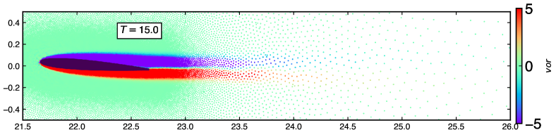
In fig. 10, we display the vorticity field around NACA0008 airfoil at an angle of attack . The top figure is simulated without solution adaptivity at , and the bottom is simulated using solution adaptivity at . Due to the small angle of attack, the viscous flow remains attached to the surface where a steady regime has reached immediately. The selected airfoil configuration has practical application in micro-aerial vehicles (MAVs) for the Reynolds numbers in the given range [69].
5.3 Flow around a moving square
The flow around a moving square represents a simple geometry but a flow situation that can be very complex due to the sharp edges. The problem consists of a square geometry moving through a stationary fluid kept inside a rectangular box. The test can generate intense unsteady vorticity and has been a challenging test case for SPH solvers. This simulation is part of a validation test suite compiled by the SPH rEsearch and engineeRing International Community (SPHERIC) [70]. The benchmark results of this test case are simulated using Finite Difference Navier-Stoked (FDNS) solver by [71]. In SPH [43], and [72] studied this problem. We study the time histories for the drag force coefficients (pressure, viscous or total) and the generation and diffusion of vorticity.
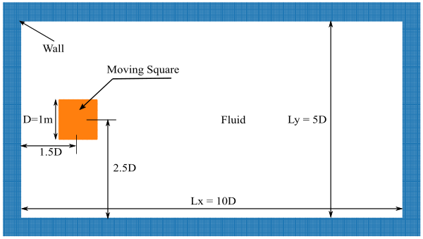
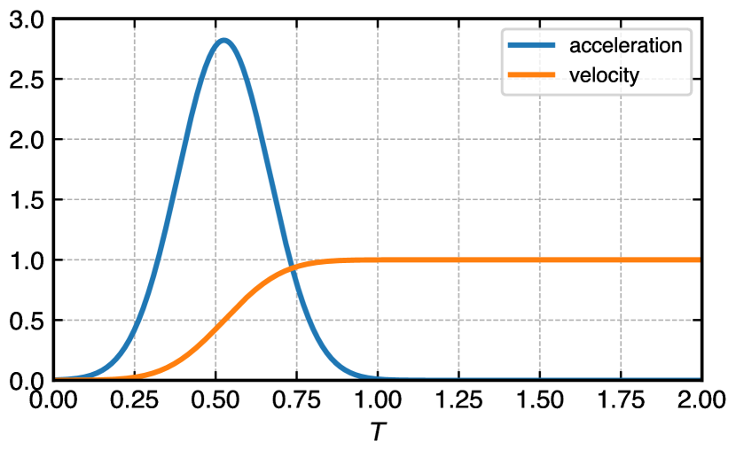
The geometric configuration is shown in fig. 11(a) at time . The body motion in time is shown in fig. 11(b). The domain size is m m, with the square obstacle having a length of 1m. The square motion is prescribed with a smooth acceleration in the -axis starting from rest until it reaches a steady maximum velocity . The boundary conditions are no-slip and no-reflection on all walls of the rectangular domain and slip velocity on the solid square. The simulation is conducted for a Reynolds number of with no gravity force and zero initial pressure field for the viscous incompressible Newtonian fluid of density .
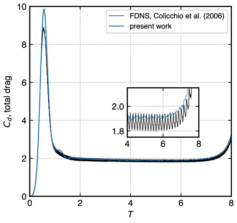
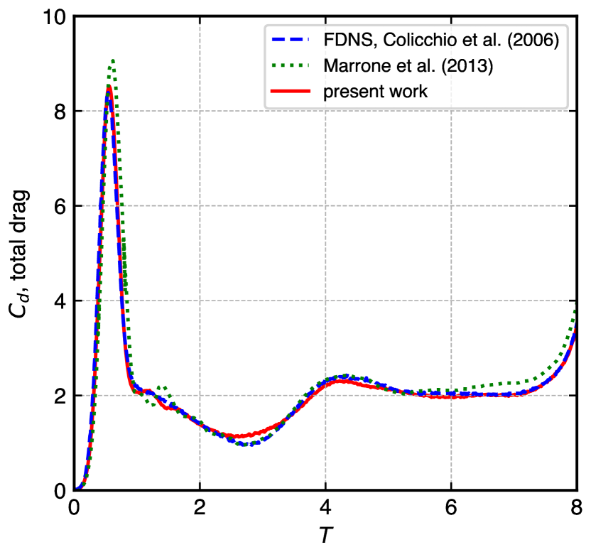
In fig. 12, we show the time evolution of the drag coefficient of a moving square at (a) using and (b) at a slightly higher of using . Simulated results obtained from the present method are compared with the results of the FDNS solver [71] and Marrone et al. [72]. The comparison shows, especially with FDNS, very good agreement with all the necessary features.
The simulation requires fluid particles using adaptive resolution for the converged solution. The initial spacing of particles on the domain is ; the smallest spacing is near the obstacle. The solid particles are packed using the minimum resolution to create a mapping in the fluid-solid interface. If the was used in the entire domain, would be which produces as the total number of particles. However, with an adaptive particle resolution, we have used only particles to produce accurate results. This substantially reduces the number of particles by times when compared with Marrone et al., [72] and by four times when compared with the results by [71].
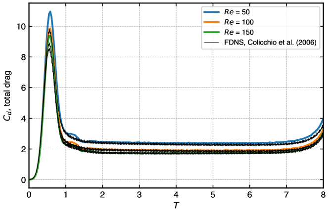
Figure 13 shows the variation of drag coefficient for flow around a moving square at different Reynolds numbers. The comparison is made for three Reynolds numbers of , , and . The results of the adaptive EDAC-SPH are in good agreement with [71] results. However, due to numerical reasons [71] show the small amplitude and high-frequency oscillations which are avoided in our case.
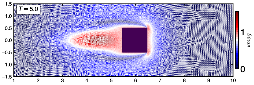
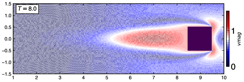
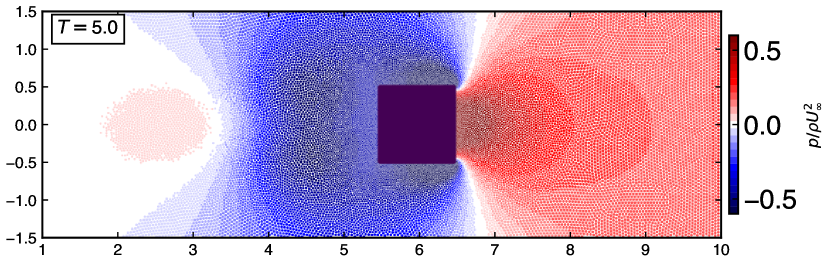
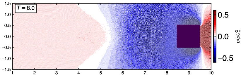
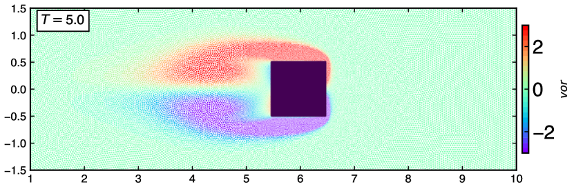
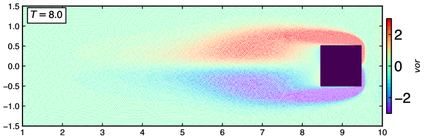
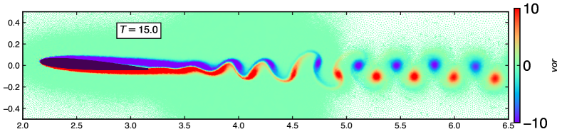
Figure 14 show the particle distribution with color indicating pressure, vorticity and velocity magnitude taken at and . The qualitative observations illustrate the generation, diffusion, and convection of the unsteady vorticity proving the capability of the adaptive EDAC-SPH scheme.
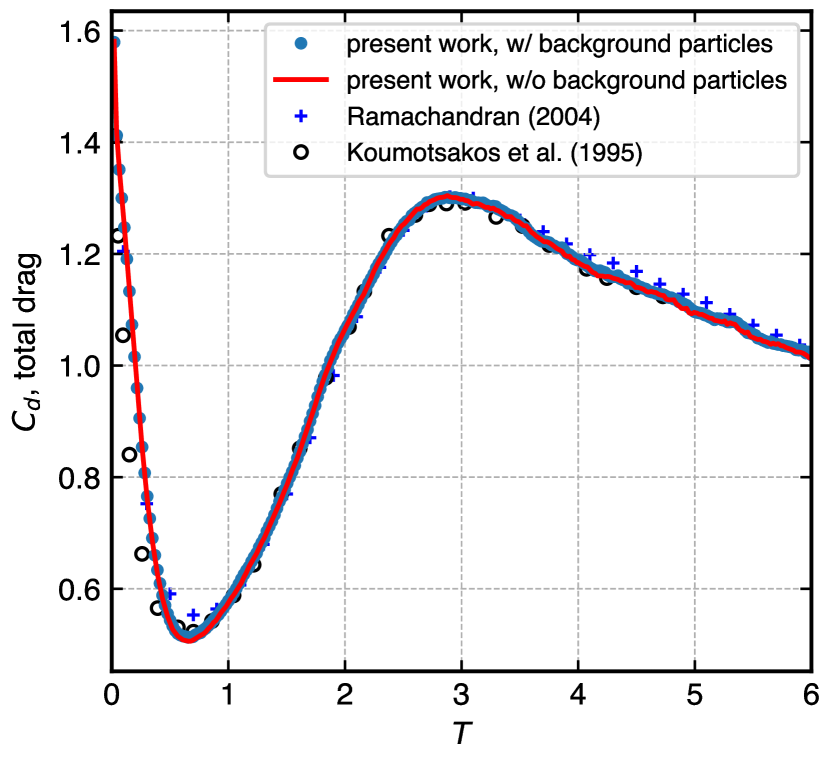
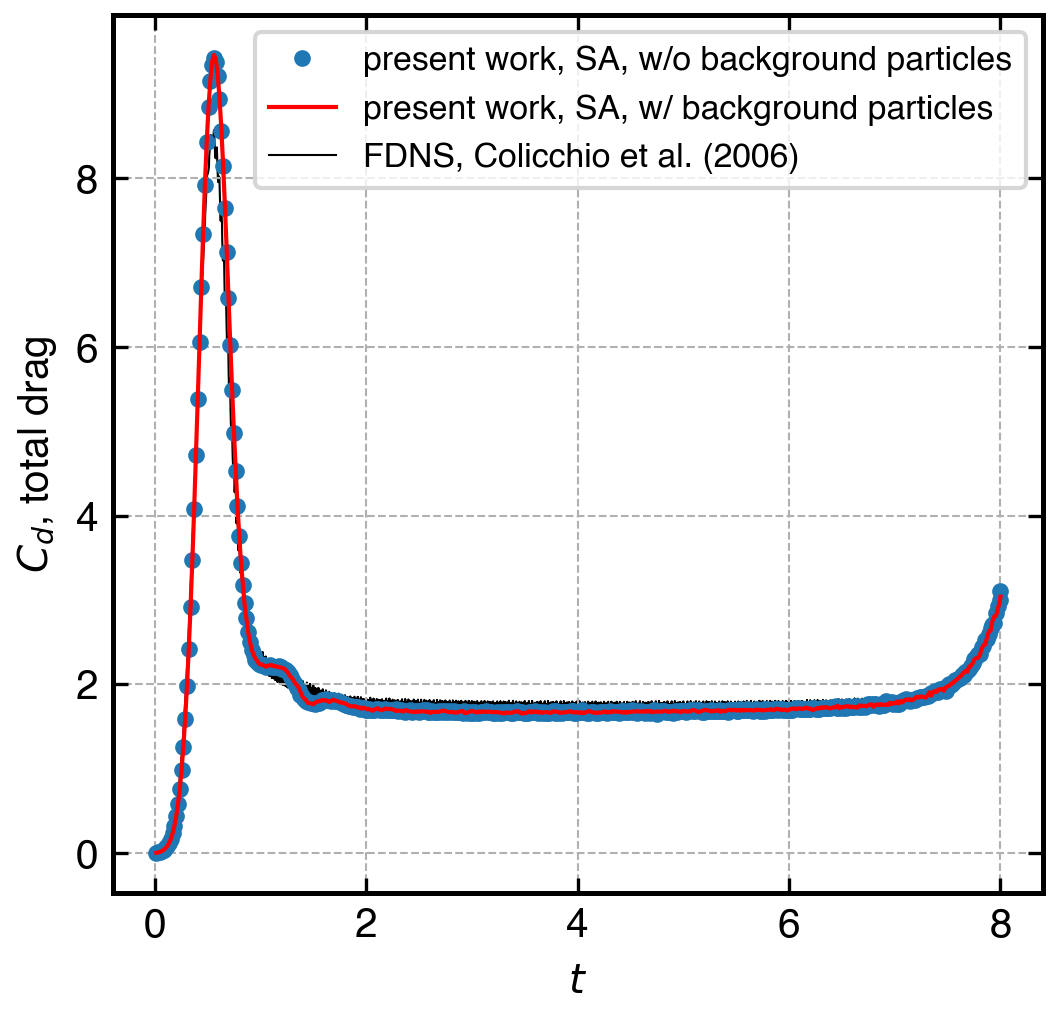
5.4 Removal of background particles
Muta and Ramachandran [1] used a collection of particles called “background” particles to define the particle spacing and reference mass. But in this work, we show that the background particles are not necessary to set this reference mass. Updating the reference mass on the particles themselves produces results closely matching those produced by the original algorithm using background particles. This reduces memory usage by removing background particles’s storage, and a small reduction in the computational time. We perform two simulations to establish the no background particle approach. We first consider the flow past a circular cylinder at , the simulation parameters and domain sizes are the same as defined in [1]. Furthermore, we compare the results with the established vortex method results [73, 74]. We then consider the flow past a moving square in a box at . Refer to section 5.3 for the simulation parameters. We compare the results to the incompressible FDNS simulation results [71]. In this case, the geometry is moving. In addition, we use solution adaptivity to refine the particles to the lowest resolution where the vorticity exceeds 5% of the maximum vorticity in the simulation.
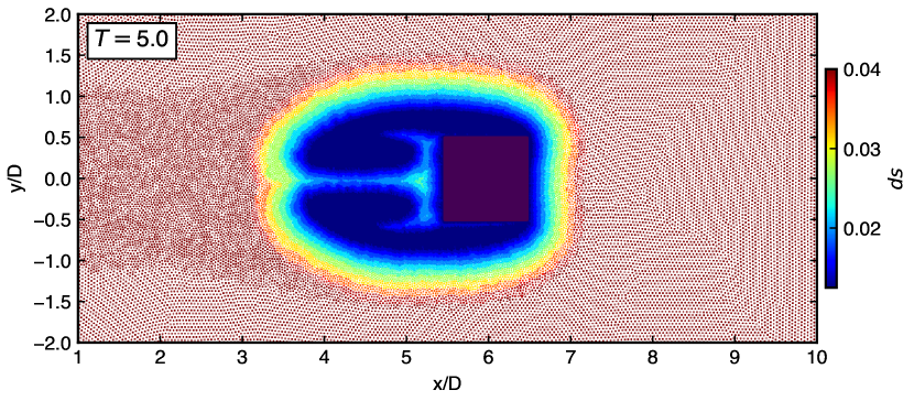
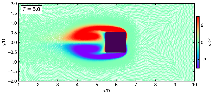
Figure 15(a) shows the time history of the drag coefficient of the flow past cylinder problem without solution adaptivity. The results of adaptive EDAC-SPH are computed with and without use of background particles, and both results match very well with the reference data from vortex method simulations. Figure 15(b) shows the time history of the drag coefficient of the moving square problem using solution adaptivity. This further confirms a good match when not using the background particles. Figure 16(a) we show the distribution of the spacing without using background particles and in fig. 16(b) we show the vorticity distribution. It can be seen that the regions satisfying the solution adaptivity criteria are refined to the highest resolution, and the particles closest to the solid square particles are refined to the highest level.
5.5 Flow around an oscillating single cylinder
The numerical examination of flow around an oscillating single cylinder is helpful for the simulation and deeper analysis of two or more oscillating cylinders. The study of flow over a cylinder is important for the study and design of flow over a car, flow over aircraft, flow over airfoil blades, or flow over a pillar for the design of bridges [64, 65, 75, 76, 77].
Bao et al., [65] classify the flow around the oscillatory motion of cylinders into lock-on and unlock-on states which are also characteristic of two cylinder flows. The classification depends on the shedding and oscillating frequencies for which the transition occurs around a frequency ratio of one.
We analyze the oscillatory motion of a single cylinder subject to cross-flow at . The sinusoidal motion of the cylinder is defined by , where is the amplitude, the angular velocity, and the frequency of oscillation. Two amplitudes of oscillation (low and high) and frequency ratio ranging from low to high are chosen for the simulation. Here , where is a natural vortex shedding which is for a single cylinder oscillating at . The values are and .
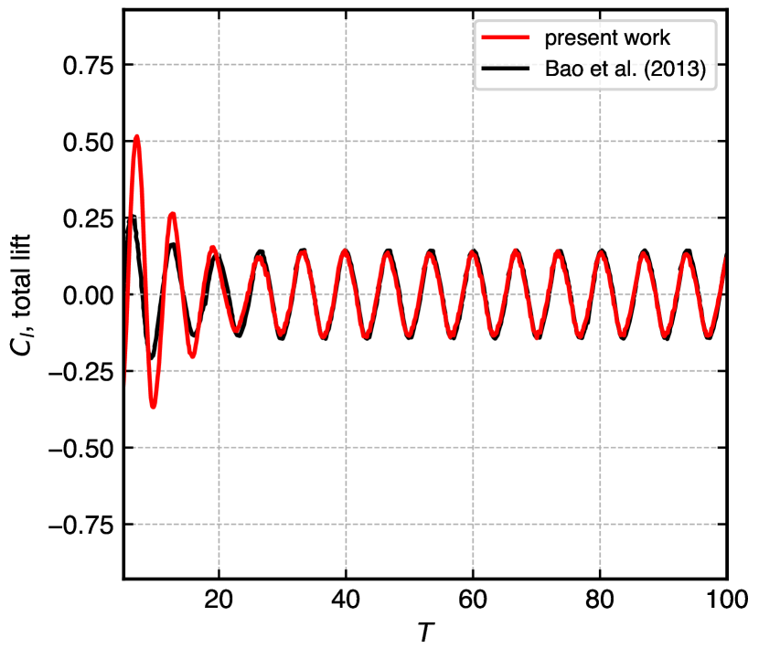
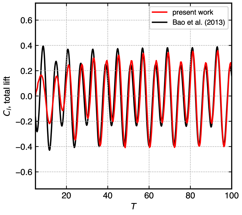
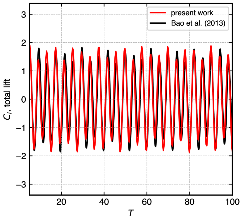
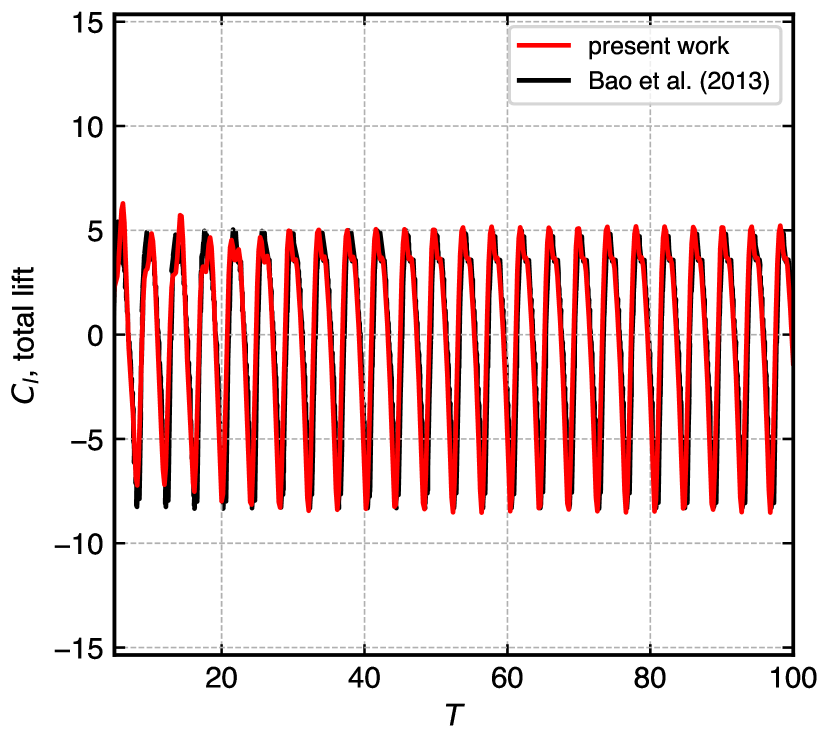
Figure 17 shows the time history of the fluctuating lift coefficient for four combinations of amplitude and oscillation frequency. The range includes lock-on and unlock-on states. In fig. 17(a) , the simulated results initially show faster transition and match with [65] capturing the peak-to-peak amplitude and all trends. In fig. 17(b) , our simulation depicts pure sinusoidal oscillation from the beginning, matching very well for seconds. The fluctuating lift coefficient beats with a stronger magnitude for higher oscillating frequencies. Figure 17(c) , takes a combination of the smallest amplitude ratio with the highest value of the oscillating frequency, the results match very well from the beginning. In fig. 17(d) , both parameters of the amplitude and oscillating frequency are on the higher side. The results of this simulation capture all the trends and peaks of the lift coefficients fluctuation and are in good comparison with the reference data.
5.6 Performance analysis
In this section, we discuss the parallel performance of the adaptive EDAC-SPH implemented using the framework of PySPH. To show that our adaptive algorithm is fully parallel, we run the moving square test case with the highest resolution of and the lowest resolution of , giving us 57k particles. As opposed to the gradual start in the moving square problem described in section 5.3 we move the solid with a uniform velocity of 1 ms-1. We proceed to test this problem on a 6-Core Intel Core i7 CPU. We compare the time taken to run 1000 time-steps on a serial single-core single-thread execution with a parallel (OpenMP) execution on the multi-core CPU with 4-threads and 6-threads.
| Component | 1-thread | 4-threads | 6-threads |
|---|---|---|---|
| splitting & merging | 24.74 s | 7.91 s | 6.64 s |
| removing & adding particles | 0.63 s | 0.61 s | 0.70 s |
| EDAC scheme | 260.77 s | 78.44 s | 64.38 s |
Table 3 shows the time taken by various algorithms described in this manuscript along with the time taken by the adaptive EDAC-SPH scheme. The splitting and merging component constitutes the Update Spacing algorithm 1, splitting algorithm 2, and merging algorithm 3; the removing and adding of particles constitutes for the time taken by the removal of the merged particles’ indices from the data structure, and addition of new particles to the data structure; the EDAC scheme constitutes the overall time taken by the SPH formulation.
Table 3 shows that the multi-thread implementation scales well in parallel with a scale-up of 3.13x on 4-threads and 3.73x on 6-threads. The time taken for removing and adding particles to the data structure constitutes less than 2.5% of the adaptive algorithm and this process is serial in execution. The present scheme again scales well with an increase in number of threads. The scale-up is 3.32x on 4-threads and 4.05x on 6-threads. The parallel execution of the adaptive algorithm constitutes 10–11% of the adaptive EDAC-SPH scheme.
The results of this section validate our formulation with the existing numerical simulations.
6 Complex motion demonstration
Simulation of fluid flow around moving solid bodies is challenging and even more challenging in complex motion scenarios such as the rotation of a complex geometry and motions that combine pitching and translating. The adopted adaptive EDAC-SPH method automatically refines the particles around solid bodies performing any type of motion. Applications in complex moving cases are demonstrated in this section. We consider the following examples for the demonstration:
-
1.
translating and pitching ellipse;
-
2.
plunging ellipse with elliptical motion trajectory; and,
-
3.
rotating S shape.
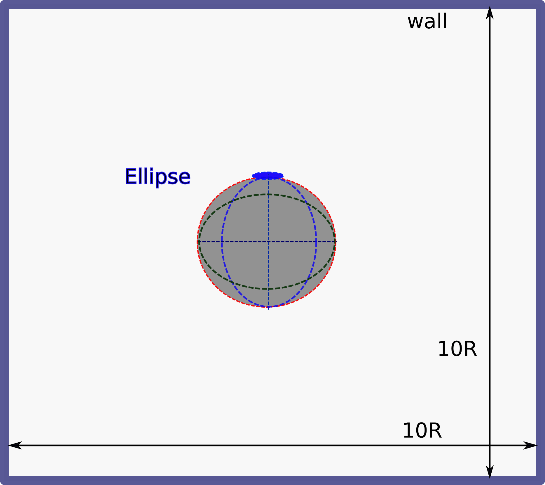
An elliptic solid body and an S shape are used to illustrate the various motions. The ellipse has a characteristic length of m and axis ratio . All the test cases use boundary conditions of the moving square problem discussed in section 5.3 for a stationary fluid.
6.1 Translating and pitching ellipse
The acceleration of the center of mass of the ellipse, , and the instantaneous pitch angle with respect to the horizontal, , are given by,
| (38) |
| (39) |
where , , , , and the pitch amplitude are the constants.
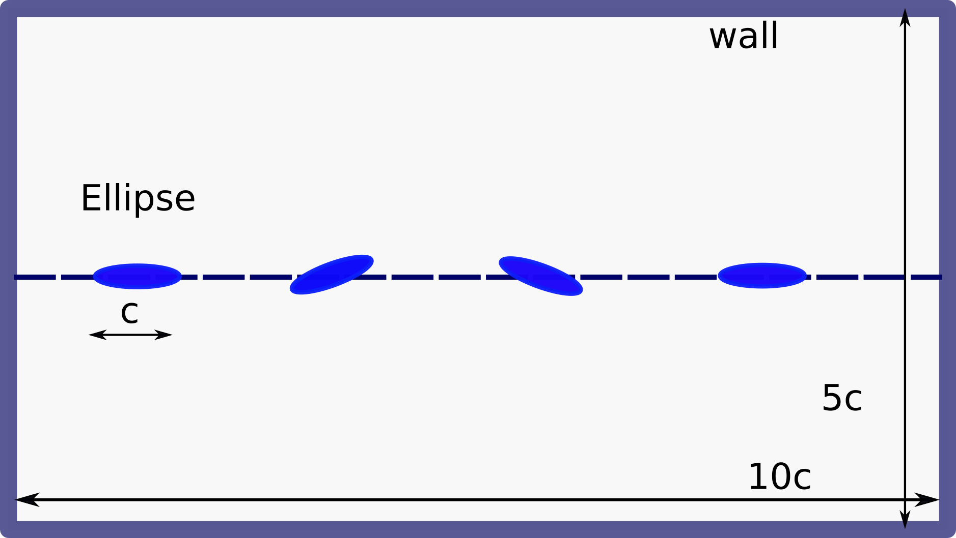
We simulate the translating and pitching ellipse in a rectangular domain of size at a Reynolds number of . The ellipse is started with a smooth acceleration in the -axis starting from rest until it reaches a steady maximum velocity of 1 m s-1. The schematic of the domain is shown in fig. 18. The wall boundary condition is the same as that used in the moving square problem of section 5.3.
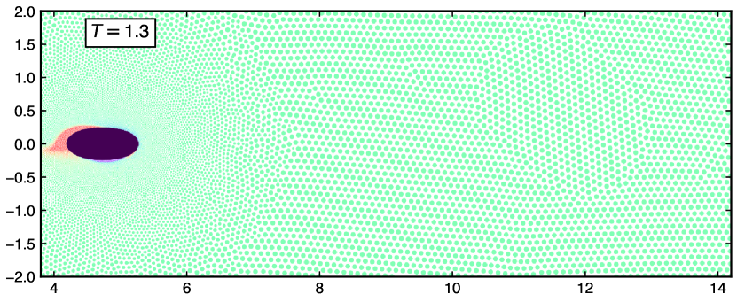
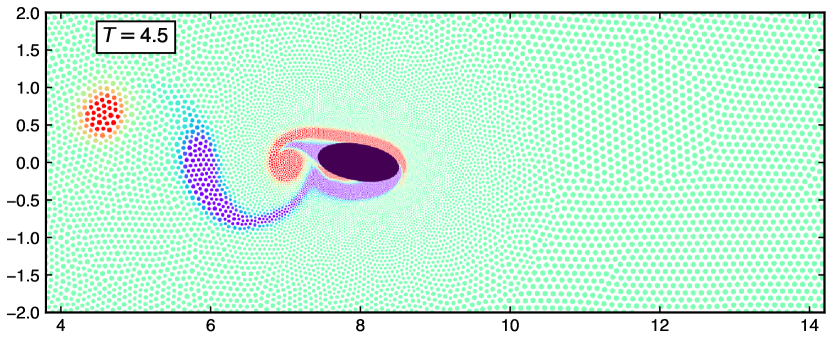
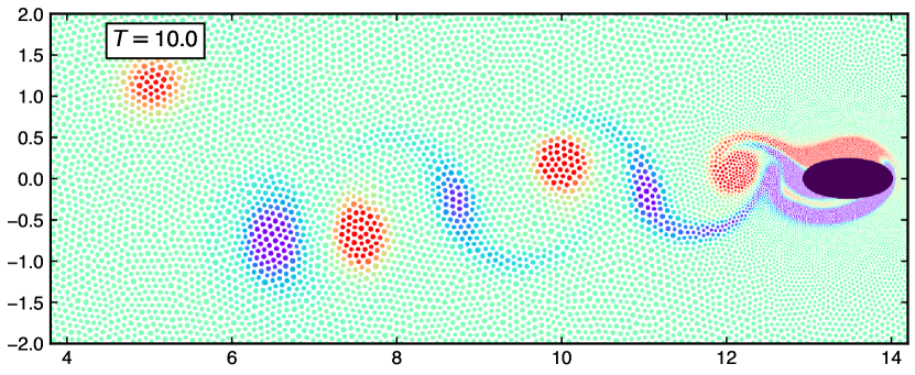
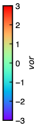
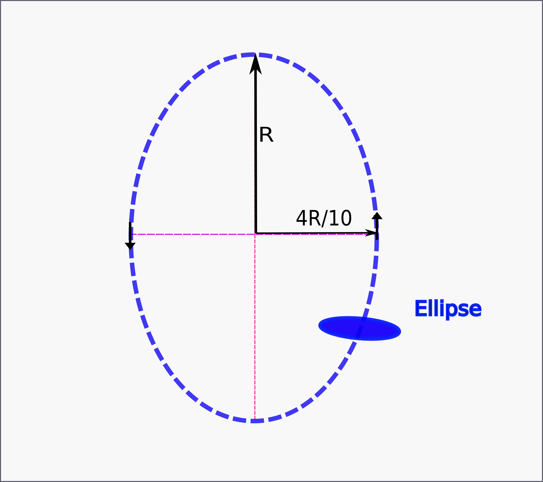
Figure 20 shows the vorticity distribution around the ellipse at different times. The top figure is at , where the ellipse is from the horizontal. The middle figure is at , where is ellipse is at from the horizontal and the bottom figure is at the final time of .
6.2 Plunging ellipse with elliptical motion trajectory
Kinematics of a flapping motion describes a vertical translation (heaving), a horizontal oscillation, and pitching rotation. The amalgamation of these motions constructs an elliptical trajectory (path) of the pitching ellipse. This kind of kinematics is seen in the flying birds, aquatic animals, and has potential applications in high-efficiency Micro Air Vehicles (MAVs), and other energy harvesting vertical axis wind turbine (VAWT) designs [78, 79, 80, 81]. The pitching orientation and angle of attack can also vary according to the type of motion undertaken for high-level performance. The schematic diagram of ellipse motion is shown in 21.
The motion equations for the vertical plunge, , and the horizontal sinusoidal motion, , of the ellipse are defined by,
| (40) |
where , is the angular velocity, and is a factor relating a horizontal motion with the vertical counterpart.
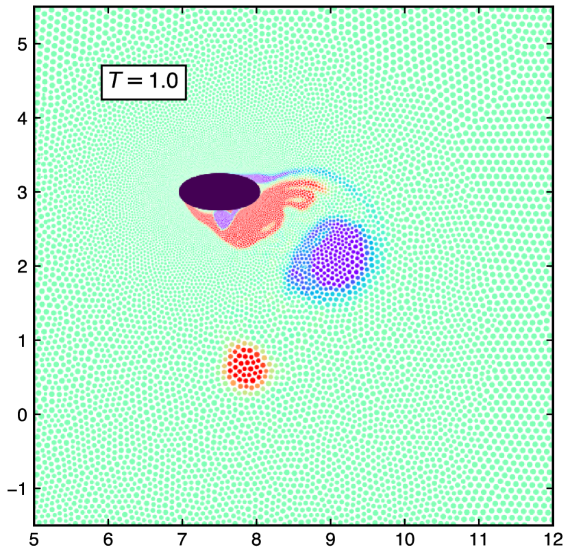
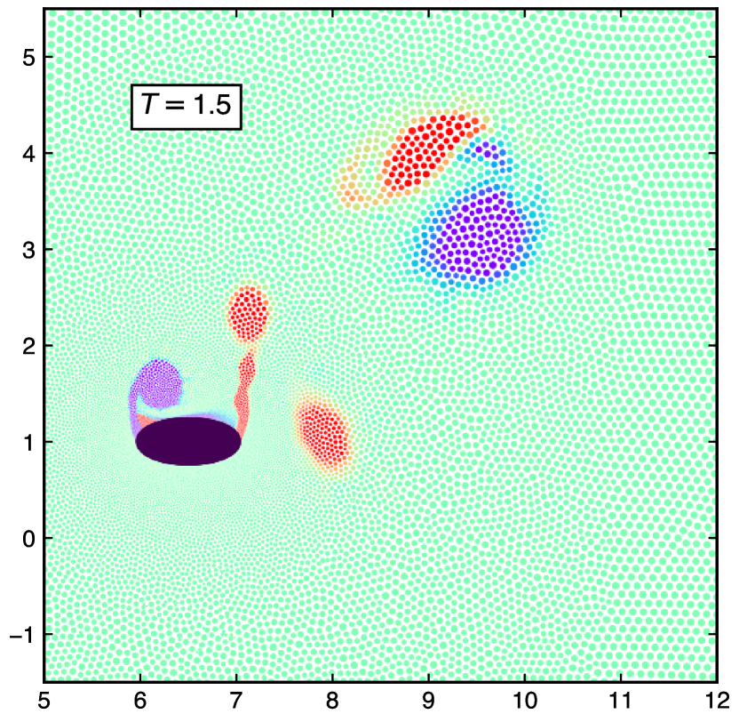
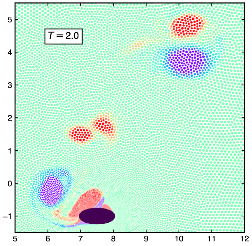
Figure 23 shows the vorticity plots of a plunging ellipse undergoing the mixed vertical-horizontal oscillatory motions forming an elliptical trajectory. The motion of the solid ellipse is described using the equations in 40, of a stationary fluid with boundary conditions discussed in 5.3. The schematic diagram of the problem is illustrates in fig 21 (a). In fig. 23(a) the ellipse is at the start of upward stroke with backward motion. In fig. 23(b) ellipse starts an upward stroke with a forward motion at period . At period , the ellipse starts the downward stroke with a forward motion. Similarly, figs. 23(c) and 23(d) show the motion of the ellipse at different time periods of , and respectively.
6.3 Rotating S-shape
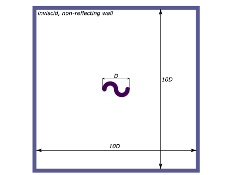
We consider a counter-clockwise rotating S-shaped body at . The outer diameter is 2 m and fig. 24 shows the domain schematic. The minimum-resolution is 10 and the maximum-resolution is 200. The body is rotated at a frequency of sec-1. We simulate the problem for sec. Figure 26 shows the vorticity distribution of the particles for the rotating S-shape at secs.
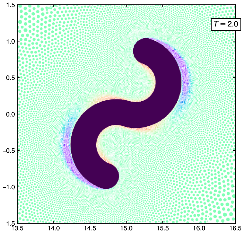
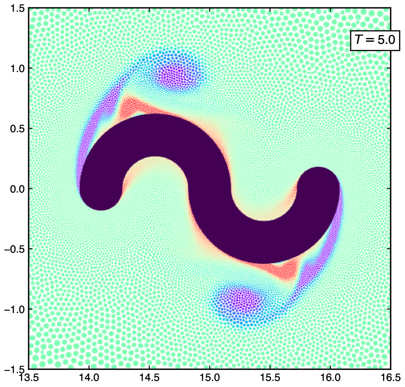
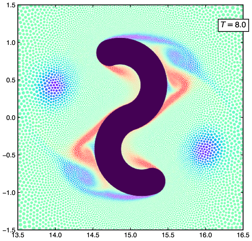
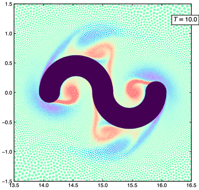
This section demonstrates the capabilities of the adaptive particle refinement in simulating complex motion and multiple bodies. This motivates further the use of adaptive EDAC-SPH in a range of applications.
7 Conclusions
In this work a modified version of the adaptive EDAC-SPH technique of Muta and Ramachandran [1] has been discussed and various applications have been demonstrated. The adaptive particle refinement is automatic; the method is efficient in terms of the number of particles that it creates and requires an optimal number of neighbors. Besides the geometry-based automatic refinement, it is possible to create static regions of refinement or use solution-based adaptivity. Unlike the original method of [1], the proposed method does not require any background particles making it more memory efficient and easier to implement. The test cases presented in this paper clearly show the applicability and computational efficiency of the method. In particular the original method did not benchmark the method for moving bodies or for multiple bodies which we do in the current work. The results show good reliability of using adaptive particle refinement in practical applications using SPH. The proposed adaptive algorithm is executed before any SPH computations are performed at every timestep. This makes it easy to incorporate into an existing non-adaptive EDAC-SPH solver.
We show how the method can be used to simulate a variety of CFD problems that involve stationary and moving geometries of varying complexity. The source code is open-source and can be obtained from https://gitlab.com/pypr/asph_motion. It is entirely written in Python and can be made to run on different platforms, like, CPU (single and multi-core), multi-CPU, as well as a GPGPU. This makes it easy for researchers to use and extend. To our knowledge this is the only open-source code available for adaptive SPH. In the future, we propose to apply this method to other practical problems. The algorithms discussed work have not been tested for three dimensional problems and this will be investigated in the future.
Acknowledgements
We would like to thank the Aerospace Computational Engine (ACE) at the Department of Aerospace Engineering, Indian Institute of Technology Bombay for providing computational resources. We would like to thank Aditya Bhosale and Miloni Atal for the parallel Octree nearest neighbor particle search algorithm in PySPH, which was essential in the scale-up study done in this paper.
References
- Muta and Ramachandran [2022] A. Muta, P. Ramachandran, Computer Methods in Applied Mechanics and Engineering 395 (2022) 115019. doi:https://doi.org/10.1016/j.cma.2022.115019.
- Bui and Nguyen [2021] H. H. Bui, G. D. Nguyen, Computers and Geotechnics 138 (2021) 104315. doi:10.1016/j.compgeo.2021.104315.
- Ye et al. [2019] T. Ye, D. Pan, C. Huang, M. Liu, Physics of Fluids 31 (2019) 011301. doi:10.1063/1.5068697.
- Lind et al. [2020] S. J. Lind, B. D. Rogers, P. K. Stansby, Proceedings of the Royal Society A: Mathematical, Physical and Engineering Sciences 476 (2020) 20190801. doi:10.1098/rspa.2019.0801.
- Vacondio et al. [2020] R. Vacondio, C. Altomare, M. De Leffe, X. Hu, D. Le Touzé, S. Lind, J.-C. Marongiu, S. Marrone, B. D. Rogers, A. Souto-Iglesias, Computational Particle Mechanics (2020). doi:10.1007/s40571-020-00354-1.
- Violeau and Rogers [2016] D. Violeau, B. D. Rogers, Journal of Hydraulic Research 54 (2016) 1–26. doi:10.1080/00221686.2015.1119209.
- Shadloo et al. [2016] M. Shadloo, G. Oger, D. Le Touzé, Computers & Fluids 136 (2016) 11–34. doi:10.1016/j.compfluid.2016.05.029.
- Lucy [1977] L. B. Lucy, The Astronomical Journal 82 (1977) 1013–1024. doi:10.1086/112164.
- Gingold and Monaghan [1977] R. A. Gingold, J. J. Monaghan, Monthly Notices of the Royal Astronomical Society 181 (1977) 375–389. doi:10.1093/mnras/181.3.375.
- Liu and Liu [2003] G. R. Liu, M. B. Liu, Smoothed Particle Hydrodynamics, World Scientific, 2003. doi:10.1142/5340.
- Monaghan [2005] J. J. Monaghan, Reports on Progress in Physics 68 (2005) 1703–1759. doi:10.1088/0034-4885/68/8/R01.
- Liu and Liu [2010] M. Liu, G. R. Liu, Archives of Computational Methods in Engineering 17 (2010) 25–76. doi:10.1007/s11831-010-9040-7.
- Violeau [2012] D. Violeau, Fluid Mechanics and the SPH Method: Theory and Applications, 1st ed ed., Oxford University Press, Oxford ; New York, 2012. doi:10.1093/acprof:oso/9780199655526.001.0001.
- Monaghan [2012] J. J. Monaghan, Annual Review of Fluid Mechanics 44 (2012) 323–346. doi:10.1146/annurev-fluid-120710-101220.
- Libersky et al. [1993] L. D. Libersky, A. G. Petschek, T. C. Carney, J. R. Hipp, F. A. Allahdadi, Journal of Computational Physics 109 (1993) 67–75. doi:10.1006/jcph.1993.1199.
- Belytschko et al. [1996] T. Belytschko, Y. Krongauz, D. Organ, M. Fleming, P. Krysl, Computer Methods in Applied Mechanics and Engineering 139 (1996) 3–47. doi:10.1016/s0045-7825(96)01078-x.
- Manenti and Ruol [2008] S. Manenti, P. Ruol, in: Proc. Int. Workshop Handling Exception in Structural Engineering, pp. 13–14.
- Khayyer et al. [2009] A. Khayyer, H. Gotoh, S. Shao, Applied Ocean Research 31 (2009) 111–131. doi:10.1016/j.apor.2009.06.003.
- Violeau and Issa [2006] D. Violeau, R. Issa, International Journal for Numerical Methods in Fluids 53 (2006) 277–304. doi:10.1002/fld.1292.
- Huang et al. [2019] C. Huang, T. Long, S. Li, M. Liu, Engineering Analysis with Boundary Elements 106 (2019) 571–587. doi:10.1016/j.enganabound.2019.06.010.
- Yang and Kong [2019] X. Yang, S.-C. Kong, Computer Physics Communications 239 (2019) 112–125. doi:10.1016/j.cpc.2019.01.002.
- Wang et al. [2016] Z.-B. Wang, R. Chen, H. Wang, Q. Liao, X. Zhu, S.-Z. Li, Applied Mathematical Modelling 40 (2016) 9625–9655. doi:10.1016/j.apm.2016.06.030.
- Monaghan [1994] J. J. Monaghan, Journal of computational physics 110 (1994) 399–406. doi:10.1006/jcph.1994.1034.
- Gotoh and Khayyer [2018] H. Gotoh, A. Khayyer, Coastal Engineering Journal 60 (2018) 79–103. doi:10.1080/21664250.2018.1436243.
- Koukouvinis et al. [2009] P. K. Koukouvinis, J. S. Anagnostopoulos, D. E. Papantonis, T. E. Simos, G. Psihoyios, C. Tsitouras, in: AIP Conference Proceedings, AIP, 2009. doi:10.1063/1.3241439.
- Monaghan [2011] J. Monaghan, European Journal of Mechanics - B/Fluids 30 (2011) 360–370. doi:10.1016/j.euromechflu.2011.04.002.
- Braun et al. [2019] S. Braun, L. Wieth, S. Holz, T. F. Dauch, M. C. Keller, G. Chaussonnet, S. Gepperth, R. Koch, H.-J. Bauer, International Journal of Multiphase Flow 114 (2019) 303–315. doi:10.1016/j.ijmultiphaseflow.2019.03.008.
- Chaussonnet et al. [2020] G. Chaussonnet, T. Dauch, M. Keller, M. Okraschevski, C. Ates, C. Schwitzke, R. Koch, H.-J. Bauer, Flow, Turbulence and Combustion 105 (2020) 1119–1147. doi:10.1007/s10494-020-00174-6.
- Wieth et al. [2016] L. Wieth, K. Kelemen, S. Braun, R. Koch, H.-J. Bauer, H. P. Schuchmann, Microfluidics and Nanofluidics 20 (2016). doi:10.1007/s10404-016-1705-6.
- Martel et al. [1994] H. Martel, P. R. Shapiro, J. V. Villumsen, H. Kang, Memorie della Societa Astronomica Italiana 65 (1994) 1061.
- Kitsionas and Whitworth [2002] S. Kitsionas, A. Whitworth, Monthly Notices of the Royal Astronomical Society 330 (2002) 129–136. doi:10.1046/j.1365-8711.2002.05115.x.
- Lastiwka et al. [2005] M. Lastiwka, N. Quinlan, M. Basa, International Journal for Numerical Methods in Fluids 47 (2005) 1403–1409. doi:10.1002/fld.891.
- Reyes Lopez and Roose [2011] Y. Reyes Lopez, D. Roose, Particle-based method II. Fundamentals and Applications (2011) 942–953.
- López et al. [2013] Y. R. López, D. Roose, C. R. Morfa, Computational Mechanics 51 (2013) 731–741. doi:10.1007/s00466-012-0748-0.
- Spreng et al. [2014] F. Spreng, D. Schnabel, A. Mueller, P. Eberhard, Computational Particle Mechanics 1 (2014) 131–145. doi:10.1007/s40571-014-0015-6.
- Barcarolo et al. [2014] D. A. Barcarolo, D. Le Touzé, G. Oger, F. De Vuyst, Journal of Computational Physics 273 (2014) 640–657. doi:10.1016/j.jcp.2014.05.040.
- Khorasanizade and Sousa [2016] S. Khorasanizade, J. M. M. Sousa, International Journal for Numerical Methods in Engineering 106 (2016) 397–410. doi:10.1002/nme.5128.
- García-Senz et al. [2014] D. García-Senz, R. M. Cabezón, J. A. Escartín, K. Ebinger, Astronomy & astrophysics 570 (2014) A14. doi:10.1051/0004-6361/201424260.
- Omidvar et al. [2012] P. Omidvar, P. K. Stansby, B. D. Rogers, International Journal for Numerical Methods in Fluids 68 (2012) 686–705. doi:10.1002/fld.2528.
- Hu et al. [2017] W. Hu, W. Pan, M. Rakhsha, Q. Tian, H. Hu, D. Negrut, Computer Methods in Applied Mechanics and Engineering 324 (2017) 278–299. doi:10.1016/j.cma.2017.06.010.
- Chiron et al. [2018] L. Chiron, G. Oger, M. De Leffe, D. Le Touzé, Journal of Computational Physics 354 (2018) 552–575. doi:10.1016/j.jcp.2017.10.041.
- Feldman and Bonet [2007] J. Feldman, J. Bonet, International Journal for Numerical Methods in Engineering 72 (2007) 295–324. doi:10.1002/nme.2010.
- Vacondio et al. [2013] R. Vacondio, B. Rogers, P. Stansby, P. Mignosa, J. Feldman, Computer Methods in Applied Mechanics and Engineering 256 (2013) 132–148. doi:10.1016/j.cma.2012.12.014.
- Bonet and Lok [1999] J. Bonet, T.-S. Lok, Computer Methods in applied mechanics and engineering 180 (1999) 97–115. doi:10.1016/s0045-7825(99)00051-1.
- Kulasegaram et al. [2004] S. Kulasegaram, J. Bonet, R. Lewis, M. Profit, Computational Mechanics 33 (2004) 316–325. doi:10.1007/s00466-003-0534-0.
- Ramachandran and Puri [2019] P. Ramachandran, K. Puri, Computers & Fluids 179 (2019) 579–594. doi:10.1016/j.compfluid.2018.11.023.
- Vacondio et al. [2012] R. Vacondio, B. Rogers, P. Stansby, International Journal for Numerical Methods in Fluids 69 (2012) 1377–1410. doi:10.1002/fld.2646.
- Vacondio et al. [2016] R. Vacondio, B. Rogers, P. Stansby, P. Mignosa, Computer Methods in Applied Mechanics and Engineering 300 (2016) 442–460. doi:10.1016/j.cma.2015.11.021.
- Ramachandran et al. [2021] P. Ramachandran, A. Bhosale, K. Puri, P. Negi, A. Muta, A. Dinesh, D. Menon, R. Govind, S. Sanka, A. S. Sebastian, A. Sen, R. Kaushik, A. Kumar, V. Kurapati, M. Patil, D. Tavker, P. Pandey, C. Kaushik, A. Dutt, A. Agarwal, ACM Transactions on Mathematical Software 47 (2021) 1–38. doi:10.1145/3460773.
- Ramachandran [2018] P. Ramachandran, Computing in Science & Engineering 20 (2018) 81–97. doi:10.1109/mcse.2018.05329818.
- Clausen [2013] J. R. Clausen, Physical Review E 87 (2013) 013309–1–013309–12. doi:10.1103/PhysRevE.87.013309.
- Adami et al. [2013] S. Adami, X. Hu, N. Adams, Journal of Computational Physics 241 (2013) 292–307. doi:10.1016/j.jcp.2013.01.043.
- Adepu and Ramachandran [2021] D. Adepu, P. Ramachandran, arXiv e-prints (2021). arXiv:2106.00756.
- Hernquist and Katz [1989] L. Hernquist, N. Katz, The Astrophysical Journal Supplement Series 70 (1989) 419. doi:10.1086/191344.
- Basa et al. [2009] M. Basa, N. J. Quinlan, M. Lastiwka, International Journal for Numerical Methods in Fluids 60 (2009) 1127--1148. doi:10.1002/fld.1927.
- Cleary and Monaghan [1999] P. W. Cleary, J. J. Monaghan, Journal of Computational Physics 148 (1999) 227--264. doi:10.1006/jcph.1998.6118.
- Lind et al. [2012] S. Lind, R. Xu, P. Stansby, B. Rogers, Journal of Computational Physics 231 (2012) 1499 -- 1523. doi:10.1016/j.jcp.2011.10.027.
- Xu et al. [2009] R. Xu, P. Stansby, D. Laurence, Journal of Computational Physics 228 (2009) 6703--6725. doi:10.1016/j.jcp.2009.05.032.
- Oger et al. [2016] G. Oger, S. Marrone, D. Le Touzé, M. de Leffe, Journal of Computational Physics 313 (2016) 76--98. doi:10.1016/j.jcp.2016.02.039.
- Crespo [2008] A. J. C. Crespo, Application of the smoothed particle hydrodynamics model SPHysics to free-surface hydrodynamics, Ph.D. thesis, Universidade de Vigo, 2008.
- Adami et al. [2012] S. Adami, X. Hu, N. Adams, Journal of Computational Physics 231 (2012) 7057--7075. doi:10.1016/j.jcp.2012.05.005.
- Lastiwka et al. [2009] M. Lastiwka, M. Basa, N. J. Quinlan, International Journal for Numerical Methods in Fluids 61 (2009) 709--724. doi:10.1002/fld.1971.
- Negi and Ramachandran [2021] P. Negi, P. Ramachandran, Computer Physics Communications 265 (2021) 108008. doi:10.1016/j.cpc.2021.108008.
- Kang [2003] S. Kang, Physics of Fluids 15 (2003) 2486--2498. doi:10.1063/1.1596412.
- Bao et al. [2013] Y. Bao, D. Zhou, J. Tu, Computers & Fluids 71 (2013) 124--145. doi:10.1016/j.compfluid.2012.10.013.
- Shadloo et al. [2011] M. S. Shadloo, A. Zainali, S. H. Sadek, M. Yildiz, Computer methods in applied mechanics and engineering 200 (2011) 1008--1020. doi:10.1016/j.cma.2010.12.002.
- Shadloo et al. [2012] M. S. Shadloo, A. Zainali, M. Yildiz, A. Suleman, International Journal for Numerical Methods in Engineering 89 (2012) 939--956. doi:10.1002/nme.3267.
- Sun et al. [2018] P. Sun, A. Colagrossi, S. Marrone, M. Antuono, A. Zhang, Computer Physics Communications 224 (2018) 63--80. doi:10.1016/j.cpc.2017.11.016.
- Rossi et al. [2016] E. Rossi, A. Colagrossi, D. Durante, G. Graziani, Computer Methods in Applied Mechanics and Engineering 302 (2016) 147--169. doi:10.1016/j.cma.2016.01.006.
- sph [2022] Sph rEsearch and engineeRing International Community, https://www.spheric-sph.org/, 2022. Accessed: 2022-03-25.
- Colicchio et al. [2006] G. Colicchio, M. Greco, O. Faltinsen, Proc. 21st International Workshop on Water Waves and Floating Bodies, IWWWFB 6 (2006).
- Marrone et al. [2013] S. Marrone, A. Colagrossi, M. Antuono, G. Colicchio, G. Graziani, Journal of Computational Physics 245 (2013) 456--475. doi:10.1016/j.jcp.2013.03.011.
- Koumoutsakos and Leonard [1995] P. Koumoutsakos, A. Leonard, Journal of Fluid Mechanics 296 (1995) 1--38. doi:10.1017/S0022112095002059.
- Ramachandran [2004] P. Ramachandran, Development and Study of a High-Resolution Two-Dimensional Random Vortex Method, Ph.D. thesis, IIT Madras, Madras, June-2004.
- Sumner [2010] D. Sumner, Journal of fluids and structures 26 (2010) 849--899. doi:10.1016/j.jfluidstructs.2010.07.001.
- Stringer et al. [2014] R. Stringer, J. Zang, A. Hillis, Ocean Engineering 87 (2014) 1--9. doi:10.1016/j.oceaneng.2014.04.017.
- Kolukisa et al. [2020] D. C. Kolukisa, M. Ozbulut, E. Pesman, M. Yildiz, International Journal for Numerical Methods in Engineering 121 (2020) 4187--4207. doi:10.1002/nme.6436.
- Rozhdestvensky and Ryzhov [2003] K. V. Rozhdestvensky, V. A. Ryzhov, Progress in aerospace sciences 39 (2003) 585--633. doi:10.1016/s0376-0421(03)00077-0.
- Young et al. [2014] J. Young, J. C. Lai, M. F. Platzer, Progress in aerospace sciences 67 (2014) 2--28. doi:10.1016/j.paerosci.2013.11.001.
- Esfahani et al. [2015] J. Esfahani, E. Barati, H. R. Karbasian, Computers & Fluids 108 (2015) 142--155. doi:10.1016/j.compfluid.2014.12.002.
- Wu et al. [2020] X. Wu, X. Zhang, X. Tian, X. Li, W. Lu, Ocean Engineering 195 (2020) 106712. doi:10.1016/j.oceaneng.2019.106712.