Parallel random LiDAR with spatial multiplexing of a many-mode laser
Abstract
We propose and experimentally demonstrate parallel LiDAR using random intensity fluctuations from a highly multimode laser. We optimize a degenerate cavity to have many spatial modes lasing simultaneously with different frequencies. Their spatio-temporal beating creates ultrafast random intensity fluctuations, which are spatially demultiplexed to generate hundreds of uncorrelated time traces for parallel ranging. The bandwidth of each channel exceeds 10 GHz, leading to a ranging resolution better than 1 cm. Our parallel random LiDAR is robust to cross-channel interference, and will facilitate high-speed 3D sensing and imaging.
I Introduction
LiDAR (Light Detection and Ranging) is a key technology in autonomous driving, robotics, augmented and virtual reality. High-speed acquisition of distance information over a wide field of view is crucial for such applications schwarz2010mapping . The most common LiDAR scheme is based on time-of-flight measurement: the echo of an optical pulse tells the distance of a target from the time lag amann2001laser . Raster-scanning of a probe beam is commonly employed for three-dimensional (3D) ranging kim2021nanophotonics ; wang2020mems . However, the mechanical scanning rate limits the acquisition speed. Parallel LiDAR based on multiple-input multiple-output (MIMO) scheme fishler2004mimo facilitates high-speed 3D mapping. To generate multiple probe beams in parallel, spectral and/or temporal multiplexing of broadband light sources jiang2020time ; riemensberger2020massively ; lukashchuk2021chaotic ; chen20223 ; zang2022ultrafast ; chen2023breaking are employed. With total bandwidth fixed, a larger number of spectral channels is accompanied by a narrower bandwidth of each channel, which means a worse resolution. Similarly, temporal multiplexing relies on interleaved transmission/reception, which limits the detection speed. Spatial multiplexing can avoid such problems while providing many more channels by using a 2D array of lasers warren2018low ; dummer2021role . However, all spatial channels have similar temporal/spectral waveforms, which will cause channel interference and ranging ambiguity.
The key issue for parallel ranging is to generate a large set of uncorrelated waveforms. For spatial multiplexing, one can use random time traces as fingerprints of individual channels. Previously, random modulation of continuous waves in time was employed for single-channel LiDAR takeuchi1983random ; nagasawa1990random ; bashkansky2004rf ; matthey2005pseudo ; ai2011high ; feng2021fpga ; spollard2021mitigation ; sambridge2021detection ; chen2021investigation , in order to avoid interference and jamming guosui1999development ; xu2001range ; lin2004chaotic2 ; wang2017white . Compared to pseudo-random sequences created by optical modulators, intensity fluctuations of chaotic lasers myneni2001high ; lin2004chaotic ; ohtsubo2012semiconductor and thermal emitters zhu2012thermal , as well as stochastic spontaneous emission events tsai2020anti ; hwang2020mutual , can provide true random waveforms with higher modulation speed. In particular, a chaotic semiconductor laser with radio-frequency (RF) bandwidth 10 GHz provides centimeter resolution for long-distance ranging lin2004chaotic ; cheng20183d ; chen20213d ; ho2022high ; tsay2023random . However, it is technically challenging to make a large array of chaotic lasers with distinct dynamics for parallel LiDAR.
Here we propose and demonstrate parallel random LiDAR by using a single multimode laser for the simultaneous creation of many uncorrelated random time traces. Instead of using chaotic lasing dynamics, we resort to a different physical process—the spatiotemporal beating of many lasing modes in a single cavity—to generate ultrafast intensity fluctuations that vary spatially. In particular, a near-degenerate cavity can support lasing in many transverse and longitudinal modes. A slight detuning of the degenerate cavity lifts the frequency degeneracy of transverse modes, leading to a dense RF spectrum. A large number of transverse lasing modes offers several hundreds of probe beams with uncorrelated intensity fluctuations for parallel ranging. The resolution of an individual channel is determined by the lasing emission bandwidth, which is about 100 GHz for the solid-state laser used here. With sufficiently fast photodetection, the ideal resolution can be as fine as 1 mm, higher than that of chaotic semiconductor lasers. We further show that our parallel LiDAR scheme is robust to cross-interference between channels.
II Multimode lasing
Instead of building a 2D array of separate lasers, we combine many lasers in a single cavity. This is realized with a degenerate cavity nixon2013efficient , as shown schematically in Fig. 1(a). It consists of two lenses in a telescope arrangement between two flat mirrors liew2017intracavity . The focal length of both lenses is 100 mm, which yields a cavity length 400 mm. A thin disk of Nd:YVO4 crystal, located at one end of the cavity, provides optical gain when optically pumped by a high-power laser diode at 808 nm (Coherent, FAP800-40W). The other end of the cavity is an output coupler with 99.6% reflectivity at 1064 nm.
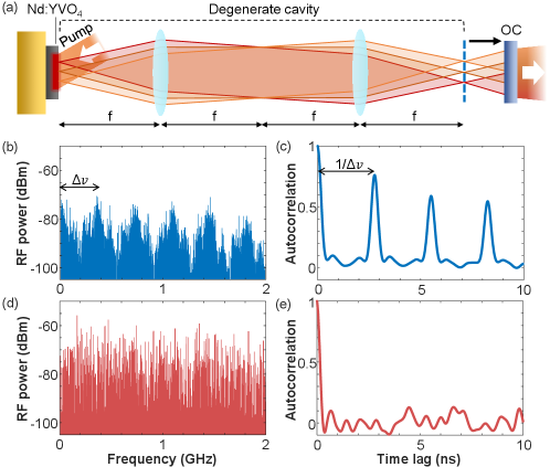
In principle, the degenerate cavity has the self-imaging property, where any point on one end mirror is imaged back onto itself after light propagates one round trip inside the cavity [Fig. 1(a)]. This property, combined with optical pumping, allows simultaneous lasing in many transverse modes with degenerate frequency and quality factor arnaud1969degenerate ; pole1965conjugate . Each transverse mode creates a diffraction-limited area on the gain disk, and the total number of lasing modes is given by the ratio of the pump area over the diffraction area. The latter is determined by the numerical aperture of the cavity as well as optical misalignment. Small misalignments, aberrations, and thermal lensing induce a small degree of inherent detuning Arnaud69p2 , therefore in practice the frequency degeneracy is slightly lifted with limited spectral spread.
Continuous-wave lasing is achieved in the degenerate cavity with optical pumping at room temperature. The pump beam has a diameter of 2 mm on the gain disk. The optical pump power is 22 W, well above the lasing threshold of 4.1 W. The output emission power from the degenerate cavity is 1.1 W. Since the optical gain bandwidth ( GHz) is much wider than the frequency spacing of longitudinal modes (free spectral range = 0.375 GHz), lasing occurs for hundreds of longitudinal modal groups, each containing many near-degenerate transverse modes chriki2018spatiotemporal .
The beating of transverse and longitudinal lasing modes creates intensity variations in space and time. If the temporal fluctuation is random at each location and uncorrelated with other locations, these intensity traces can be used for parallel LiDAR via spatial multiplexing. We characterize the laser emission intensity fluctuation using an amplified InGaAs photodetector (Newport, 818-BB-30A, 1.5 GHz bandwidth) and a real-time high-speed oscilloscope (Keysight UXR0204A, 20 GHz bandwidth). We note that 1.5 GHz (20 GHz) is the minimum 3-dB bandwidth tabulated by the manufacturer, beyond which the signal is attenuated electrically (digitally). Fourier transform of the time trace of emission intensity gives the radio-frequency (RF) spectrum. Figure 1(b) shows the experimental RF spectrum of the nearly degenerate cavity laser, obtained by taking the Fourier magnitude squared . It features periodic modulation, with dominant RF components clustered around the integer multiples of . We also compute the temporal correlation of emission intensity, , where denotes averaging over time . In Fig. 1(c), exhibits a series of correlation peaks spaced by ns, which corresponds to the round-trip time in the cavity. Such long-range correlation reflects periodic oscillation of emission intensity, which will significantly degrade the performance of our random LiDAR.
To suppress the long-range correlation in time, we need to generate a flatter RF spectrum, which is also a key feature in chaotic LiDAR lin2004chaotic . This is achieved by further breaking the frequency degeneracy between different transverse lasing modes with cavity detuning mahler2021fast . As shown in Fig. 1(a), we slightly offset the axial location of the output coupler by about 1 cm. The transverse modes, represented by diffraction-limited spots at the original plane of the output coupler, will diffract and partially overlap at the new position. The spatial overlap leads to mode coupling, which lifts the frequency degeneracy. Temporal interference between these transverse modes will create additional beat notes that fill the gaps between integer multiples of in the RF spectrum [Fig. 1(d)]. Consequently, long-range temporal correlations are significantly reduced, as shown in Fig. 1(e). Hence, detuning the degenerate cavity geometry randomizes the temporal variation of laser intensity, which can be used for LiDAR.
III Axial resolution
The axial resolution of random LiDAR is determined by the time scale of intensity fluctuation, or the bandwidth of the RF spectrum. To investigate how broad the RF spectrum is for the detuned cavity, we replace the aforementioned amplified photodetector with one having an order-of-magnitude higher bandwidth (Newport, 818-BB-36, 22 GHz bandwidth) combined with a low-noise amplifier (AT Microwave, AT-LNA-0018-3825H, 38-dB gain). The far-field emission out of the laser cavity is collected and sampled by a real-time high-speed oscilloscope (Keysight UXR0204A, 20 GHz bandwidth) at a sampling rate of 128 GS/s.
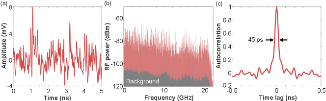
As shown in Fig 2(a), the measured emission intensity exhibits rapid random fluctuation in time. The RF spectrum in Fig. 2(b) features densely packed peaks caused by many-mode beating. Each peak has a narrow linewidth (5 kHz measured from 1 ms-long trace, frequency resolution of 1 kHz). The numerous peaks are distributed more or less uniformly over a broad range in the RF domain. These peaks have irregular spacings and varying amplitudes, constituting a broad, dense RF spectrum. The sharp drop at 20 GHz is due to the limited bandwidth of the oscilloscope.
The wide RF spectrum corresponds to a short time scale of emission intensity fluctuation. Figure 2(c) shows the temporal autocorrelation of intensity trace from the detuned degenerate cavity laser. The correlation width , defined by full-width-at-half-maximum (FWHM) of the temporal correlation function , is 45 ps. It determines the axial resolution of the random LiDAR, namely, two targets separated axially by a distance mm, can be resolved with ps.
The broad RF spectrum and fast temporal decorrelation of emission intensity from the detuned degenerate cavity laser will significantly improve the axial resolution of random LiDAR. The experimentally measured RF bandwidth and decorrelation time are still limited by the electrical bandwidth of our photodetection setup. The intrinsic RF spectrum width is dictated by the laser emission spectral width at optical frequency, which sets the largest beat notes (frequency difference) of lasing modes. We measure the optical spectrum of laser emission using a spectrometer with a wavelength resolution of 0.04 nm (Horiba TRIAX550 equipped with CCD3000, 1200 gr/mm). The wavelength width (FWHM) of the multimode laser emission is about 0.4 nm, corresponding to a frequency bandwidth of 100 GHz kim2021massively . With sufficiently fast photodetection, the ultimate axial resolution of our LiDAR can be about 1 mm, which exceeds that of chaotic LiDAR.
IV Spatial multiplexing
The number of spatial channels available for parallel random LiDAR is determined by the number of transverse lasing modes. To ensure a large number of transverse modes lasing, the detuning of the degenerate cavity is kept small, so that the reduction of quality factors for high-order transverse modes is less significant. The beating of many transverse and longitudinal lasing modes creates complex intensity fluctuations in space and time. The number of distinct random waveforms generated at different spatial locations can be used as separate channels for parallel LiDAR.
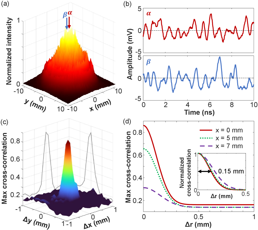
To find the number of uncorrelated time traces generated by the detuned degenerate cavity laser, we characterize the spatially-resolved temporal fluctuations of emission intensity. The laser beam profile at the output coupler is enlarged by a factor of 6.7 with a set of imaging optics. Figure 3(a) shows the emission intensity profile measured by a CCD camera (Allied Vision, Mako G-131B). The time-integrated output pattern is a superposition of many transverse lasing modes. The effective beam diameter, defined by FWHM of azimuthally-averaged intensity, is 9.8 mm. The central region with strong emission within this effective beam diameter will be investigated for parallel LiDAR.
To measure intensity fluctuations at different spatial locations simultaneously, we divide the output laser beam using a 50/50 beamsplitter and place two amplified InGaAs photodetectors (Newport, 818-BB-30A, 1.5 GHz bandwidth) at each arm. The two arms have an identical length so that the two photodetectors simultaneously measure the intensity fluctuations at different locations of the output beam. By varying the transverse positions of the two photodetectors, we obtain two time traces with different separations across the beam. Figure 3(b) shows temporal fluctuations of emission intensity at two locations with a transverse distance of 1 mm, denoted as and . The distinct time traces can be used as independent probes for parallel LiDAR.
To find how close two spatial channels can be, we characterize the spatial correlation of intensity fluctuations. For two transverse positions and , the cross-correlation of intensity fluctuations is given by . Experimentally, one photodetector is fixed in space, as the other one is scanned laterally across the output beam. For every offset , the maximal magnitude of among all time delay is plotted in Fig. 3(c). The maximal cross-correlation has the largest value when the lateral positions of two photodetectors coincide (). With increasing offset in the lateral position, the time traces become different, and the maximal correlation drops rapidly. Eventually, at a large offset, the maximal cross-correlation levels off to a constant value. We attribute this residual correlation to the finite number of beat notes in the RF spectrum.
The width of maximal cross-correlation sets the lateral width of a spatial channel of parallel LiDAR. Figure 3(d) shows the azimuthally averaged maximal cross-correlation as a function of radial distance . Each curve is fit by a Gaussian function with a constant background. The three curves represent the cross-correlations measured at different locations across the beam: at the center ( mm, ), at the effective beam radius ( mm, ), and near the beam edge ( mm, ). The peak value of correlation at decreases from the beam center to the edge, as the emission intensity gets weaker and the signal-to-noise ratio (SNR) becomes lower (10 dB, 4.5 dB, 2.3 dB for = 0, 5, 7 mm, respectively). To find the correlation width, we normalize the correlation functions in the inset of Fig. 3(d). The half-width-at-half-maximum (HWHM) increases from 0.15 mm at the beam center to 0.18 mm near the edge. The channel width , defined as twice the HWHM, varies from 0.3 mm to 0.36 mm across the beam. To have spatial channels with uncorrelated intensity fluctuations, we set the channel spacing to 0.6 mm. Given the effective beam diameter of 9.8 mm [Fig. 3(a)], the output beam of our single laser will provide approximately 300 independent spatial channels for parallel LiDAR.
V Isolating spatial channels
One issue for long-distance ranging is the mixing of spatial channels outside the laser cavity. Upon axial propagation, individual channels diffract and overlap with other channels in space. Their interference will make temporal intensity fluctuations vary with propagation distance. Consider a spatial channel at transverse location , its intensity trace at different longitudinal positions (along -axis) is not related simply by a temporal offset, i.e., , where is the speed of light. Instead, the temporal profile completely changes along .
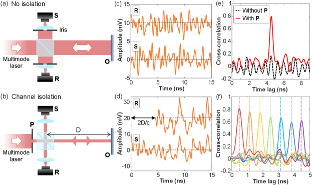
Typically for ranging applications, the reference beam of one channel propagates a much shorter distance to a detector than the probe beam reflected from an object. Their intensity traces would be uncorrelated, as confirmed experimentally below. A multimode laser beam is split to reference and probe beams by a beamsplitter [see Fig. 4(a)]. The reference beam is directed to a photodetector. An iris is placed in front of the lens to select a single spatial channel. The probe beam is reflected from a mirror and goes to a second detector. Another iris in front of the second lens selects the same spatial channel as the reference. The path length difference between the reference and probe beams is 1.35 m. Their intensity traces are completely different [Fig. 4(c)], and exhibit no cross-correlation peak at any time lag [black dashed curve in Fig. 4(e)]. This result indicates the temporal profile of intensity fluctuation in a single spatial channel becomes uncorrelated with free-space propagation, and thus cannot be used for ranging applications.
To resolve this issue, the spatial channels must be isolated to stop their beating outside the laser cavity. There are several methods of isolation. One is coupling the multimode laser emission into a fiber bundle by a lens array. The fields in individual single-mode fibers no longer couple, and the time traces of intensity remain invariant with propagation (except for a time lag). Another way is using a two-dimensional array of pinholes to isolate spatial channels. As a proof-of-concept demonstration, we filter a single spatial channel with a pinhole. Below we show its temporal profile remains invariant with axial propagation, and will use it for ranging.
Figure 4(b) is a schematic of our experimental LiDAR setup with an isolated spatial channel. The output beam from the detuned degenerate cavity laser is attenuated to 0.3 W. Then, to select a single spatial channel, in the beam we place a pinhole with 0.5 mm diameter, which is slightly smaller than the channel spacing of 0.6 mm. The power of this separated single channel is 0.36 mW. The filtered beam passes through a 50/50 beamsplitter to form the reference and the probe. The reference beam directly goes to a photodetector R. As an object for LiDAR demonstration, we use a flat aluminium mirror with a reflectivity of 85% at 1064 nm. The probe beam is reflected from the object and subsequently measured by a second photodetector S. To increase the collection efficiency, we use a plano-convex lens (focal length = 40 mm) to focus light onto the active area of the amplified photodetector (Newport, 818-BB-30A, 1.5 GHz bandwidth, 100 m diameter). The probe beam power (after the 50/50 beamsplitter) is 0.18 mW, well below the safety regulation limit (class-1 lasers, 2 mW for emission at 1064 nm) for commercial LiDAR applications dai2022requirements ; ansi2014laser .
Figure 4(d) shows the time traces measured by two photodetectors S and R. The signal trace S exhibits nearly identical intensity fluctuation as the reference R, except for an offset in time. The offset is given by , where is the distance from the beamsplitter to the object, as the distance from the beamsplitter to S is equal to that to R. The object distance can be retrieved from the cross-correlation between the signal and reference traces. Figure 4(e) shows a dominant peak of the cross-correlation (solid red curve) at the time lag corresponding to . Experimentally we move the object so that varies from 7 cm to 66 cm, corresponding to an interval from 0.46 ns to 4.4 ns time delay. For all distances, a cross-correlation peak stands out of the fluctuating background [Fig. 4(f)]. Its time lag gives the object distance , which agrees well with the actual distance (vertical lines).
VI Random LiDAR performance
We characterize the axial resolution of the ranging measurement. The resolution is a measure to distinguish two adjacent peaks, and thus determined by the peak width of the cross-correlation. From Fig. 4(f), the FWHM of the correlation peak ns yields the axial resolution = 5.3 cm. We note that the axial resolution is limited by the bandwidth of our photodetectors (1.5 GHz), and it can be improved with high-bandwidth photodetectors.
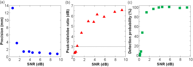
We further measure the precision and detection capability of our LiDAR. The target is a high-reflectivity Aluminium mirror (reflectivity of 85% at 1064 nm) placed at a distance = 30 cm. The sampling rate is 128 GS/s, and the time interval to compute cross-correlation is 200 ns. To characterize the LiDAR performance as a function of the SNR, we vary the signal strength by inserting neutral density filters into the beam path. To find the precision, we perform 100 consecutive ranging measurements and obtain statistics of the time lag for the maximal cross-correlation. Its standard deviation remains less than ps, which implies that the precision is = 1.5 mm, for SNR higher than 3 dB [Fig. 5(a)]. However, the precision quickly becomes worse, once the SNR falls below 3 dB.
The detection capability of LiDAR is characterized by the peak-sidelobe ratio, which indicates how strong the peak is compared to the background of cross-correlation. It is defined as the ratio between the maximal peak height and three times the standard deviation of the background. We measure the peak-sidelobe ratio for 100 consecutive measurements, and the averaged results are plotted as a function of SNR in Fig. 5(b). With SNR higher than 3 dB, the peak-sidelobe ratio remains larger than 5 dB, above the 3 dB limit for successful detection chen20213d .
Lastly, we investigate the detection probability [Fig. 5(c)]. We repeat the measurement one hundred times and examine whether the target can be detected. The detection probability is defined by the fraction of successful detection over the total number of measurements. The detection probability remains nearly 100% for the SNR higher than 4 dB. However, it rapidly drops at lower SNR.
VII Parallel LiDAR
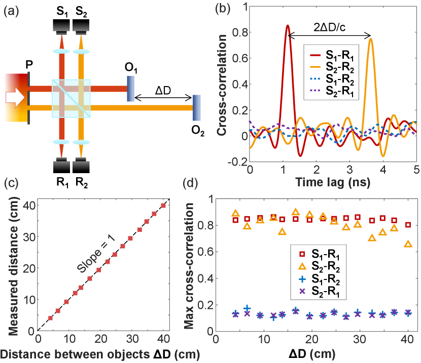
Next, we conduct simultaneous ranging of different targets using multiple spatial channels. As a proof-of-principle demonstration, we use two spatial channels. In order to generate two separate beams whose time traces are invariant with axial propagation, we use a double-pinhole mask to isolate two spatial channels [Fig. 6(a)]. Each pinhole diameter is 0.5 mm, and the edge-to-edge distance between the two pinholes is 2.0 mm. Since the double-pinhole mask is placed at the same plane where the spatial correlation function of laser emission in Fig. 3(d) is measured, the spatial correlation width of 0.3 mm is much smaller than the separation of two pinholes, and the intensity fluctuations in two filtered channels are uncorrelated. Both channels are split to reference and probe beams. Two targets (aluminum mirrors with a reflectivity of 85% at 1064 nm) are axially separated by 37 cm. Channel 1 (2) probes the first (second) target (), and the difference in propagation distance between signal and reference beams is cm ( cm). Both signal and reference of two spatial channels are measured simultaneously by four photodetectors (Newport, 818-BB-30A, bandwidth 1.5 GHz).
Figure 6(b) shows the cross-correlations between the same or different channels. Between the signal and the reference of the same channel ( and ), their cross-correlation clearly exhibits a peak. The peaks for the two channels are located at different time lags, as the distances to and are different. The spacing between two peaks is given by , where is the axial distance between two objects. Figure 6(b) reveals that is 37 cm, which matches the actual distance between and .
To show that our method can detect the objects with a wide range of distances, we vary by shifting one object axially, while keeping the other object fixed. Figure 6(c) shows that the measured distance agrees well with the actual distance.
Lastly, we verify that two spatial channels are uncorrelated. Figure 6(b) shows negligible cross-correlations between the signal and reference from different channels ( and ). This is further confirmed at a varying distance between two objects . As shown in Fig. 6(d), over a wide range of , the maximal cross-correlation for different channels remains low, while the maximal cross-correlation between signal and reference of the same channel is significantly higher. The absence of correlation between different spatial channels is a key to parallel random LiDAR.
VIII Robustness to interference
Finally, we investigate the anti-interference capability of our parallel random LiDAR. Interference may occur when multiple beams from different spatial channels overlap in space due to a long free-space propagation distance, which can degrade the ranging performance. We start with the simplest case of overlapping fields and from two spatial channels,
| (1) |
where and are field intensity of two channels, and represents their interference. For ranging with channel 1, the signal in Eq. (1) is cross-correlated with channel 1 reference [proportional to ]. Here and cause additional fluctuations in channel 1 signal. Since the interference term contains , it may lead to unwanted correlation with channel 1 reference .
We first experimentally investigate the interference of two spatial channels. Their respective probe beams, after being reflected from separate targets, become partially overlapped at the detector. In order to enhance their spatial overlap, we use two pinholes with 0.5 mm edge-to-edge distance to select two spatial channels, each pinhole diameter is still 0.5 mm. The experimental setup is modified from that of two-channel LiDAR in Fig. 6(a). The axial distance from the beamsplitter to object is 17 cm, and to object is 26 cm. Thus the two objects are separated axially by 9 cm. The two signal beams hit and separately. The reflected beams and diffract and partially overlap at a photodetector. The measured signal is a mixture of and .
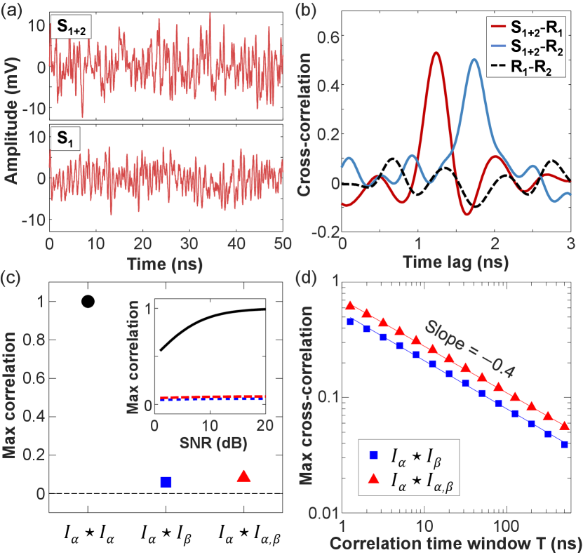
As shown in Fig. 7(a), the time trace of features a larger fluctuation amplitude than , which is the echo of with removed. The SNR of two mixed channels is 12 dB, while that for one channel is 9 dB, which are both far below the 33 dB SNR at the saturation limit of our photodetector. The difference between and is 3 dB, implying that the fluctuation power for is twice of that for . It indicates that the echoes and from two objects and are mixed with nearly identical amplitude of fluctuation.
Figure 7(b) shows cross-correlations between measured time traces. First of all, the two references and have negligible correlation, confirming the two spatial channels are uncorrelated. The mixed signal has correlation peaks with both references and , but at different time lags, which correspond to the axial distances of objects and . Hence, both objects are clearly distinguished despite the spatial overlap of their echoes.
To understand the experimental results, we numerically simulate cross-channel interference. A multimode laser beam is constructed by linear superposition of many transverse and longitudinal modes (see Appendix for details). The transverse mode frequencies are randomly distributed over the free spectral range. We choose 15 spatial channels at different positions , and compute the time trace of the optical field in each channel . From it, we calculate the intensity trace as well as its interference with another channel [see Eq. (1)]. The mean intensity is set to be identical for all channels. For every interference term , two channels and are mixed with equal amplitude.
We calculate the cross-correlation for every pair of spatial channels, and average the maximal cross-correlation over all possible pairs of 15 channels. The accumulation time for correlation is set to 200 ns, to be consistent with the experiment. Figure 7(c) shows that cross-correlation between different channels is close to zero, while autocorrelation of every channel is unity. Moreover, the correlation between the intensity trace of a single channel and its interference with another channel, , also vanishes. Hence, the interference between spatial channels does not create an additional peak in the correlation between signal () and reference () of the individual channel.
The channel interference effects diminish as a result of averaging correlation over a sufficient time interval . Even when the interference term has a comparable magnitude to the signal , its correlation with the reference decreases monotonically with increasing accumulation time . In Fig. 7(d), maximal correlations of both and decay with a similar slope in the double logarithmic scale.
The numerical results in Figs. 7(c,d) are obtained without noise, yet in real measurements the detection noise plays a significant role. Based on the measured noise of our photodetector, we simulate the detection noise with uncorrelated Gaussian intensity distribution. The inset of Fig. 7(c) shows that the noise has a notable impact on the autocorrelation (), which decreases with reducing SNR. The cross-correlation () and the interference term () are less affected by the noise, as they are already uncorrelated before adding the noise. The entire curves of maximal cross-correlation in Fig. 7(d) shift downward in the presence of noise but its slopes are unchanged (not shown).
When the number of overlapping channels is more than two, the mixed echo with equal contribution from channels is expressed as:
| (2) |
denotes an intensity sum of all channels except , and includes field interference terms among all channels. Correlating the mixed signal with channel reference produces three terms. The correlation peak of the first term gives the distance of an object probed by channel , and the second and third terms add fluctuating backgrounds to cross-correlation. Our numerical results reveal that the maximum of the second term scales as for , and the maximum of the third term scales as approximately . Both drop with accumulation time , making background correlations negligible for sufficiently long . Hence, our parallel LiDAR is robust to cross-channel interference.
IX Discussion and conclusion
In summary, we experimentally demonstrate parallel random LiDAR by utilizing spatiotemporal intensity fluctuations from a highly multimode laser. By detuning a degenerate cavity, we lift the frequency degeneracy of transverse modes without significant reduction of quality factors, so that lasing occurs in several hundreds of transverse modes simultaneously. Thanks to their frequency diversity, the spatio-temporal interference of all lasing modes creates numerous beat frequencies densely packed in the RF domain. The complex intensity fluctuations in space and time produce several hundreds of probe beams for parallel ranging. Our method does not need any optical modulator or external feedback. Instead, a single free-running laser can generate a large set of random waveforms in parallel. For the proof-of-concept demonstration, we have used an existing degenerate cavity laser of length 40 cm. For applications such as autonomous vehicles, robots, drones, compact size is essential, and our laser cavity length may be halved by placing a mirror at the cavity center, and further reduced to a few centimeters by using a lens of shorter focal length, while keeping the same number of transverse lasing modes. The output power of our degenerate cavity laser can reach 10 W with sufficient cooling liew2017intracavity . To further increase the power, a single multimode amplifier may be used to amplify the multimode laser emission.
To keep the temporal profiles of intensity fluctuations in individual spatial channels invariant with free-space propagation, we stop the spatio-temporal mode beating outside the laser cavity by isolating spatial channels with pinholes. The number of parallel spatial channels with uncorrelated intensity fluctuations is limited by the number of transverse lasing modes kim2021massively . We expect 300 spatial channels would be available from a single laser. In this proof-of-principle demonstration, we use only two spatial channels, but it will be straightforward to further increase the number of spatial channels by using a 2D array of pinholes or coupling the emission into a fiber bundle. collimated beams may be steered simultaneously by a single mechanical element for block scanning. Compared to the temporal or spectral multiplexing scheme which uses a single photodetector in the receiver, our spatial multiplexing scheme requires an array of photodetectors to measure the time traces of individual spatial channels simultaneously. Alternatively, a single photodetector may record the signals from multiple spatial channels, thanks to uncorrelated intensity fluctuations in different channels [Figs. 7(a,b)].
The broad and dense RF bandwidth of highly multimode laser emission enables a superior axial resolution of LiDAR. In our two-channel demonstration, the photodetectors have a bandwidth of 1.5 GHz, which limits the axial resolution to 5.3 cm. By using the 22-GHz bandwidth photodetector, the axial resolution can be further improved to 0.7 cm. The axial resolution is ultimately limited by the optical spectral bandwidth of the laser emission. Given the measured multimode emission bandwidth of 100 GHz, the axial resolution of our LiDAR can be as high as 1 mm. In practical situations of limited detection bandwidth, a narrowband spectral filter may be inserted into the degenerate cavity to reduce the laser emission linewidth in order to increase the detection efficiency.
We also demonstrate the robustness of our parallel ranging scheme to cross-channel interference. Although the mixing of signals from different spatial channels significantly changes the temporal profile of intensity fluctuations, cross-correlation with the reference of the individual channel can distinguish different targets. This is because the cross-channel interference terms have a negligible correlation with the intensity fluctuation of individual channels. Such anti-interference characteristics will be particularly useful in the presence of many-channel interference, making our method suitable for massively parallel LiDAR.
In addition to LiDAR, our scheme is applicable to parallel RADAR. Direct measurement of laser emission from a detuned degenerate cavity by a 2D array of photodiodes will generate distinct random waveforms to feed an array of antennas for spatially demultiplexed RADAR. Our scheme has advantages over other demultiplexing schemes of chaotic signals in radio-frequency cheng2015generation , optical frequency yao2015distributed ; lukashchuk2021chaotic ; lukashchuk2022chaotic , polarization zhong2017real ; zhong2021precise , and time domain chen20223 ; feng2022pulsed . Time-division demultiplexing inevitably requires a longer acquisition time for more channels, while for spatial demultiplexing the number of channels is independent of acquisition time. Compared to spectral demultiplexing, spatial demultiplexing is able to provide many channels without sacrificing the bandwidth and resolution of the individual channel. Moreover, our source has an intrinsic bandwidth of 100 GHz and can thus generate simultaneously several independent channels in various RF bands of interest for RADAR, such as the band (12-18 GHz), the band (27-40 GHz) and the band (75-110 GHz), where the last is not accessible with temporal chaos from semiconductor lasers under optical feedback lukin2022generation . Without those trade-offs, our parallel ranging scheme based on a high-power many-mode laser will facilitate high-speed 3D sensing and imaging.
Appendix: Numerical modeling
Multimode lasing
To simulate the laser beam in a detuned degenerate cavity, we calculate a linear superposition of many spatial modes with randomly distributed frequencies. Considering the cylindrical symmetry of the laser cavity, we choose Laguerre-Gaussian modes as the modal basis. The spatial profile of a Laguerre-Gaussian mode in a polar coordinate is given by siegman1986lasers ,
| (3) |
where and are the radial and azimuthal mode numbers, is the generalized Laguerre polynomial, and is the beam radius for the fundamental transverse mode. Every modal profile is normalized by . We sort the modes from low-order to high-order transverse modes in ascending order of , and label them by with the transverse mode index . For instance, correspond to of (0,0), (0,1), (0,-1), (1,0), (0,2), (0,-2), respectively.
A linear superposition of many transverse and longitudinal modes is expressed as:
| (4) |
where is the longitudinal mode index, is the resonant mode frequency, and is the random phase between 0 and . We sum over Laguerre-Gaussian transverse modes, and longitudinal modal groups. The lowest frequency is set by the emission wavelength 1064 nm. The free spectral range is given by 375 MHz.
To simulate the detuning of a degenerate cavity, we randomize the distribution of transverse mode frequencies. The spacing between adjacent transverse modes follows a uniform probability distribution between 0 and . The mean transverse mode spacing is set to , which makes the transverse modes almost uniformly distributed within one free spectral range.
After calculating the near-field profile , we extract 15 time traces at a normalized distance 2.9 from the cavity axis. These locations have the largest number of overlapping transverse modes, which leads to minimal long-range temporal correlations of intensity fluctuations. The time step of sampling is set to 20 ps. For Figs. 7(c-d), we average over 10 random distributions of mode frequencies.
Cross-correlation
We first normalize the field at every channel such that the variance of the intensity fluctuation becomes unity, i.e. , where is the intensity time trace. The maximal cross-correlation between two intensity time traces and are then calculated as,
| (5) |
where … is the average within the time window of length . The cross-correlation with any other intensity trace [, , and of the main text] is also calculated by Eq. (5) but with replaced by .
The intensity time trace of noise is simulated by the independent Gaussian distribution, with the mean 0 and the standard deviation , where is the SNR in decibels. It is added to the intensity trace of signal , and the variance of the intensity fluctuation is normalized before plugging into Eq. 5.
Acknowledgement
We acknowledge funding from US Naval Office of Research under Grant No. N00014-221-1-2026.
References
- (1) B. Schwarz, “Mapping the world in 3D,” Nat. Photonics 4, 429–430 (2010).
- (2) M.-C. Amann, T. M. Bosch, M. Lescure, R. A. Myllylae, and M. Rioux, “Laser ranging: a critical review of usual techniques for distance measurement,” Opt. Eng. 40, 10–19 (2001).
- (3) I. Kim, R. J. Martins, J. Jang, T. Badloe, S. Khadir, H.-Y. Jung, H. Kim, J. Kim, P. Genevet, and J. Rho, “Nanophotonics for light detection and ranging technology,” Nat. Nanotechnol. 16, 508–524 (2021).
- (4) D. Wang, C. Watkins, and H. Xie, “MEMS mirrors for LiDAR: a review,” Micromachines 11, 456 (2020).
- (5) E. Fishler, A. Haimovich, R. Blum, D. Chizhik, L. Cimini, and R. Valenzuela, “Mimo radar: An idea whose time has come,” in Proceedings of the 2004 IEEE Radar Conference (IEEE Cat. No. 04CH37509), (IEEE, 2004), pp. 71–78.
- (6) Y. Jiang, S. Karpf, and B. Jalali, “Time-stretch LiDAR as a spectrally scanned time-of-flight ranging camera,” Nat. Photonics 14, 14–18 (2020).
- (7) J. Riemensberger, A. Lukashchuk, M. Karpov, W. Weng, E. Lucas, J. Liu, and T. J. Kippenberg, “Massively parallel coherent laser ranging using a soliton microcomb,” Nature 581, 164–170 (2020).
- (8) A. Lukashchuk, J. Riemensberger, A. Tusnin, J. Liu, and T. Kippenberg, “Chaotic micro-comb based parallel ranging,” arXiv:2112.10241 (2021).
- (9) J.-D. Chen, K.-W. Wu, H.-L. Ho, C.-T. Lee, and F.-Y. Lin, multi-input multi-output (MIMO) pulsed chaos lidar based on time-division multiplexing, IEEE J. Sel. Top. Quantum Electron. 28, 1–9 (2022).
- (10) Z. Zang, Z. Li, Y. Luo, Y. Han, H. Li, X. Liu, and H. Fu, “Ultrafast parallel single-pixel LiDAR with all-optical spectro-temporal encoding,” APL Photonics 7, 046102 (2022).
- (11) R. Chen, H. Shu, B. Shen, L. Chang, W. Xie, W. Liao, Z. Tao, J. E. Bowers, and X. Wang, “Breaking the temporal and frequency congestion of lidar by parallel chaos,” Nat. Photonics pp. 1–9, (2023).
- (12) M. E. Warren, D. Podva, P. Dacha, M. K. Block, C. J. Helms, J. Maynard, and R. F. Carson, “Low-divergence high-power VCSEL arrays for lidar application,” in Vertical-Cavity Surface-Emitting Lasers XXII, vol. 10552 (SPIE, 2018), pp. 72–81.
- (13) M. Dummer, K. Johnson, S. Rothwell, K. Tatah, and M. Hibbs-Brenner, “The role of VCSELs in 3D sensing and lidar,” in Optical Interconnects XXI, vol. 11692 (SPIE, 2021), pp. 42–55.
- (14) N. Takeuchi, N. Sugimoto, H. Baba, and K. Sakurai, “Random modulation cw lidar,” Appl. Opt. 22, 1382–1386 (1983).
- (15) C. Nagasawa, M. Abo, H. Yamamoto, and O. Uchino, “Random modulation cw lidar using new random sequence,” Appl. Opt. 29, 1466–1470 (1990).
- (16) M. Bashkansky, H. Burris, E. Funk, R. Mahon, and C. Moore, “RF phase-coded random-modulation LIDAR,” Opt. Commun. 231, 93–98 (2004).
- (17) R. Matthey and V. Mitev, “Pseudo-random noise-continuous-wave laser radar for surface and cloud measurements,” Opt. Lasers Eng. 43, 557–571 (2005).
- (18) X. Ai, R. Nock, J. G. Rarity, and N. Dahnoun, “High-resolution random-modulation cw lidar,” Appl. Opt. 50, 4478–4488 (2011).
- (19) L. Feng, H. Gao, J. Zhang, M. Yu, X. Chen, W. Hu, and L. Yi, “FPGA-based digital chaotic anti-interference lidar system,” Opt. Express 29, 719–728 (2021).
- (20) J. T. Spollard, L. E. Roberts, C. S. Sambridge, K. McKenzie, and D. A. Shaddock, “Mitigation of phase noise and doppler-induced frequency offsets in coherent random amplitude modulated continuous-wave lidar,” Opt. Express 29, 9060–9083 (2021).
- (21) C. S. Sambridge, J. T. Spollard, A. J. Sutton, K. McKenzie, and L. E. Roberts, “Detection statistics for coherent RMCW LiDAR,” Opt. Express 29, 25945–25959 (2021).
- (22) Y. Chen, Y. Xie, C. Liu, and L. Chen, “Investigation of anti-interference characteristics of frequency-hopping LiDAR,” IEEE Photon. Technol. Lett. 33, 1443–1446 (2021).
- (23) L. Guosui, G. Hong, and S. Weimin, “Development of random signal radars,” IEEE Trans. Aerosp. Electron. Syst. 35, 770–777 (1999).
- (24) X. Xu and R. M. Narayanan, “Range sidelobe suppression technique for coherent ultra wide-band random noise radar imaging,” IEEE Trans. Antennas Propag. 49, 1836–1842 (2001).
- (25) F.-Y. Lin and J.-M. Liu, “Chaotic radar using nonlinear laser dynamics,” IEEE J. Quantum Electron. 40, 815–820 (2004).
- (26) L. Wang, Y. Guo, P. Li, T. Zhao, Y. Wang, and A. Wang, “White-chaos radar with enhanced range resolution and anti-jamming capability,” IEEE Photon. Technol. Lett. 29, 1723–1726 (2017).
- (27) K. Myneni, T. A. Barr, B. R. Reed, S. D. Pethel, and N. J. Corron, “High-precision ranging using a chaotic laser pulse train,” Appl. Phys. Lett. 78, 1496–1498 (2001).
- (28) F.-Y. Lin and J.-M. Liu, “Chaotic lidar,” IEEE J. Sel. Top. Quantum Electron. 10, 991–997 (2004).
- (29) J. Ohtsubo, Semiconductor lasers: stability, instability and chaos, vol. 111 (Springer, 2012).
- (30) J. Zhu, X. Chen, P. Huang, and G. Zeng, “Thermal-light-based ranging using second-order coherence,” Appl. Opt. 51, 4885–4890 (2012).
- (31) C.-M. Tsai and Y.-C. Liu, “Anti-interference single-photon LiDAR using stochastic pulse position modulation,” Opt. Lett. 45, 439–442 (2020).
- (32) I.-P. Hwang and C.-H. Lee, “Mutual interferences of a true-random LiDAR with other lidar signals,” IEEE Access 8, 124123–124133 (2020).
- (33) C.-H. Cheng, C.-Y. Chen, J.-D. Chen, D.-K. Pan, K.-T. Ting, and F.-Y. Lin, “3D pulsed chaos lidar system,” Opt. Express 26, 12230–12241 (2018).
- (34) J.-D. Chen, H.-L. Ho, H.-L. Tsay, Y.-L. Lee, C.-A. Yang, K.-W. Wu, J.-L. Sun, D.-J. Tsai, and F.-Y. Lin, “3D chaos lidar system with a pulsed master oscillator power amplifier scheme,” Opt. Express 29, 27871–27881 (2021).
- (35) H.-L. Ho, J.-D. Chen, C.-A. Yang, C.-C. Liu, C.-T. Lee, Y.-H. Lai, and F.-Y. Lin, “High-speed 3D imaging using a chaos lidar system,” Eur. Phys. J.: Spec. Top. 231, 435–441 (2022).
- (36) H.-L. Tsay, C.-H. Chang, and F.-Y. Lin, “Random-modulated pulse lidar using a gain-switched semiconductor laser with a delayed self-homodyne interferometer,” Opt. Express 31, 2013–2028 (2023).
- (37) M. Nixon, B. Redding, A. Friesem, H. Cao, and N. Davidson, “Efficient method for controlling the spatial coherence of a laser,” Opt. Lett. 38, 3858–3861 (2013).
- (38) S. F. Liew, S. Knitter, S. Weiler, J. F. Monjardin-Lopez, M. Ramme, B. Redding, M. A. Choma, and H. Cao, “Intracavity frequency-doubled degenerate laser,” Opt. Lett. 42, 411–414 (2017).
- (39) J. Arnaud, “Degenerate optical cavities,” Appl. Opt. 8, 189–196 (1969).
- (40) R. Pole, “Conjugate-concentric laser resonator,” J. Opt. Soc. Am. 55, 254–260 (1965).
- (41) J. A. Arnaud, “Degenerate optical cavities. ii: Effect of misalignments,” Appl. Opt. 8, 1909–1917 (1969).
- (42) R. Chriki, S. Mahler, C. Tradonsky, V. Pal, A. A. Friesem, and N. Davidson, “Spatiotemporal supermodes: Rapid reduction of spatial coherence in highly multimode lasers,” Phys. Rev. A 98, 023812 (2018).
- (43) S. Mahler, Y. Eliezer, H. Yılmaz, A. A. Friesem, N. Davidson, and H. Cao, “Fast laser speckle suppression with an intracavity diffuser,” Nanophotonics 10, 129–136 (2021).
- (44) Z. Dai, A. Wolf, P.-P. Ley, T. Glück, M. C. Sundermeier, and R. Lachmayer, “Requirements for automotive lidar systems,” Sensors 22, 7532 (2022).
- (45) American National Standards Institute, ANSI Z136. 1-2014 Laser Safety Standard for the Safe Use of Lasers (Laser Institute of America, 2014).
- (46) K. Kim, S. Bittner, Y. Zeng, S. Guazzotti, O. Hess, Q. J. Wang, and H. Cao, “Massively parallel ultrafast random bit generation with a chip-scale laser,” Science 371, 948–952 (2021).
- (47) C.-H. Cheng, Y.-C. Chen, and F.-Y. Lin, “Generation of uncorrelated multichannel chaos by electrical heterodyning for multiple-input–multiple-output chaos radar application,” IEEE Photonics J. 8, 1–14 (2015).
- (48) T. Yao, D. Zhu, D. Ben, and S. Pan, “Distributed MIMO chaotic radar based on wavelength-division multiplexing technology,” Opt. Lett. 40, 1631–1634 (2015).
- (49) A. Lukashchuk, J. Riemensberger, A. Stroganov, G. Navickaite, and T. J. Kippenberg, “Chaotic microcomb inertia-free parallel ranging,” arXiv:2212.14275 (2022).
- (50) D. Zhong, G. Xu, W. Luo, and Z. Xiao, “Real-time multi-target ranging based on chaotic polarization laser radars in the drive-response VCSELs,” Opt. Express 25, 21684–21704 (2017).
- (51) D. Zhong, N. Zeng, H. Yang, Z. Xu, Y. Hu, and K. Zhao, “Precise ranging for the multi-region by using multi-beam chaotic polarization components in the multiple parallel optically pumped spin-VCSELs with optical injection,” Opt. Express 29, 7809–7824 (2021).
- (52) W. Feng, N. Jiang, Y. Zhang, J. Jin, A. Zhao, S. Liu, and K. Qiu, “Pulsed-chaos mimo radar based on a single flat-spectrum and delta-like autocorrelation optical chaos source,” Opt. Express 30, 4782–4792 (2022).
- (53) K. Lukin, O. Zemlyanyi, and S. Lukin, “Generation of chaotic and random signals for noise radar-brief overview,” in 2022 23rd International Radar Symposium (IRS), (IEEE, 2022), pp. 163–168.
- (54) A. E. Siegman, Lasers (University science books, 1986).