Parallelizing Over Artificial Neural Network Training Runs with Multigrid
Abstract
Artificial neural networks are a popular and effective machine learning technique. Great progress has been made on speeding up the expensive training phase of a neural networks, leading to highly specialized pieces of hardware, many based on GPU-type architectures, and more concurrent algorithms such as synthetic gradients. However, the training phase continues to be a bottleneck, where the training data must be processed serially over thousands of individual training runs. This work considers a multigrid reduction in time (MGRIT) algorithm that is able to parallelize over the thousands of training runs and converge to the same solution as traditional serial training. MGRIT was originally developed to provide parallelism for time evolution problems that serially step through a finite number of time-steps. This work recasts the training of a neural network similarly, treating neural network training as an evolution equation that evolves the network weights from one step to the next. Thus, this work concerns distributed computing approaches for neural networks, but is distinct from other approaches which seek to parallelize only over individual training runs. The work concludes with supporting numerical results that demonstrate feasibility for two model problems.
1 Introduction
Artificial neural networks are a popular and effective machine learning technique (see [4] for a general introduction). Great progress has been made on speeding up the expensive training phase of an individual network, leading to highly specialized pieces of hardware, many based on GPU-type architectures, and more concurrent algorithms such as synthetic gradients. However, the training phase continues to be a bottleneck, where the training data must be processed serially over thousands of individual training runs, thus leading to long training times. This situation is only exacerbated by recent computer architecture trends where clock speeds are stagnant, and future speedups are available only through increased concurrency.
This situation repeats itself for the time-dependent PDE simulation community, where it has been identified as a sequential time-stepping bottleneck [6]. In response, interest in parallel-in-time methods, that can parallelize over the time domain, has grown considerably in the last decade. One of the most well known parallel-in-time methods is Parareal [13], which is equivalent to a two-level multigrid method [9]. This work focuses on the multilevel approach, multigrid reduction in time (MGRIT) [6]. MGRIT uses coarser representations of the problem to accelerate the solution on the finest level. The coarse level equations provide coarse level error corrections to the finest level and are complemented by a fine-scale relaxation process that corrects fine-scale errors. The multilevel nature of MGRIT gives the algorithm optimal parallel communication behavior and an optimal number of operations, in contrast to a two-level scheme, where the size of the second level limits parallelism and optimality. For a good introduction to the history of parallel-in-time methods, see the recent review paper [8].
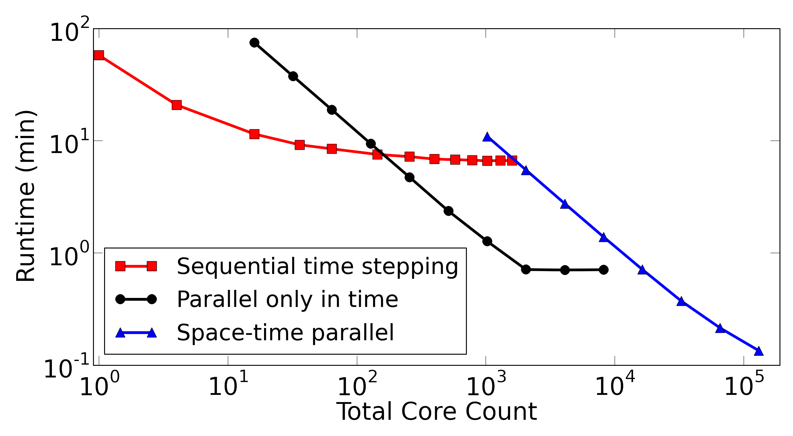
The power of parallel-in-time methods can be seen in Figure 1. Here, a strong scaling study for the linear diffusion problem is carried out on the machine Vulcan (IBM BG/Q) at Lawrence Livermore. (See [16].) Sequential time-stepping is compared with two processor decompositions of MGRIT, a time-only parallel MGRIT run and a space-time parallel MGRIT run using 64 processors in space and all other processors in time. The maximum possible speedup is approximately 50, and the cross-over point is about 128 processors, after which MGRIT provides a speedup.
Two important properties of MGRIT are the following. One, MGRIT is able to parallelize over thousands of training runs and also converge to the exact same solution as traditional sequential training. MGRIT does this by recasting the training of a neural network as an evolution process that evolves the network weights from one step to the next, in a process analogous to time-steps. Thus, this work concerns distributed computing approaches for neural networks, but is distinct from other approaches which seek to parallelize only over individual training runs. The second property is that MGRIT is nonintrusive. The evolution operator is user-defined, and is often an existing sequential code that is wrapped within the MGRIT framework. MGRIT is not completely agnostic to the user’s problem; however, in that the convergence of the method is problem dependent. Nonetheless, the approach developed here could be easily applied to other existing implementations of serial neural network training.
Parallelizing over the time dimension and even over the steps of a general evolutionary process can seem surprising at first, but the feasibility of this approach has been shown. For instance, MGRIT has already been successfully used in the non-PDE setting for powergrid problems [11]. In fact, it can be natural to think of neural network training as a time-dependent process. For instance, a network is trained by “viewing” consecutive sets of images. In the biological world, this would certainly be happening in a time-dependent way, and the computer-based approximations to these networks can also be thought of as stepping through time, as training runs are processed. More precisely, if the training of a network with weights is represented by a function application , traditional serial training of the network can be described as
| (1) |
where is a vector of the weight values at training step , represents the evolution of these weights to step , and is the total number of training runs. Other researchers have made similar an analogies between a training run and a time-step [10, 14].
Thus, the goal here is to parallelize over these consecutive applications, as MGRIT has already parallelized over time-steps in other settings, e.g. for Navier-Stokes [7] and nonlinear parabolic problems [16]. The resulting MGRIT algorithm will converge to the same solution as that obtained from a traditional sequential processing of the training runs.
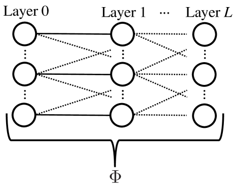
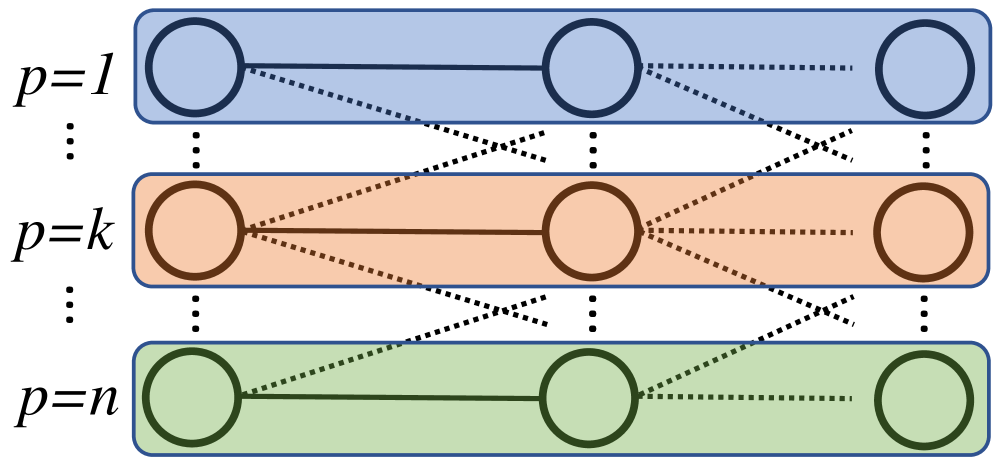
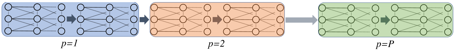
Figure 2(b) depicts the proposed form of parallelism over applications, and compares it to other types of possible parallelism. Figure 2(a) provides a reference figure for a single application. Figure 2(b) depicts parallelism inside of a single application, where the problem is decomposed across processors (denoted “”), and each processor owns some slice of the nodes. (While the number of nodes is usually not constant across layers, we ignore that here simply for the purpose of having a straight-forward pictorial representation). Figure 2(c) depicts parallelism inside of a single application, where the layers are decomposed across the processors. Finally, Figure 2(d) depicts parallelism where entire applications are decomposed across processors, which is the approach pursued here. Each processor owns two applications, but this is not fixed.111These types of parallelism could be mixed, as has been done for PDE-based problems in [6, 5], but the scope of this paper is on approach in Figure 2(d).
As motivation for MGRIT, consider a simple thought experiment for a two-level MGRIT approach to training. Let the fine level contain 100 training runs, and the coarse level contain 50 training runs. MGRIT will use the coarse level only to accelerate convergence on the fine level by computing error corrections on the coarse level. It is reasonable to consider the possibility that a 50 training run example could provide a good error correction to a 100 training run example. MGRIT will do this in a multilevel way, so that the 50 training run example is never solved exactly, thus avoiding sequential bottlenecks.
The challenge of developing strategies for good MGRIT convergence for our model neural network problems allows this paper to make some novel achievements. To the best of our knowledge, this is the first successful application of parallel-in-time techniques to neural networks. To do this, we develop some novel MGRIT strategies such using the learning rate in a way similar to time-step sizes. We also explore serializing over all training examples, to allow for more potential parallelism.
In Section 2, we introduce our first model neural network, the MGRIT algorithm, and some motivation for designing an MGRIT solver for neural network training. In Section 3, we develop the proposed MGRIT approach, apply it to two model problems, and compute maximum possible speedup estimates. In Section 4, concluding remarks are made.
2 Motivation
In this section, we first formalize our notation for MGRIT and the example neural networks, and then conclude with motivation for the proposed method.
2.1 Model Neural Network
To define a multilayer network, we let there be nodes on level and weights connecting level to level . In general, a superscript [⋅] will denote a level in the neural network, not MGRIT level. We say that there are in total weights in the network. Indexing always starts at 0.
For the model problems considered here, the networks are fully connected that is each node on level has a weight connecting it to every node on level . Thus, we skip any further notation defining the edges (connections) in the network. While we assume a fixed network topology for each example, we note that adaptive network topologies (e.g., adding and removing weights) could be integrated into our solver framework (see [5]) by using strategies researched for MGRIT in the classical PDE setting.
Our simplest neural network model problem is based on the three-layer example from [18]. This network is trained to learned an exclusive OR (XOR) operation, where the th training input is and the th expected output is , i.e.,
| (2) | ||||
The single hidden layer has four nodes, yielding an input layer of , the hidden layer of , and a single output node of . The total number of weights is (). The threshold function is a standard sigmoid,
| (3) |
and standard backpropagation [17, 12, 15] is used to train the network. The strategy is that MGRIT must first be effective for such simple model problems, before it is reasonable to experiment with larger problems.
The serial training code for this network is from [18] and reproduced in Appendix A for convenience. However, we briefly review the general process of network training for readability. First, the forward propagation evaluates the network by initializing the input nodes to values from the th training instance . Then these node values are used in a matrix-vector multiply with the matrix representing the weights connecting layers 0 and 1. Then the threshold function is applied element-wise to the result vector of size . This procedure of matrix-vector multiply and threshold evaluation continues across all the hidden layers, until values at the output nodes are obtained. The initial gradient is then obtained by differencing with the value(s) at the output layer. This gradient is then propagated backwards, updating the weights between each level. The size of the step taken in the gradient direction is called the learning rate .
The proposed MGRIT algorithm will provide the same solution as this sequential training process, to withing some tolerance. Later, we will apply MGRIT to a larger, four-layer problem.
2.2 MGRIT
The description of MGRIT also requires some notation and nomenclature. Let the from equation (1) be the propagator or evolution operator that trains the network. One training run is a single application. Each training run is functionally equivalent to a time-step in the traditional MGRIT framework. Thus, we will call a training run a “training step” from now on, to emphasize the connection between time-dependent evolution problems and the training of artificial neural networks.
The th training step has a corresponding training data set called . For the above example in Section 2.1, we define
| (4) |
Thus, is the same for all here, and the network does a batch training on all four training instances simultaneously (although we will explore variations on this later).
In conclusion, one application is equivalent to a forward propagation of the training data in with , followed by a backpropagation step that creates the updated set of weights . When done sequentially over all training steps, equation (1) is obtained.
However, the serial training process can also be represented as a global operator with block rows, representing the training steps. To do this we “flatten” each set of weights so that becomes a vector of length . This global operator of size is
| (5) |
where equals the initial values assigned to the weights by the user. A forward solve using forward substitution of this equation is equivalent to the traditional serial training of a neural network. Instead, MGRIT solves equation (5) iteratively, with multigrid reduction, allowing for parallelism over the training steps. That is, all training steps are computed simultaneously. Being an iterative method, the proposed approach also converges to the exact same solution as that produced by traditional serial training. MGRIT accomplishes this by constructing a hierarchy of training levels. Each coarse level provides an error correction to the next finer level in order to accelerate convergence on that level. Complementing these error corrections is a local relaxation process that resolves fine-scale behavior.
Regarding complexity, both serial propagation and MGRIT are methods, but MGRIT is highly parallel.222MGRIT is when it converges in a scalable way, with a fixed iteration count regardless of problem size. On the other hand, the computational constant for MGRIT is higher, generally leading to a cross-over point, where beyond a certain problem size and processor count, MGRIT offers a speedup (see Figure 1).
2.3 MGRIT Algorithm
We will first describe MGRIT for linear problems, and then describe the straight-forward extension to nonlinear problems. The description is for a two-level algorithm, but the multilevel variant is easily obtained through recursion.
We denote as the number of training steps on level 0, which is the finest level that defines the problem to be solved, and as the problem size on level . In general, a superscript (⋅) will hereafter denote a level in the MGRIT hierarchy, and a subscript will denote a training step number. If the subscript denoting a training step number is omitted, the quantity is assumed to be constant over all training steps on that level.
2.3.1 MGRIT for Linear Problems
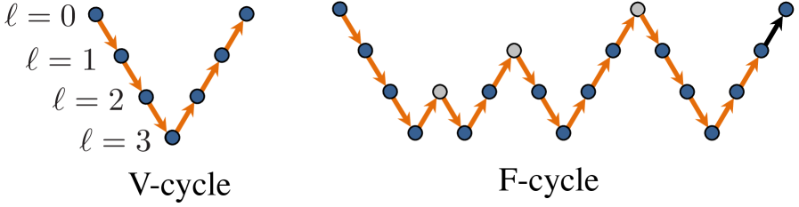
MGRIT solves an evolution problem over a finite number of evolution steps. For time-dependent PDEs, these steps correspond to time-steps. For a more general evolution problem, these steps need not be PDE-based. Regardless, MGRIT defines a fine level and coarse level of evolution steps, based on the coarsening factor . (Here, we use a level independent coarsening factor.) There are steps on level 0 and for level 1. Two such levels for are depicted in Figure 3.333For time-dependent PDEs, these levels represent a fine and coarse time step spacing, respectively, with the fine time-step size four times smaller than the coarse level time-step size. Typical values for are 2, 4, 8, and 16.
Multigrid reduction is similar to an approximate block cyclic reduction strategy, and similarly eliminates block rows and columns in the system (5). If all the block rows corresponding to the black fine points in Figure 3 are eliminated from the system (5), then using the level notation (level 1 is coarse, and level 0 is fine), the coarse system becomes
| (6) |
where represents the th power, i.e., consecutive applications of . Here, we assume that is the same function over all training steps for simplicity, although the method extends easily to the case where depends on the training step number. The operator represents “Ideal” restriction and we also define an interpolation , as in [6],
| (7a) | ||||
| (7b) | ||||
The operator injects coarse points from the coarse- to fine-level, and then extends those values to fine-points with a application. This will be equivalent to injection, followed by F-relaxation (defined below).
The operator can be formed in a typical multigrid fashion with , and we refer to this as the ideal coarse-level operator because the solution to (6) yields the exact fine-level solution at the coarse points.444The ideal coarse-level operator can also be obtained with the injection operator , . For efficiency, we therefore will use injection later on in the algorithm. The interpolation is also ideal, and uses to compute the exact solution at the fine points. However, this exact solution process is in general as expensive as solving the original fine-level problem, because of the applications in . MGRIT “fixes” this issue by approximating with , i.e.,
| (8) |
where is an approximation of . One obvious choice here is to approximate with , i.e., approximate training steps with one training step. For time-dependent PDEs, is usually a single time-step using a larger time-step size that approximates finer time-steps. How well approximates will govern how fast MGRIT converges, and choosing a that allows for fast convergence is typically the main topic of research for a given problem area.
Thus, the two-level algorithm uses the coarse level to compute an error correction based on the fine-level residual, , mapped to the coarse level with (see Step 2 in Algorithm 1). Complementing the coarse level correction is a local relaxation process on the fine-level which resolves fine-scale behavior. Figure 4 (from [16]) depicts F- and C-relaxation on a level with . F-relaxation updates the solution at each F-point by propagating the solution forward from the nearest coarse point (C-point). And, C-relaxation updates every C-point with a solution propagation from the nearest F-point. Overall, relaxation is highly parallel, with each interval of F-points being independently updated during F-relaxation, and likewise for C-relaxation. The nonintrusiveness of MGRIT is also apparent because the internals of are opaque to MGRIT. Thus, this approach can be easily applied by wrapping existing code bases.
2.3.2 Nonlinear Algorithm
The above two-level process can be easily to nonlinear problems using full approximation storage (FAS), a nonlinear multigrid scheme [1, 7].555We mention that the F-relaxation two-level MGRIT algorithm is equivalent to the popular parallel-in-time Parareal algorithm [9]. The key addition of FAS to the multigrid process is how the coarse-level equation is Step 3 is computed.
The two-level FAS version of MGRIT is described in Algorithm 1 (taken from [7]). A recursive application of the algorithm at Step 4 makes the method multilevel. This can be done recursively until a trivially sized level is reached, which is then solved sequentially. Ideal interpolation (7) is represented as two steps (5 and 6). Initial values for the weights can in principle be anything, even random values, which is the choice made here for as the initial condition. For all other points, is the initial value.
Multigrid solves can use a variety of cycling strategies. Here, we consider V- and F-cycles, as depicted in Figure 5, which shows the order in which levels are traversed. The algorithm continues to cycle until the convergence check based on the fine level residual is satisfied in line 6.
2.4 Motivation
The motivation for the proposed approach is based on similarities between neural network training and time-dependent evolution problems. We have already shown that the sequential neural network training approach of equation (1) can represented as a global system (5) solvable by MGRIT. However, the similarity goes even further, because we can represent any operator so that it resembles a forward Euler time-step.
| (9) |
where represents the computation of the gradient, i.e., the search direction for this update, and represents the length of the search step. (See lines 45–47 in Appendix A.) But, the parameter also resembles a time-step size, which could be varied in a level-dependent manner inside of MGRIT. This will be a key insight required for good MGRIT performance.
The other motivation is based on the fact that both the forward and backward phases of neural network training resemble discretized hyperbolic PDEs, which typically have an upper or lower triangular matrix form. If the neural network training algorithm were a purely linear process, then the forward phase would look like a block lower-triangular matrix-vector multiply, where the th block-row is the size of the th layer. And the backward phase, would be analogously upper block-triangular. Thus, we will consider solver strategies from [20] which considered MGRIT for hyperbolic PDEs. These strategies are slow coarsening (i.e., small values), FCF-relaxation (as apposed to F-relaxation), and F-cycles.
3 Method
In this section, we formalize how we describe an MGRIT solver for artificial neural networks. We must define , or the propagator on level for training step . This corresponds to block row in equation (5). We first define a “Naive Solver”, because it is the simplest, out-of-the-box option. Next, we will explore modifications that lead to faster convergence.
3.1 Naive Solver
To define , three chief subcomponents must be defined. For the Naive Solver, we choose the following.
Coarsening factor :
The coarsening factor , defines the problem size on each level. For example, , implies that . For the Naive Solver, we coarsen by a factor of 2. This yields a sequence of problems sizes on each level, of
Learning rate :
The learning rate on level is defined by . For the Naive Solver, we choose a fixed learning rate over all levels defined by a base learning rate , i.e.,
| (10) |
Training set :
The training set at level and training step is . For the examples considered here,
| (11) |
where is the input for the network, and is the desired output. For the Naive Solver will contain all of the training data, and is fixed, not changing relative to or . The data set and will contain four rows, and this training data will be processed in a standard “batch” manner for neural networks (see Appendix A). In other words, each application of will train over all of the training data. However, we will consider other options later, such as serializing over the training data.
Thus, we can say that is defined by
| (12) |
and that
| (13) |
where represent vectors of the weights defining the network.
3.2 Results
For our results we will experiment using FCF-relaxation and compare V-cycles, F-cycles and two-level solvers, while experimenting with various definitions. The maximum coarsest level size is 10 training steps, and the halting tolerance is . We scale the halting tolerance in a manner similar to PDE applications, so that the tolerance grows commensurately with problem size. The maximum number of iterations is 50, thus results that took longer are denoted as “50+” with a corresponding average convergence rate of “*”. The average convergence rate is computed as a geometric average, . The quantity is the residual from equation (5) after the MGRIT iterations, and the norm is the standard Euclidean norm.
Experimental Goal:
The goal of these experiments is to examine various MGRIT solvers, using heuristics to choose . A successful MGRIT solver will converge quickly, in say 10 or 15 iterations, and show little to no growth in iteration counts as the problem size increases. (Remember, MGRIT is an iterative algorithm, which updates the solution until the convergence check based on the fine level residual is satisfied in line 6 of Algorithm 1.) Such a result will be said to be “scalable” or “nearly scalable”, because the operation count required to solve equation (5) will be growing linearly with problem size. In parallel, however, there will always be a log-growth in communication related to the number of levels in the solver. For a good introduction to multigrid and the notion of scalability, see [2].
While two-level solvers are impractical, we will first examine them (as is typical for multigrid methods research). If success cannot be obtained in this simplified setting, there is little hope that a multilevel version of the solver will perform better.
3.3 Naive Solver Results
Using the Naive Solver from Section 3.1, in a two-level setting, yields the results in Table 1. The learning rate is , taken from from [18]. While convergence is poor, this result shows that MGRIT can converge for the problem in question.
| 100 | 200 | 400 | 800 | 1600 | 3200 | 6400 | 12800 | 25600 | |
|---|---|---|---|---|---|---|---|---|---|
| Iters | 14 | 19 | 24 | 31 | 40 | 49 | 50+ | 50+ | 50+ |
| 0.31 | 0.43 | 0.48 | 0.59 | 0.66 | 0.72 | * | * | * |
3.4 Improvements to Naive
3.4.1 Increasing
In this section, we consider the motivation in Section 2.4, and consider increasing on coarser levels. In particular, we consider doubling so that . Remarkably, this single change to the Naive Solver yields fast, scalable two-level iteration counts.
| 100 | 200 | 400 | 800 | 1600 | 3200 | 6400 | 12800 | 25600 | |
| Iters | 6 | 6 | 6 | 6 | 6 | 6 | 6 | 6 | 5 |
| 0.10 | 0.10 | 0.10 | 0.10 | 0.09 | 0.09 | 0.08 | 0.08 | 0.07 |
More generally, we consider defining as
| (14) |
where is some experimentally determined maximum stable value.666This connection between the size of and stability (i.e., values that do not diverge over multiple applications) shows another similarity between and time-step size. Here, , i.e., is allowed to increase up to level . Beyond that point, the training becomes “unstable”, and can no longer increase. While the halt to increasing values may negatively impact the algorithm, this halt occurs only on coarser levels, and so its negative impact on MGRIT convergence will hopefully be somewhat mitigated.
We denote this as Solver 1, which uses equation (14) to define , and equation (11) to define as containing all the training data. Together with and , this fully defines the method explored in this section.
Table 3 depicts the results for Solver 1. Initially the results look scalable (i.e., flat iteration counts and stable convergence rates ). But, eventually a log-type growth in the iterations becomes apparent. A possible culprit is the fact that is capped and cannot continually increase. V-cycle results are quite poor and hence omitted for brevity.
| 100 | 200 | 400 | 800 | 1600 | 3200 | 6400 | 12800 | 25600 | |
| Iters | 6 | 6 | 7 | 7 | 7 | 8 | 11 | 16 | 21 |
| 0.10 | 0.10 | 0.09 | 0.10 | 0.09 | 0.07 | 0.17 | 0.24 | 0.34 |
One important parameter that affects the MGRIT convergence rate is the base learning rate . Decreasing this value improves the MGRIT convergence rate, while also requiring more training steps to adequately train the network. Exploration of this trade-off is future research, but we make note of it here. If we take Solver 1, decrease from 1.0 to 0.5 and keep , we get the improved F-cycle iterations in Table 4
| 100 | 200 | 400 | 800 | 1600 | 3200 | 6400 | 12800 | 25600 | |
| Iters | 5 | 5 | 5 | 6 | 6 | 5 | 6 | 9 | 12 |
| 0.07 | 0.08 | 0.08 | 0.06 | 0.05 | 0.04 | 0.05 | 0.07 | 0.18 |
3.4.2 Serializing the Training Data
In this section, we note that there is unutilized parallelism in the method. All four training examples are processed simultaneously as a “batch”. That is, is defined by an and with four rows, representing the four training sets (see equation (11). Instead, each of the four training sets can be broken up and processed individually, resulting in four times as many possible steps to parallelize. More precisely, for training instances, define and to correspond to the mod-th training instance.
Here , so would train the network with the first training data set with . would train the network for the second training data set with , and so on. Once the training step index passes the value , the process repeats, so that again trains on the first training data set with . This strategy exposes significantly more parallelism than the “unserialized” .
We denote this as Solver 2, which defines
| (15) |
Solver 2 continues using equation (14) to define and . Together with and , this fully defines the method explored in this section.
Table 5 depicts two-level results using Solver 2, which show a scalable convergence rate, but the rate is slower than that in Table 2 for Solver 1.
| 100 | 200 | 400 | 800 | 1600 | 3200 | 6400 | 12800 | 25600 | |
| Iters | 10 | 12 | 15 | 18 | 20 | 20 | 20 | 20 | 19 |
| 0.18 | 0.23 | 0.28 | 0.36 | 0.40 | 0.39 | 0.39 | 0.38 | 0.38 |
However, Table 6 depicts Solver 2 results for F-cycles, and this shows an unscalable increase in iteration counts.
| 100 | 200 | 400 | 800 | 1600 | 3200 | 6400 | 12800 | 25600 | |
| Iters | 10 | 12 | 15 | 21 | 26 | 27 | 29 | 41 | 50 |
| 0.18 | 0.23 | 0.29 | 0.40 | 0.47 | 0.47 | 0.50 | 0.60 | 0.99 |
One possible contributing factor the unscalable iteration growth in Table 6 is the fact that is allowed to only grow on the first four levels. To investigate this possibility, Table 7 runs the same experiment as in Table 6, but with with and . We see that this combination of a smaller base , which allows to grow up to level dramatically improves the scalability of the F-cycles. The downside is the smaller learning rate. We leave a further investigation of this for future work, because a deeper theoretical understanding is required to meaningfully guide our tests.
| 100 | 200 | 400 | 800 | 1600 | 3200 | 6400 | 12800 | 25600 | |
| Iters | 5 | 5 | 5 | 6 | 7 | 8 | 10 | 13 | 14 |
| 0.05 | 0.06 | 0.07 | 0.11 | 0.10 | 0.14 | 0.15 | 0.25 | 0.24 |
Remark 1
The reader will note that this strategy of serializing the training data is independent of . For example, MGRIT interpolation and restriction connects point on level 1 to point on level 0. However, this serialized training set definition defines the training instance on level 1 for point as mod and on level 0 for point as mod. The values mod mod, in general. Experiments were run where the training instances on level 0 were injected to all coarser levels, to avoid this discrepancy, but this approach lead to worse convergence. It is hypothesized that this is the case because the complete elimination of training instances on the coarser levels leads to poor spectral equivalence between coarse and fine . To address this, experiments were also run where coarse training sets represented averages of fine-level training sets, and this improved convergence, but not enough to compete with the above approach, even in a two-level setting. The averaging was done such that was the average of and , i.e., the average of the corresponding C- and F-point on level 0.
3.4.3 Potential Speedup
While the proposed method does allow for parallelism over training steps, we need to quantify possible parallel speedups for the proposed approach. To do that, we use a simple computational model that counts the dominant sequential component of the MGRIT process and compares that to the dominant sequential component of the traditional serial training approach. The dominant sequential component in both cases is the required number of consecutive applications, because this is the main computational kernel.
For sequential time stepping, the number of consecutive applications is simply . However for MGRIT, we must count the number of consecutive applications as the method traverses levels. Consider a single level during a V-cycle with a coarsening factor of 2. FCF-relaxation contains 3 sequential applications, the sweeps over F- then C- then F-points. Additionally, each level must compute an FAS residual (see Algorithm 1), which requires two matrix-vector products. In parallel at the strong scaling limit, each process in time will own two block rows that will likely be processed sequentially, resulting in 4 total sequential applications for the computation of the two matrix-vector products. Last, on all levels, but level 0, there is an additional application to fill in values at F-points for the interpolation. The coarsest level is an exception and only carries out a sequential solve no longer than the maximum allowed coarsest level size (here 10).
Taken together, this results in 7 sequential applications on level 0, and 8 on all coarser levels, except the coarsest level which has approximately 10. Thus, the dominant sequential component for a V-cycle is modeled as
| (16) |
where niter is the number of MGRIT iterations, or V-cycles, required for convergence.
The dominant sequential component of an F-cycle is essentially the concatenation of successive V-cycles starting on ever finer levels (see Figure 5), i.e.,
| (17) |
The reader will note that there is no final V-cycle done on level 0 in equation (17).
Thus, we define the potential speedup for V-cycles as and for F-cycles. This is a useful speedup measure, but it measures speedup relative to an equivalent sequential training run. For example, for the case of the double applications, this measure will compute a speedup against a sequential run that also does a double application.
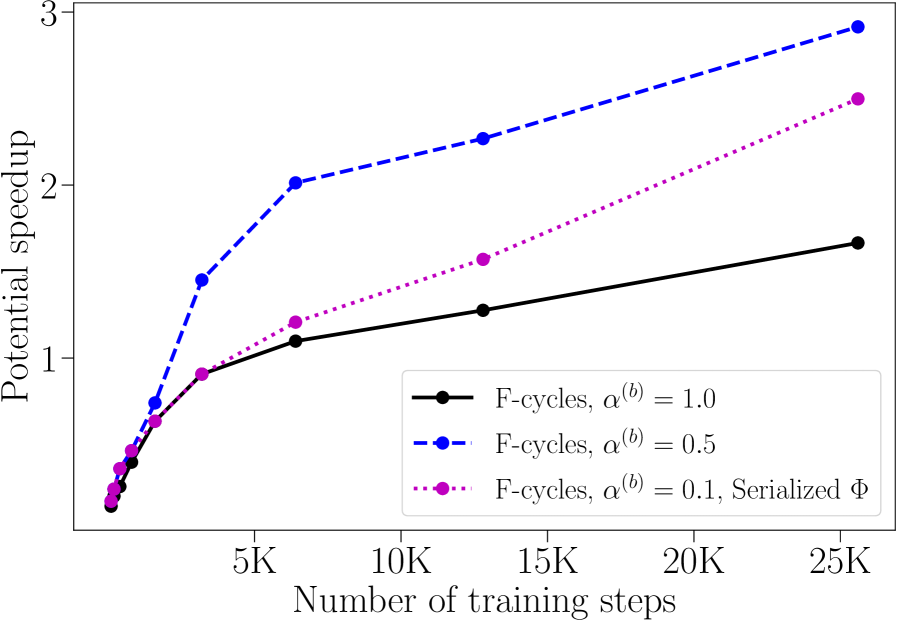
Figure 6 depicts the potential speedup for Solver 1 from Tables 3, 4 and Solver 3 from Table 7. Although this is a simple model problem, these results indicate that the observed convergence behavior offers promise for a useful speedup on more real-world examples. Also, the trend lines indicate that larger problem sizes would offer improved potential speedups.
Remark 2
We note that these speedup estimates are promising, there is much room for improvement. This paper represents an initial work meant to show feasibility of the approach. Future research will focus on improving the potential speedup, by for instance, considering coarsening the network on coarse levels, where the accuracy requirements of the training steps are reduced. Such approaches have lead to significant speedup improvements for PDEs, and are expected to do so here. Moreover, there is existing work [3] on transferring a network’s content between different sized networks.
Remark 3
The computed potential speedup here assumes that the problem has access to as much parallelism as needed. For training steps on level , that means having processors available. If fewer processors are available, then the potential speedup would be reduced.
3.5 Larger Example
In this section, we will investigate a larger example using the solvers developed above for the small, three-layer model problem.
In particular, we will examine a four-layer network with total weights. The training data is a synthetic dataset for binary addition created using a random number generator. The network takes two random binary numbers (12 bits in length) and then computes the 12 bit binary sum. The error produced by the network is the difference between the computed and actual sum. The network is fully connected with an input layer of nodes (12 for each binary number), first hidden layer of nodes, second hidden layer of nodes and an output layer of nodes. Note, . This example is based on Section 4 from [19], where the code of the serial training algorithm is as the “Plain Vanilla” algorithm based on backpropagation. The same sigmoid threshold function as in Section 2.1 is used.
We begin our experiments with the Naive Solver, using the from [19]. Remember for the Naive Solver, is defined to contain all the training data sets, which here means is defined as 500 pairs of random 12 bit numbers and then corresponds to the sum of those 500 pairs.
Table 8 depicts the two-level results for the Naive Solver. The results show some promise, but also large unscalable growth in iteration counts.
| 40 | 80 | 160 | 320 | 640 | 1280 | |
| Iters | 9 | 13 | 19 | 36 | 48 | 50 |
| 0.14 | 0.27 | 0.38 | 0.63 | 0.69 | 0.88 |
Following the direction of Section 3.4.1, we apply Solver 1, which increases on coarse-levels. We continue to use and set (based on experiments). Table 9 depicts these two-level Solver 1 results, which indicate some stability issues for , because the convergence rate is over 1.0.
| 40 | 80 | 160 | 320 | 640 | 1280 | |
| Iters | 9 | 50 | 50 | 50 | 50 | 50 |
| 0.13 | 1.01 | 1.02 | 1.02 | 1.02 | 1.02 |
Thus, we experiment with a smaller . Taking the Naive Solver, but changing to , yields the results depicted in Table 10.
| 40 | 80 | 160 | 320 | 640 | 1280 | |
| Iters | 8 | 12 | 17 | 23 | 31 | 43 |
| 0.11 | 0.24 | 0.37 | 0.49 | 0.61 | 0.70 |
Again following the direction of Section 3.4.1, we take this smaller and experiment with it in the context of Solver 1, continuing to use . Table 11 depicts these results, but again, we see unscalable iteration growth. There is a difficulty here for MGRIT that was not present for the three-layer example.
| 40 | 80 | 160 | 320 | 640 | 1280 | |
| Iters | 5 | 7 | 11 | 16 | 25 | 37 |
| 0.06 | 0.12 | 0.23 | 0.36 | 0.53 | 0.63 |
3.6 A Better Solver
To design a better solver, we begin by simply trying to understand which problem trait(s) make the performance of MGRIT differ to that observed for the small three-layer problem.
One key difference is the number of training examples. Here, the network is trained on 500 examples, while before for the three-layer example, only 4 examples were used. Thus, we take Solver 1 with and , but cut to contain only 50 training examples. Using this modified Solver 1 we get the results depicted in Table 12. The reduction in training examples has restored scalable iteration counts.
| 100 | 200 | 400 | 800 | 1600 | 3200 | 6400 | 12800 | |
| Iters | 4 | 5 | 7 | 11 | 14 | 13 | 14 | 14 |
| 0.04 | 0.07 | 0.15 | 0.27 | 0.35 | 0.37 | 0.39 | 0.39 |
The use of 50 training set examples is not an attractive approach, because it limits the ability to train a network. However, it does indicate potential promise for serializing over the training set data as in Section 3.4.2. We explore this idea in the next section.
3.6.1 Serialized Training Sets
In this section, we experiment with Solver 2, which serializes over the training data, and continue to use and . In other words, the first 500 training steps will train over the first 500 training data sets; training step 501 will loop back to the first training data set; and so on. Because of the smaller training data set size per step, we are able to run out to larger problem sizes.
Table 13 depicts two-level results for Solver 2. The iteration counts are good, but not quite scalable, showing some growth.
| 100 | 200 | 400 | 800 | 1600 | 3200 | 6400 | 12800 | |
| Iters | 4 | 4 | 5 | 5 | 6 | 6 | 7 | 11 |
| 0.05 | 0.07 | 0.07 | 0.09 | 0.10 | 0.13 | 0.18 | 0.29 |
Table 14 depicts F-cycle results for Solver 2. They are also not scalable, showing a slow growth, but the iteration counts are modest enough to potentially be useful. Table 15 depicts results for Solver 2 for V-cycles. The deterioration for larger problem sizes and F-cycles in Table 14 is visible when compared to the two-level results in Table 13. To investigate possible remedies, we again explore the possibility of allowing to grow on more levels. Table 16 carries out such a experiment, except this time we compute with
| (18) |
as opposed to equation (14), which uses powers of 2. This allows to grow on all levels for all experiments. The F-cycle results now show no deterioration from the two-level results in Table 13 for the large problem sizes. Unfortunately, this choice of did not show a significant improvement for V-cycles. We leave a further investigation of optimal coarse level as future work, because a deeper theoretical understanding is required to meaningfully guide our tests.
| 100 | 200 | 400 | 800 | 1600 | 3200 | 6400 | 12800 | |
| Iters | 4 | 4 | 5 | 5 | 6 | 6 | 8 | 13 |
| 0.05 | 0.07 | 0.07 | 0.09 | 0.10 | 0.13 | 0.17 | 0.34 |
| 100 | 200 | 400 | 800 | 1600 | 3200 | 6400 | 12800 | |
| Iters | 4 | 5 | 6 | 7 | 8 | 9 | 11 | 20 |
| 0.05 | 0.08 | 0.10 | 0.13 | 0.17 | 0.20 | 0.28 | 0.47 |
| 100 | 200 | 400 | 800 | 1600 | 3200 | 6400 | 12800 | |
| Iters | 4 | 4 | 4 | 5 | 6 | 6 | 7 | 10 |
| 0.04 | 0.06 | 0.07 | 0.08 | 0.09 | 0.12 | 0.14 | 0.27 |
Remark 4
Further reducing the factor of increase from 1.25 in equation (18) is not an option. If we revert to the naive strategy of fixing to be on all levels for Solver 2, even the two-level solver shows unscalable iteration counts. While we omit these results for brevity, we note that the key insight of increasing on coarse levels continues to be critical.
3.7 Potential Speedup
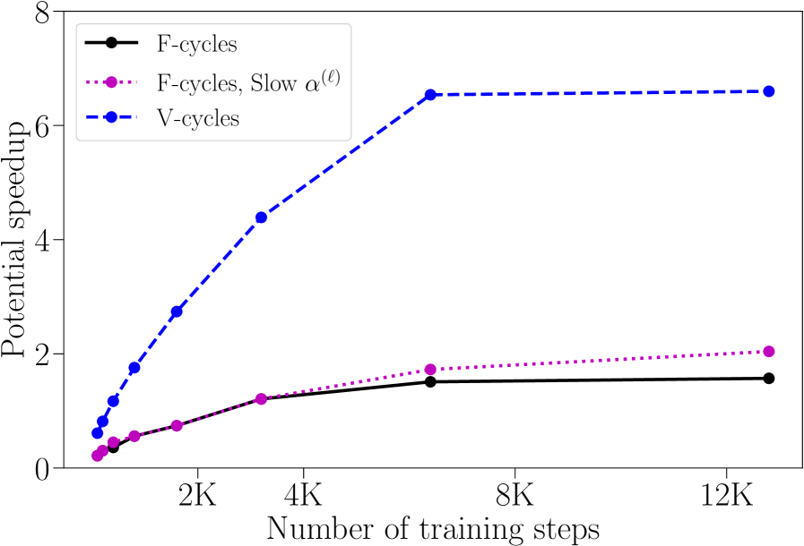
Figure 7 depicts the potential speedup for Solver 2 using Tables 15 and 14, respectively. The addition of another layer and many more weights to the network has not significantly impacted the possibility for speedup when compared to the three-layer example (see Section 3.4.3). We note that there is an unexplained deterioration in V-cycle convergence for the final data point. Also, the trend lines indicate that larger problem sizes would offer improved potential speedups.
4 Conclusion
We have shown a method that is able to parallelize over training steps (i.e., training runs) for artificial neural networks and also converge to the exact same solution as that found by traditional sequential training algorithms. To the best of our knowledge, this is the first successful application of such parallel-in-time techniques to neural networks.
The method relies on a multigrid reduction technique to construct a hierarchy of levels, where each level contains a fraction of the training steps found on the preceding level. The coarse levels serve to accelerate the solution on the finest level. The strategies developed here will hopefully lay the groundwork for application to more real-world applications later.
The chief challenge faced is the definition of the coarse-level propagator . Proposed solutions for constructing such coarse-level are treating the learning rate in a way similar to time-step sizes and using double applications of to provide for more effective MGRIT relaxation. We also explored serializing over all training examples, to allow for more potential parallelism. Solver 3 was the most robust, and the results indicate that MGRIT is able to offer a large possible speedup for the considered model problems.
Future research will focus on examining more challenging neural networks and on improving the potential speedup (See Remark 2). Another path for improving speedup is the development of a deeper theoretical understanding of this approach. This will help, for example, in choosing and designing . Here, we will look to leverage the existing MGRIT theory in [20].
References
- [1] A. Brandt, Multi–level adaptive solutions to boundary–value problems, Math. Comp., 31 (1977), pp. 333–390.
- [2] W. L. Briggs, V. E. Henson, and S. F. McCormick, A multigrid tutorial, SIAM, Philadelphia, PA, USA, 2nd ed., 2000.
- [3] T. Chen, I. Goodfellow, and J. Shlens, Net2net: Accelerating learning via knowledge transfer, arXiv preprint arXiv:1511.05641, (2015).
- [4] H. B. Demuth, M. H. Beale, O. De Jess, and M. T. Hagan, Neural network design, Martin Hagan, 2014.
- [5] R. D. Falgout, T. A. M. andJ. B. Schroder, and B. Southworth, Parallel-in-time for moving meshes, Tech. Rep. LLNL-TR-681918, Lawrence Livermore National Laboratory, 2016.
- [6] R. D. Falgout, S. Friedhoff, T. V. Kolev, S. P. MacLachlan, and J. B. Schroder, Parallel time integration with multigrid, SIAM J. Sci. Comput., 36 (2014), pp. C635–C661. LLNL-JRNL-645325.
- [7] R. D. Falgout, A. Katz, T. V. Kolev, J. B. Schroder, A. Wissink, and U. M. Yang, Parallel time integration with multigrid reduction for a compressible fluid dynamics application, Tech. Rep. LLNL-JRNL-663416, Lawrence Livermore National Laboratory, 2015.
- [8] M. J. Gander, 50 years of time parallel time integration, in Multiple Shooting and Time Domain Decomposition, T. Carraro, M. Geiger, S. Körkel, and R. Rannacher, eds., Springer, 2015, pp. 69–114.
- [9] M. J. Gander and S. Vandewalle, Analysis of the parareal time-parallel time-integration method, SIAM J. Sci. Comput., 29 (2007), pp. 556–578.
- [10] J. J. Hopfield, Neural networks and physical systems with emergent collective computational abilities, Proceedings of the national academy of sciences, 79 (1982), pp. 2554–2558.
- [11] M. Lecouvez, R. D. Falgout, C. S. Woodward, and P. Top, A parallel multigrid reduction in time method for power systems, Power and Energy Society General Meeting (PESGM), (2016), pp. 1–5.
- [12] Y. LeCun, Une procédure d’apprentissage pour réseau a seuil asymmetrique (a learning scheme for asymmetric threshold networks), in Proceedings of Cognitiva 85, Paris, France, 1985.
- [13] J. L. Lions, Y. Maday, and G. Turinici, Résolution d’EDP par un schéma en temps pararéel, C.R.Acad Sci. Paris Sér. I Math, 332 (2001), pp. 661–668.
- [14] R. Lippmann, An introduction to computing with neural nets, IEEE Assp magazine, 4 (1987), pp. 4–22.
- [15] D. B. Parker, Learning-logic: Casting the cortex of the human brain in silicon, Tech. Rep. Technical Report TR-47, Center for Computational Research in Economics and Management Science, MIT, Cambridge, MA, 1985.
- [16] B. O. R.D. Falgout, T.A. Manteuffel and J. Schroder, Multigrid reduction in time for nonlinear parabolic problems: A case study, SIAM J. Sci. Comput. (to appear), (2016). LLNL-JRNL-692258.
- [17] D. E. Rumelhart, G. E. Hinton, and R. J. Williams, Learning internal representations by error propagation, tech. rep., California Univ San Diego La Jolla Inst for Cognitive Science, 1985.
- [18] A. Trask, A neural network in 11 lines of python. http://iamtrask.github.io/2015/07/12/basic-python-network.
- [19] , Tutorial: Deepmind’s synthetic gradients. https://iamtrask.github.io/2017/03/21/synthetic-gradients.
- [20] N. P. V. Dobrev, Tz. Kolev and J. Schroder, Two-level convergence theory for multigrid reduction in time (mgrit), SIAM J. Sci. Comput. (to appear), (2016). LLNL-JRNL-692418.
Appendix A Code for Three-Layer Problem
As an aide to the reader, we reproduce the serial training algorithm (taken directly from [18]) that we base the three-layer model problem on from Section 2.1. The code is in Python.