Parameter Estimation and Adaptive Solution of the Leray-Burgers Equation using Physics-Informed Neural Networks
Abstract
This study presents a unified framework that integrates physics-informed neural networks (PINNs) to address both the inverse and forward problems of the one-dimensional Leray-Burgers equation. First, we investigate the inverse problem by empirically determining the characteristic wavelength parameter at which the Leray-Burgers solutions closely approximate those of the inviscid Burgers equation. Through PINN-based computational experiments on inviscid Burgers data, we identify a physically consistent range for being between 0.01 and 0.05 for continuous initial conditions and between 0.01 and 0.03 for discontinuous profiles, demonstrating the dependence of on initial data. Next, we solve the forward problem using a PINN architecture where is dynamically optimized during training via a dedicated subnetwork, Alpha2Net. Crucially, Alpha2Net enforces to remain within the inverse problem-derived bounds, ensuring physical fidelity while jointly optimizing network parameters (weights and biases). This integrated approach effectively captures complex dynamics, such as shock and rarefaction waves. This study also highlights the effectiveness and efficiency of the Leray-Burgers equation in real practical problems, specifically Traffic State Estimation.
1 Introduction
In this study, we explore the one-dimensional Leray-Burgers (LB) equation (2.1), a regularized model of the inviscid Burgers equation, which introduces a wavelength parameter to prevent finite-time blow-ups while aiming to preserve the essential dynamics of the inviscid case, such as shock waves. However, selecting an appropriate is a non-trivial task, as its value significantly influences the fidelity of the LB solutions to those of the inviscid Burgers equation. To address this challenge, we employ Physics-Informed Neural Networks (PINNs) [15, 14] in a two-step process that bridges the inverse and forward problems.
First, we tackle the inverse problem, empirically determining the range of that aligns LB solutions with inviscid Burgers entropy solutions under various initial conditions (Section 4). We find that the choice of depends on the initial data. For continuous initial profiles, the practical range of is –, whereas for discontinuous initial profiles, it is – (4.2). This step establishes a critical foundation by identifying the bounds within which yields physically meaningful results.
Next, we turn to the forward inference problem in Section 5 , where PINNs are utilized to solve the LB equation under different initial and boundary conditions. Unlike traditional approaches where might be arbitrarily fixed, we treat as a learnable parameter depending on , optimized during training alongside the standard PINN parameters (weights and biases). This optimization is facilitated by a dedicated subnetwork, Alpha2Net, integrated into the PINN architecture. To ensure that trained remains physically relevant, Alpha2Net constrains its values to the range determined from the inverse problem. This constraint links the two problems directly: the inverse problem informs the forward inference by providing a predetermined range that guides the optimization process, ensuring that the resulting solutions are accurate and consistent with the physical insights gained earlier.
We also apply the LB equation to a traffic state estimation to highlight the effectiveness and efficiency of the LB equation in real practical problems in Section 6. We present a brief investigation of two variants of the Lighthill-Whitham-Richards (LWR) traffic flow model, namely LWR- (based on the Leray-Burgers equation) and LWR- (based on the viscous Burgers equation), in the context of Traffic State Estimation (TSE). The result demonstrates the efficacy of the LWR- model as a suitable alternative for traffic state estimation, outperforming the diffusion-based LWR- model in terms of computational efficiency.
2 Background
2.1 Leray-Burgers Equation
We consider a problem of computing the solution of an evolution equation
| (2.1) | ||||
where is a nonlinear differential operator acting on with a small constant parameter ,
| (2.2) |
Here, the subscripts of mean partial derivatives in and , is a bounded domain, denotes the final time and is the prescribed initial data. Although the methodology allows for different types of boundary conditions, we restrict our discussion to Dirichlet or periodic cases and prescribe the boundary data as
where denotes the boundary of the domain .
Equation (2.1) is called the Leray-Burgers equation (LB). It is also known as Burgers-, connectively filtered Burgers equation, Leray regularized reduced order model, etc., in literature. Bhat and Fetecau [2] introduced (2.1) as a regularized approximation to the inviscid Burgers equation
| (2.3) |
They considered a special smoothing kernel associated with the Green function of the Helmholtz operator
where is interpreted as the characteristic wavelength scale below which the smaller physical phenomena are averaged out (see, for example, [8]) and it accelerates energy decay. Applying the smoothing kernel to the convective term in (2.3) yields
| (2.4) |
where is a vector field and is the filtered vector field. The filtered vector is smoother than and the equation (2.4) is a nonlinear Leray-type regularization [12] of the inviscid Burgers equation. Here and in the following, we abuse the notation of the filtered vector with . If we express the equation (2.4) in the filtered vector , it becomes a quasilinear evolution equation that consists of the inviscid Burgers equation plus nonlinear terms [2, 3, 4]:
| (2.5) |
In this paper, we follow Zhao and Mohseni [21] to expand the inverse Helmholz operator in to higher orders of the Laplacian operator:
where is the highest eigenvalue of the discretized operator . Then we can write (2.4) in the unfiltered vector fields to obtain the equation (2.1)-(2.2) with truncation error.
For smooth initial data that decrease at least at one point (so there exists such that ), the classical solution of the inviscid Burgers equation (when ) fails to exist beyond a specific finite break time . It is because the characteristics of the inviscid equation intersect in finite time. The Leray-Burgers equation bends the characteristics to make them not intersect each other, avoiding any finite-time intersection and remedying the finite-time breakdown [2, 4]. So, the Leray-Burgers equation possesses a classical solution globally in time for smooth initial data for [2]:
Theorem 1.
Given initial data , the Leray-Burgers equation (2.4) possesses a unique solution for all .
Furthermore, the Leray-Burgers solution with initial data for converges strongly, as , to a global weak solution of the following initial value problem for the inviscid Burgers equation (Theorem 2 in [2]):
Bhat and Fetecau [2] found numerical evidence that the chosen weak solution in the zero- limit satisfies the Oleinik entropy inequality, making the solution physically appropriate. The proof relies on uniform estimates of the unfiltered velocity rather than the filtered velocity . It made possible the strong convergence of the Leray-Burgers solution to the correct entropy solution of the inviscid Burgers equation. In the context of the filtered velocity , they also showed that the Leray-Burgers equation captures the correct shock solution of the inviscid Burgers equation for Riemann data consisting of a single decreasing jump [4]. However, since captures an unphysical solution for Riemann data comprised of a single increasing jump, it was necessary to control the behavior of the regularized equation by introducing an arbitrary mollification of the Riemann data to capture the correct rarefaction solution of the inviscid Burgers equation. With that modification, they extended the existence results to the case of discontinuous initial data . However, it is still an open problem for the initial data . In [7], Guelmame, et all, derived a similar regularized equation to (2.5):
| (2.6) |
which has an additional term on the right-handed side. Notice that in this equation is the filtered vector field in (2.4). When they were establishing the existence of the entropy solution, Guelmame, et all. resorted to altering the equation (2.6), as Bhat and Fetecau had to modify the initial data for their proof in [4]. Analysis in the context of the filtered vector field appears to induce an additional modification of the equations to achieve the desired results. Working with the actual vector field may avoid such arbitrary changes.
Equation (2.4) and related models have previously appeared in the literature. We refer [1, 2, 3, 4, 6, 7, 11, 13, 17, 20, 18] for more properties related to the Leray-Burgers equation. The paper [17] explores the role of in regularizing Proper Orthogonal Decomposition (POD)-Galerkin models for the Kuramoto-Sivashinsky (KS) equation. The -regularization is introduced to enhance the stability and accuracy of these models by applying Helmholtz filtering to the eigenmodes of the quadratic terms. This filtering controls energy transfer between modes, specifically reducing the impact of high-wavenumber modes that contribute to instability, while preserving the system’s key dynamical features. The link between regularization procedures such as Helmholtz regularization and numerical schemes, for example, had been studied in [6, 13]. They argued that, in numerical computations, the parameter cannot be interpreted solely as a length scale because it also depends on the numerical discretization scheme chosen. They observed that the choice of depends on a relation between and the mesh size that preserves stability and consistency with conservation conditions for the chosen numerical scheme [2, 6, 13]. Also, they found that, for a fixed number of grid points, there is a particular value of below which the solution becomes oscillatory (even with continuous initial profiles).
2.2 Leray Regularization and Conserved Quantities
The Leray-type regularization was first introduced by Jean Leray for the Navier-Stokes equations governing incompressible fluid flow [12]. This regularization scheme enhances stability and accuracy by applying a Helmholtz filter to the convective term, whose effect is evident in the Fourier domain:
This filtering mechanism regulates the energy transfer among different modes by attenuating high-wavenumber contributions, which are typically associated with instability. The parameter thus serves as a regularization constant that sets the length scale of filtering, suppressing smaller spatial scales while preserving the dominant dynamical behavior of the flow.
In the realm of stochastic partial differential equations, Leray regularization has proven effective in enhancing the stability of reduced order models (ROMs), particularly for convection-dominated systems. Iliescu et al., [11], explored this in their study of a stochastic Burgers equation driven by linear multiplicative noise. They found that standard Galerkin ROMs (G-ROMs) produce spurious numerical oscillations in convection-dominated regimes, a problem exacerbated by increasing noise amplitude. To counter this, they applied an explicit spatial filter to the convective term creating the Leray ROM (L-ROM). This approach significantly mitigates oscillations, yielding more accurate and stable solutions compared to the G-ROM, especially under stochastic perturbations. The L-ROM’s robustness to noise variations suggests that Leray regularization may help preserve statistical properties or conserved quantities, such as energy or moments of the solution, in a stochastic context. This extends the utility of Leray regularization beyond deterministic settings, offering a practical tool for modeling complex stochastic dynamics while maintaining numerical fidelity.
Lemma 2.1.
(Conservations of Energy and Mass) For the Leray-Burgers equation ()
with periodic boundary condition, both energy and mass are conserved if the regularization parameter is constant with respect to . That is, .
Proof.
The Leray-Burgers equation can be transformed to the form:
To preserve energy conservation, the source term must vanish, i.e.,
This condition is satisfied if , implying that is constant with respect to . Then the source term vanishes, and the equation takes the conservation form:
which ensures energy conservation.
For mass conservation, we want:
This holds if the Leray-Burgers equation is in pure flux form. So, if is constant to , the mass conservation also holds. ∎
3 PINN Structure for Inverse and Forward Problems
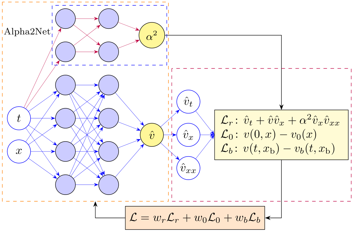
We employ a Physics-Informed Neural Network (PINN) to address both the inverse and forward problems for the Leray-Burgers (LB) equation, as depicted in Figure 1. The LB equation, given by
is solved in various initial and boundary condition scenarios, with the characteristic wavelength parameter , fixed () or adaptively optimized(). The PINN architecture, shown in Figure 1, consists of two primary components: a main neural network to approximate the solution and a subnetwork, Alpha2Net, to learn the parameter . The main network is a fully connected feed-forward neural network (multilayer perceptron, MLP) with eight hidden layers, each containing 20 neurons, and employs activation functions. It takes spatio-temporal coordinates and as inputs and outputs the predicted solution . To enforce the physics of the LB equation, automatic differentiation is used to compute the derivatives , , and , which are then used to evaluate the PDE residual.
The Alpha2Net subnetwork, highlighted in the upper part of Figure 1, is designed to adaptively learn the parameter as a function of time, i.e. . This subnetwork is a smaller MLP with three hidden layers, each containing 10 neurons, and also uses activation functions. It takes the time coordinate as its sole input and outputs , for use in the PDE residual. To ensure physical consistency, Alpha2Net constrains to lie within the range , slightly broader than the practical range identified in the inverse problem in Section 4. This slight extension allows computational flexibility while maintaining alignment with the physically meaningful bounds established earlier. The constraint is implemented by applying a sigmoid activation at the output layer of Alpha2Net, scaled to map the output to the desired range:
where is the raw output of the subnetwork. This ensures that remains within the specified bounds during training, preventing the network from converging to nonphysical values.
The output of the main network and Alpha2Net() are combined to compute the PDE residual, as shown in the right part of Figure 1. The loss function is designed to enforce the physics of the LB equation and consists of three key components:
-
•
Residual Loss (enforcing the PDE):
where is the number of collocation points sampled across the spatiotemporal domain.
-
•
Initial Condition Loss:
where is the number of points sampled along the initial condition at .
-
•
Boundary Condition Loss:
where is the number of points sampled along the boundary .
These terms are combined into a total loss
where the weights are either fixed (e.g., set to 1 for equal weighting) or tuned dynamically during training to balance the contributions of each loss term. The training points are adaptively sampled using Latin Hypercube Sampling, with a focus on regions exhibiting high PDE residuals or steep solution gradients, such as shock regions near discontinuities in the initial conditions.
The model is optimized using either the ADAM or Limited-Memory BFGS (L-BFGS) optimizer with a decaying learning rate schedule over unit epochs. During training, the parameters of both the main network (weights and biases) and Alpha2Net are updated simultaneously to minimize the total loss . Performance is assessed by computing the -error between the PINN predictions and the analytical solutions of the inviscid Burgers equation, obtained via the method of characteristics.
This architecture, as illustrated in Figure 1, effectively integrates the physical constraints of the LB equation into the neural network framework, allowing for both the approximation of the solution and the adaptive optimization of the regularization parameter . The use of Alpha2Net to learn within a constrained range ensures that the solutions remain physically meaningful, bridging the inverse and forward problems seamlessly.
4 Inverse Problem for the Estimation of Parameter
We set up the computational frame for the governing system (2.1) by
| (4.1) | |||
| (4.2) | |||
| (4.3) |
where is a bounded domain, is a boundary of , is an initial distribution, and is a boundary data. We intentionally introduced a new parameter and set . During the training process, the PINN will learn to determine the validity of the obtained for the inviscid Burgers equation () along with the relative errors. We use numerical or analytical solutions of the exact inviscid and viscous Burgers equations to generate training data sets with different initial and boundary conditions:
where denotes the output value at position and time with the final time . refers to the number of training data. Our goal is to estimate the effective range of such that the neural network satisfies the equation (4.1)-(4.3) and . The selected training models represent a range of initial conditions, from continuous initial data to discontinuous data, displaying shock and rarefaction waves.
4.1 PINN for Inverse Problem
Following the original work of Raissi et al. [15, 14], we use a Physics-Informed Neural Network (PINN) to determine physically meaningful -values closely approximating the entropy solutions to the inviscid Burgers equation. For the inverse problem, Alpha2net in Figure 1 is not used because we are looking for a fixed value of . The PINN enforces the physical constraint,
on the MLP surrogate , where denotes all parameters of the network (weights and biases ) and the physical parameters in (4.1), acting directly in the loss function
| (4.4) |
where is the loss function on the available measurement data set that consists in the mean-squared-error (MSE) between the MLP’s predictions and training data and is the additional residual term quantifying the discrepancy of the neural network surrogate with respect to the underlying differential operator in (4.1). Note that with in Figure 1. We define the data residual at in :
and the PDE residual at in :
where . Then, the data loss and residual loss functions in (4.4) can be written as
The goal is to find the network and physical parameters and that minimize the loss function (4.4):
over an admissible set and of training network parameters and , respectively.
In practice, given the set of scattered data , the MLP takes the coordinate as input and produces output vectors that have the same dimension as . The PDE residual forces the output vector to comply with the physics imposed by the LB equation. The PDE residual network takes its derivatives with respect to the input variables and by applying the chain rule to differentiate the compositions of functions using the automatic differentiation integrated into TensorFlow. The residual of the underlying differential equation is evaluated using these gradients. The data loss and the residual loss are trained using input from across the entire domain of interest.
4.2 Experiment 1: Inviscid with Riemann Initial Data
We consider the inviscid Burgers equation (2.3) with some standard Riemann initial data of the form
We used the conservative upwind difference scheme to generate training data. For each initial profile, we computed data points throughout the entire spatiotemporal domain. We modified the code in [14] and, for each case, performed ten computational simulations with 2000 training data randomly sampled for each computation. We adopted the Limited-Memory BFGS (L-BFGS) optimizer with a learning rate of 0.01 to minimize MSE (4.4). When the L-BFGS optimizer diverged, we preprocessed with the ADAM optimizer and finalized the optimization with the L-BFGS. We manually checked with random sets of hyperparameters by training the algorithm and selected the best set of parameters that fit our objective, 8 hidden layers and 20 units per layer, epochs. We trained the other models with the same parameters, which might not be the best but reasonable fit for them. One remark is that our problem is identifying the model parameter rather than inferencing solutions, and it is unnecessary to consider physical causality in our loss function (4.4) as pointed out in [19].
Upon training, the network is calibrated to predict the entire solution , as well as the unknown parameters and . Along with the relative -norm of the difference between the exact solution and the corresponding trial solution
we used the absolute error of ,
in determining the validity of each computational result.
The practical range of was determined by ensuring the relative error remained below while , aligning the LB solution with the inviscid Burgers entropy solution. The results show that the value depends on the initial data, with the effective range of being between 0.01 and 0.05 for continuous initial profiles and between 0.01 and 0.03 for discontinuous initial profiles.
When appropriate, we will also measure the averaged relative error in time,
4.2.1 Shock Waves
We consider two different initial profiles that develop shocks:
with the initial data,
| (4.5) | ||||
The exact entropy solutions corresponding to the initial data (I) and (II) in (4.5) are
| (4.6) | ||||
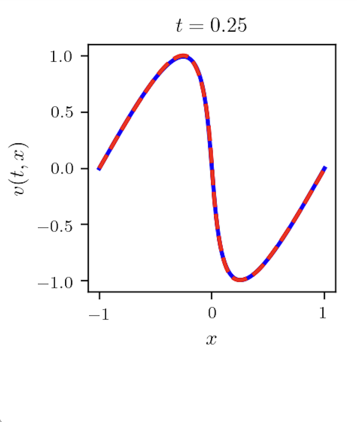
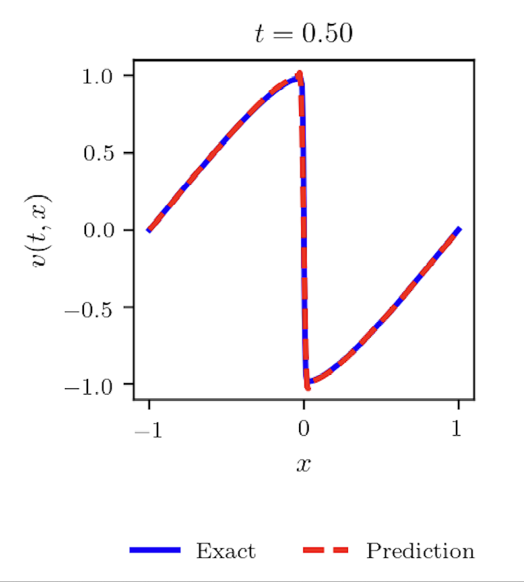
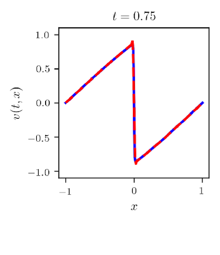
respectively. The initial profile (I) in (4.5) represents a ramp function with a slope of , which creates a wave that travels faster on the left-hand side of than on the right-hand side. The faster wave overtakes the slow wave, causing a discontinuity when , as we can see from the exact solution in (4.6). The second initial data (II) in (4.5) contains a discontinuity at . Its solution needs a shock fitting just from the beginning.
| No. | Initial Profile (I) | Initial Profile (II) | ||||
|---|---|---|---|---|---|---|
| 1 | 1.11e-3 | 3.4e-3 | 5.73e-3 | 6.76e-4 | 6.18e-2 | 7.16e-3 |
| 2 | 1.28e-3 | 6.6e-3 | 5.91e-3 | 4.46e-4 | 2.32e-2 | 3.70e-3 |
| 3 | 1.54e-3 | 1.24e-2 | 5.17e-3 | 4.85e-4 | 1.70e-2 | 5.31e-3 |
| 4 | 1.31e-3 | 1.33e-2 | 5.62e-3 | 5.69e-4 | 7.2e-3 | 5.92e-3 |
| 5 | 1.47e-3 | 6.2e-3 | 5.45e-3 | 6.53e-4 | 6.5e-3 | 7.77e-3 |
| 6 | 1.32e-3 | 6.1e-3 | 5.09e-3 | 8.41e-4 | 2.04e-2 | 1.04e-2 |
| 7 | 6.02e-4 | 1.03e-2 | 7.02e-3 | 8.76e-4 | 5.91e-2 | 1.09e-2 |
| 8 | 1.94e-3 | 6.7e-3 | 5.29e-3 | 8.77e-4 | 4.5e-3 | 1.23e-2 |
| 9 | 7.32e-4 | 5.6e-3 | 6.36e-3 | 9.17e-4 | 1.51e-2 | 1.76e-2 |
| 10 | 1.81e-4 | 1.24e-2 | 5.33e-3 | 7.64e-4 | 4.00e-4 | 9.83e-3 |
| Avg | 1.31e-3 | 8.30e-3 | 5.70e-3 | 7.11e-3 | 2.12e-2 | 9.09e-3 |
| 3.62e-2 | 2.67e-2 | |||||
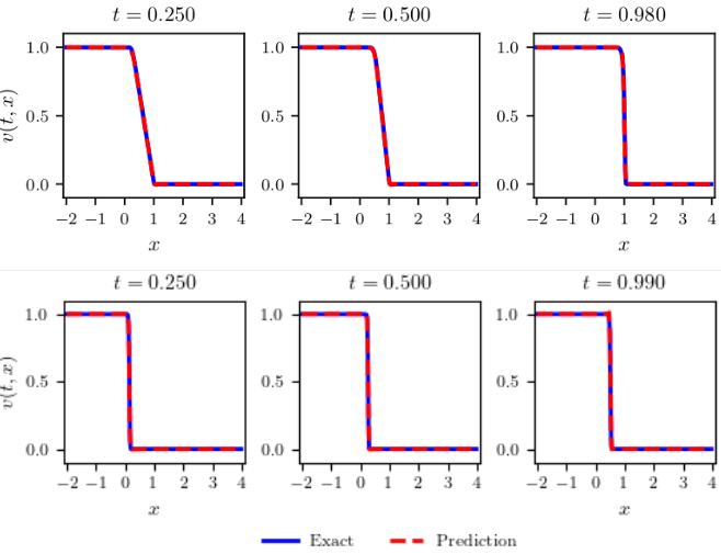
Based on the Rankine-Hugoniot condition, the discontinuity must travel at a speed , which we can observe in the analytical solution in (4.6). The solution also satisfies the entropy condition, which guarantees that it is the unique weak solution for the problem. Table 1 shows ten computational results.
In both cases, the average is within , indicating that the inferred PDE residual reflects the actual Leray-Burgers solutions within an acceptable range. The average value of with the initial profile (I) was with . Figure 2 shows a plot example. We can see that the Leray-Burgers solution captures well the shock wave and maintains the discontinuity at as evolves to . Computations with the initial profile (II) resulted in on average with . Figure 2 shows that the Leray-Burgers equation captures the shock wave as well as its speed per unit time. Increasing the training data () did not change the value of significantly.
4.2.2 Rarefaction Waves
We generate a training data set from the inviscid Burgers equation
with the initial data
| (4.7) | ||||
The rarefaction waves are continuous self-similar solutions, which are
corresponding to the initial data (III) and (IV) in (4.7), respectively.
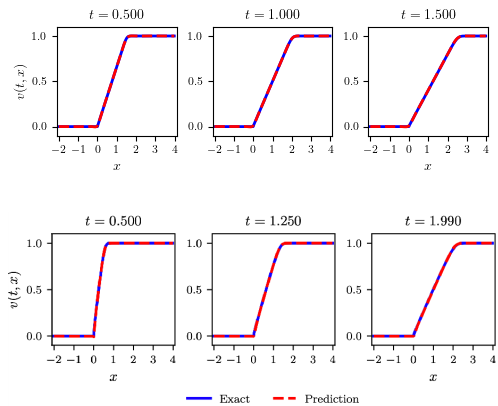
In both cases, is within , indicating that the inferred PDE residual reflects the Leray-Burgers equations within an acceptable range. The average value of are with for the continuous initial profile (III) and with for the discontinuous initial profile (IV). Figure 3 shows that the LB equation captures the rarefaction waves well.
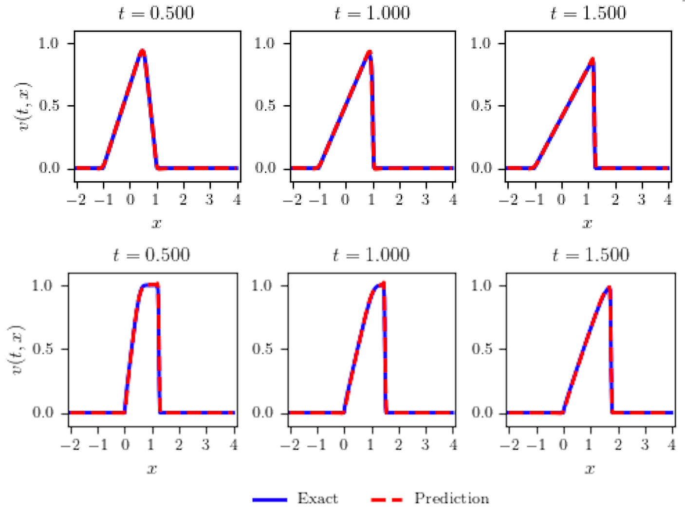
4.2.3 Shock and Rarefaction Waves
We combine the shock and rarefaction profiles:
In both cases, is within and the mean values of are with for the continuous initial profile (V) and with for the discontinuous initial profile (VI). Figure 4 shows that the LB equation captures both shock and rarefaction waves well.
4.3 Experiment 2: Viscid Cases
In this section, we consider the following viscous Burgers equation for a training data set:
| (4.8) |
with
The corresponding LB equation is
For the initial and boundary data (A), Rudy, et al., [16] proposed the data set that can correctly identify the viscous Burgers equation solely from time series data. It contains 101-time snapshots of a solution to the Burgers equation with a Gaussian initial condition propagating into a traveling wave. Each snapshot has 256 uniform spatial grids. For our experiment, we adopt the data set prepared by Raissi, et all, in [15, 14] based on [16], data points, generated from the exact solution to (4.8). For training, collocation points are randomly sampled and we use the L-BFGS optimizer with a learning rate of 0.8. The average of ten experiments is with . The computational simulation shows that the equation develops a shock properly (Figure 5). Note that .
For the initial and periodic boundary condition (B), we generate training data from the exact solution formula for the whole dynamics over time. With training data, the PINN diverges frequently. We experiment with the model with 4000 or more data points to determine an appropriate number of training data. error remains around for all cases, which does not provide a clear cut. So, we use the absolute error of to determine the appropriate number of training data. For each case of , we perform the computation 5 to 10 times (Table 2).
| 4000 | 6000 | 8000 | 10000 | 12000 | 14000 | |
|---|---|---|---|---|---|---|
| 0.0207 | 0.0113 | 0.01059 | 0.00965 | 0.00908 | 0.00848 | |
| 16000 | 18000 | 20000 | 25000 | 30000 | ||
| 0.0046 | 0.0059 | 0.00604 | 0.00671 | 0.00611 |
As increases, the results get better and need to do until it reaches the upper limit. Errors between 14000 and 18000 look better than other ranges. More than 18000 does not seem to improve the results. (12.5% of total data) is chosen. More than this does not seem to be better. More likely almost the same. The average of ten computations is with . Observe that .
Every part of the solution for (B) moves to the right at the same speed, which differs from (A) (Fig. 6). In (A), the left side of a peak moves faster than the right side, developing a steeper middle. It resulted in a higher value of with (B) than with (A).
In summary, we observe that with the profile (A) and with the profile (B). These results demonstrate that the LB equation can capture nonlinear interactions at significantly smaller length scales compared to the viscous Burgers equation. Notably, numerical schemes for the viscous Burgers equation become unstable at lower values, whereas the LB equation maintains stability and convergence under these conditions. This observation will be clearer when we compare the forward inferred solutions of two equations in Section 5 (Part C).
4.4 Experiment 3: The Filtered Vector
We write Equation (2.1) in the filtered vector , which is a quasilinear evolution equation that consists of the inviscid Burgers equation plus nonlinear terms [2, 3, 4]:
| (4.9) |
We compute the equation with the same conditions as in the previous corresponding experiments. The results show that the filtered equation (4.9) also tends to depend on the continuity of the initial profile as shown in Table 3.
| IC | Continuous | IC | Discontinuous |
|---|---|---|---|
| I | 0.0279 | II | 0.0004 |
| III | 0.0469 | IV | 0.0127 |
| V | 0.0469 | VI | 0.0277 |
When initial profiles contain discontinuities, the values are much smaller than those with continuous initial profiles. Compared to the unfiltered equation (2.1), the values for the filtered equation (4.9) are smaller, which may cause more oscillation in forward inference.
With the initial profile (II), the parameter for the filtered velocity is not close to 1 with on average. By increasing the number of epochs from 10000 to 50000 we get a better result. gets closer to 1 with , slightly better relative error and loss, which makes the solution better at later time. The oscillation near the discontinuity gets reduced. This verifies that needs very small values to approximate the inviscid Burgers solution.
Having established ’s practical range, we next explore its application in forward inference.
5 Data-Driven Solutions of the Leray-Burgers Equation
In this section, we solve the LB equation across multiple initial and boundary condition scenarios:
with
Training utilizes initial condition points, boundary condition points, and collocation points. These points are adaptively sampled using Latin Hypercube Sampling, with an emphasis on regions exhibiting high PDE residuals or steep solution gradients, particularly in shock regions near discontinuities identified in the initial condition. Our computational focuses are as follows:
-
1.
Convergence in . Whether the PINN solutions converge to those of the inviscid Burgers equation as .
-
2.
Forward inference with adaptive . Whether the PINN solutions capture the shock and rarefaction waves well and whether the trained values are within the physically valid range.
-
3.
Scaling effect of the parameter relative to the inviscid and viscous Burgers equation.
5.1 The Convergence of the Leray-Burgers Solutions as
Figure 8 demonstrates that the Leray-Burgers equation effectively captures the shock formation with the continuous initial profile (I) within the range of . As , the LB solution converges to the inviscid Burgers solution (the last graph in Figure 8).
With the discontinuous initial file (II), the Leray-Burgers equation still accurately captures the shock formation within the range of (Figure 9). However, the MLP-based PINN generates spurious oscillations near the discontinuity at the beginning. Although the network quickly recovers and fits the oscillations as time progresses, the oscillations worsen, and nonlinear instability arises as the scale becomes smaller than 0.01, which leads to the deviation of the network solution from the actual inviscid Burgers solution (the last graph in Figure 9).
5.2 Forward Inference with Adaptively Optimized
In this section, we employ the MLP-based Physics-Informed Neural Network (MLP-PINN) to effectively learn the nonlinear operator , wherein represents the primary variable and denotes a parameter. Coutinho, et all., [5], introduced the idea of adaptive artificial viscosity that can be learned during the training procedure and does not depend on the a priori choice of artificial viscosity coefficient. Instead of incorporating the parameter in place of the artificial viscosity as in [5], we set up a dedicated subnetwork, Alpha2Net depicted in Figure 1, to find the optimal value. The integration of the subnetwork into the main PINN architecture makes PINN train both and to achieve a robust fit with the LB equation. Two examples highlight the ability of the LB equation to capture shock and rarefaction waves as well as the corresponding optimal values of , which are presented in Figure 10.
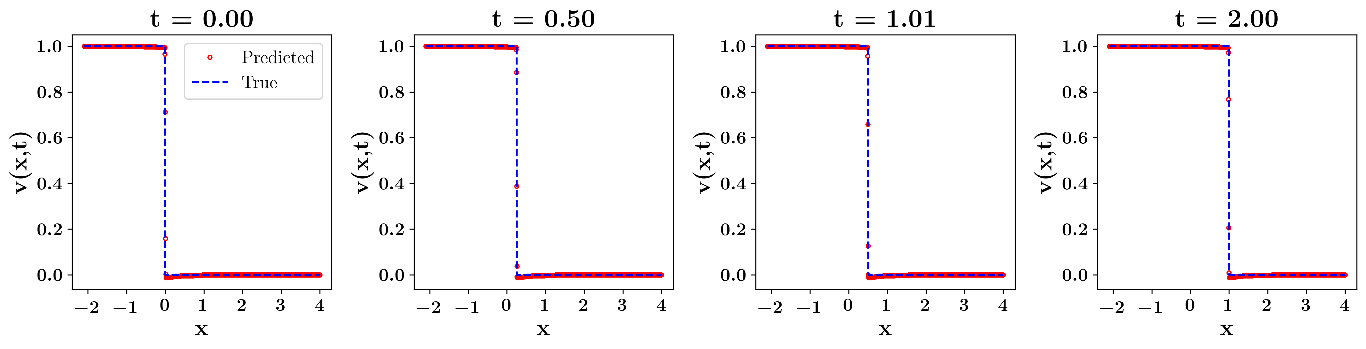
For the computations, we generated training data in the domain from the corresponding analytical solution for each case. With , , and epochs =20000. The first graph presents computational snapshots of the system’s evolution with the initial profile (II) over the time interval [0, 2]. The computational outputs are and the averaged relative -error in time is around with . Note that is the average of trained values of over time. The second graph illustrates snapshots of the evolution of a rarefaction wave with the initial profile (IV). The computational outputs are and the averaged relative error in time is around with the averaged in time.
5.3 The Effect of Scale in Relation to the Inviscid and Viscous Burgers Equations
When comparing the Leray-Burgers equation (2.1) with the viscous Burgers equation (4.8), the term in (2.1) serves as a nonlinear regularization mechanism, acting as a substitute for the linear diffusion term in the viscous Burgers equation. Unlike linear diffusion, the term in Equation (2.1) depends on both the first derivative and the second derivative , suggesting that its smoothing effect is more pronounced in regions with high gradients, modulated by the parameter . Thus, it is valuable to assess the performance of these two equations in relation to the inviscid Burgers equation.
Both equations are solved using PINNs with consistent training configurations: 20,000 epochs, fixed weights, and identical network architectures (8 hidden layers, 20 neurons per layer). The key metric for comparison is the error, which quantifies the difference between the predicted and exact solutions, with lower values indicating better accuracy. Computations provide errors for both equations across different values of , with set equal to in the viscous Burgers equation (4.8). The averaged errors over time are summarized in Table 4.
| LB Average | VB Average | ||
|---|---|---|---|
| 0.025 | 0.000625 | ||
| 0.030 | 0.0009 | ||
| 0.032 | 0.001024 | ||
| 0.033 | 0.001089 | ||
| 0.035 | 0.001225 |
For values ranging from 0.025 to 0.033 ( from 0.000625 to 0.001089), the LB equation consistently outperforms the viscous Burgers equation in the averaged error. The averaged error for LB equation remains relatively stable, ranging from to . In contrast, the Burgers equation exhibits higher errors, ranging from to . There is no clear monotonic trend, indicating variability in the neural network’s ability to approximate the solution.
These results indicate that for small values of , the viscous Burgers equation is prone to developing shocks due to its hyperbolic nature. PINNs may struggle to accurately capture these discontinuities. In contrast, the LB equation, through its nonlinear regularization effect (dependent on ), likely smooths these discontinuities, leading to improved accuracy.
The data also suggest a tipping point between (), where the performance of the two models being to shift. A more definitive transition appears to occur between and (), at which point the viscous Burgers equation begins to outperform the LB equation. This transition is illustrated in Figure 11.
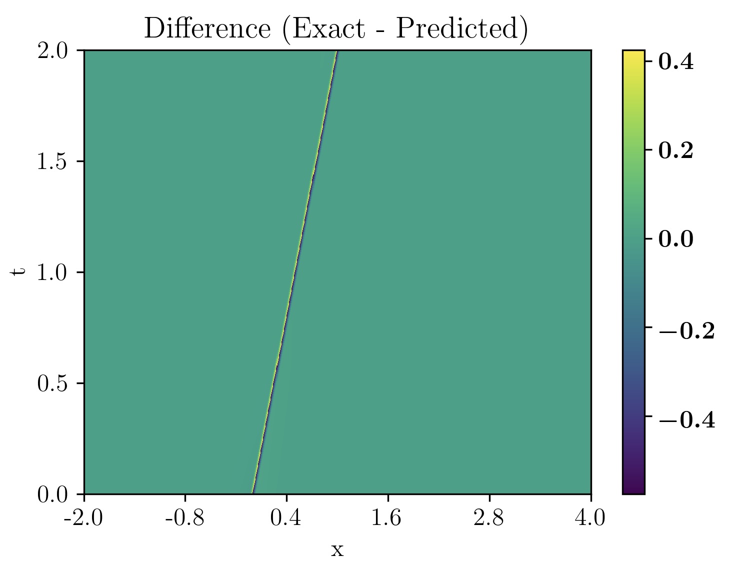
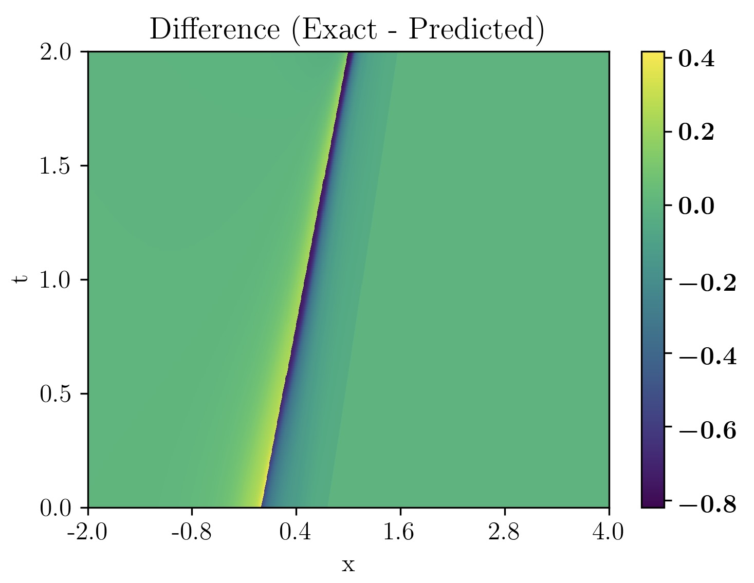
To further examine the differences in solution behavior, Figure 12 presents heatmaps of the difference between the solutions of the LB equation and the inviscid Burgers equation, as well as the difference between the viscous Burgers equation and the inviscid Burgers equation, for (). The LB equation exhibits a more gradual transition in error distribution, while the viscous Burgers equation shows sharper localized discrepancies along the shock region. This suggests that the nonlinear regularization in LB equation helps mitigate sharp discontinuities, leading to improved prediction accuracy.
In summary, the parameter (through ) controls the regularization strength. Smaller values of correspond to finer scales where regularization enhances accuracy, while larger values increase , potentially leading to over-smoothing compared to the standard viscous Burgers equation. In practice, the LB equation may be preferable for smaller length scales (low ), while the viscous Burgers equation may be more suitable for larger scales (higher ). The transition appears to occur near . These findings emphasize the interplay between physical regularization, viscosity, and the numerical approximation capabilities of PINNs.
6 Application to Traffic State Estimation
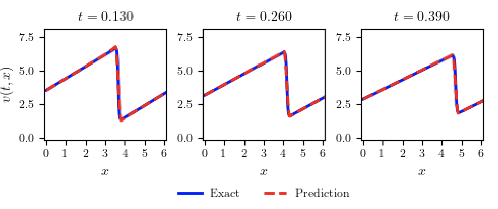
This section demonstrates the practical utility of forward inference with the LB equation, using the estimated range to model traffic dynamics efficiently. Huang, et all., [9] applied PINNs to tackle the challenge of data sparsity and sensor noise in traffic state estimation (TSE). The main goal of TSE is to obtain and provide a reliable description of traffic conditions in real time. In Case Study-I in [9], they prepared the test bed of a 5000-meter road segment for 300 seconds . The spatial resolution of the dataset is 5 meters and the temporal resolution is 1 second. The case study was designed to utilize the trajectory information data from Connected and Autonomous Vehicles (CAVs) as captured by Roadside Units (RSUs), which were deployed every 1000 meters on the road segment (6 RSUs on the 5000-meter road from ). The communication range of RSU was assumed to be 300 meters, meaning that vehicle information broadcast by CAVs at can be captured by the first RSU and the second RSU can log CAV data transmitted at , etc. More details on data acquisition and description can be found in [9, 10].
In this section, we switch to the differential notation to avoid confusion with constant parameter notations such as . Let denote the flow rate indicating the number of vehicles that pass a set location in a unit of time and the flow density representing the number of vehicles in a unit road of space. Then, the Lighthill-Whitham-Richards (LWR) traffic model [9] is, for ,
| (6.1) |
where and . Here is the cumulative flow that depicts the number of vehicles that have passed location by time . Huang, et all., [9] adopted the Greenshields fundamental diagram to set the relationship between traffic states - density , flow , and speed :
| (6.2) | ||||
where is the jam density (maximum density) and is the free-flow speed. Substituting the relationship (6.2) into (6.1) transforms the LWR model into the LWR-Greenshield model
| (6.3) |
We will just call it the LWR model. The equation (6.3) is a hyperbolic PDE and a second order diffusive term can be added as following, to make the PDE become parabolic and secure a strong solution:
| (6.4) |
We will call the equation (6.4) the LWR- model. The second-order diffusion term ensures that the solution of PDE is continuous and differentiable, avoiding breakdown and discontinuity in the solution. Following the same structural idea from (6.3) to (6.4) we add a regularization term to (6.3) instead of the diffusion term in (6.4):
| (6.5) |
We will call Equation (6.5) the LWR- model. We set up the same PINN architecture for computational comparisons of three models, LWR, LWR-, and LWR-, with . Figure 13 visualizes the computational results.
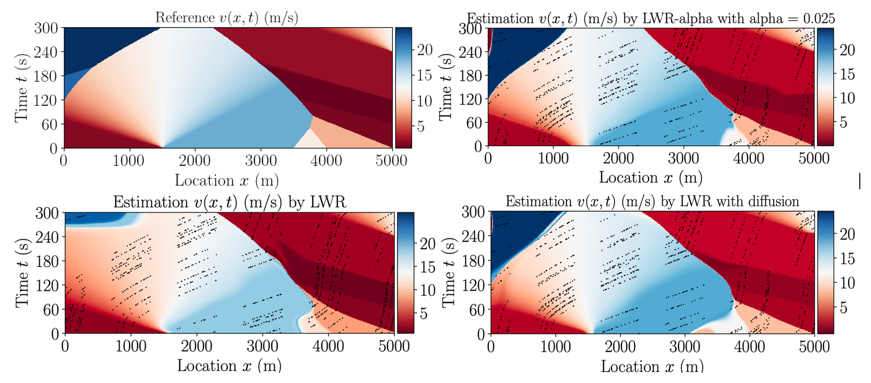
Our empirical calculations demonstrate that both the LWR- and LWR- models provide reasonable approximations of the reference speed (), as illustrated in Figure 13. Both models exhibit comparable accuracy to the standard LWR model, validating their potential for traffic state estimation applications.
The experiments highlight the critical role of nonlinear characteristics in traffic data for accurate state estimation. The LWR- model emerges as the more practical choice due to its superior ability to capture the inherent nonlinear behavior of traffic flow. While the LWR- model offers a reasonable approximation, its limited computational performance at lower scales (below 0.025) restricts its utility in real-time applications.
In our traffic state estimation (TSE) application, we employed the LWR- model with . This parameter value directly addresses our primary objectives of determining the practical range of in the Leray-Burgers equation and evaluating the effectiveness of Physics-Informed Neural Networks (PINNs) in solving the forward inference problem. The chosen value of aligns closely with the estimated range of the inverse problem: specifically 0.01 to 0.05 for continuous initial profiles and 0.01 to 0.03 for discontinuous profiles.
The successful application of the LWR- model in accurately capturing the dynamics of traffic flow validates the physical relevance and practicality of our estimated range. Moreover, the robust performance of PINNs in precisely estimating traffic states using this model demonstrates their effectiveness in solving the forward inference problem for the Leray-Burgers equation. Consequently, our TSE results substantiate both the accuracy of our estimation and the capabilities of PINNs, thereby reinforcing the core findings of our study and affirming their potential in real-world applications.
7 Discussion
The relationship between the inverse and forward problems is a cornerstone of our approach to solving the Leray-Burgers (LB) equation with Physics-Informed Neural Networks (PINNs). In the inverse problem, we determine the practical range of the characteristic wavelength parameter that ensures that the LB equation closely approximates the inviscid Burgers solution. This range, derived from the training of PINNs on inviscid Burgers data, reflects the values of that maintain the physical fidelity of LB solutions under a variety of initial conditions.
This estimation is not an isolated step, but directly informs the forward inference process. When training PINNs to solve the LB equation, we do not prescribe a fixed . Instead, is treated as a trainable parameter, optimized concurrently with the standard PINN parameters (weights and biases) through a subnetwork called Alpha2Net. To ensure that the optimized remains physically meaningful, Alpha2Net enforces a constraint: must be within the range established by the inverse problem. This restriction serves a dual purpose: it prevents the network from converging to nonphysical or suboptimal values of , and it leverages the prior knowledge gained from the inverse problem to improve the accuracy and stability of the forward solutions. For example, if the inverse problem indicates that should range between 0.01 and 0.05 for certain profiles, Alpha2Net ensures that the learned during forward inference adheres to these bounds. This linkage guarantees that the solutions to the LB equation not only capture complex phenomena like shocks and rarefactions but also remain consistent with the physical constraints established earlier. Thus, the inverse problem provides an essential scaffold that supports and refines forward inference, creating a unified framework for parameter estimation and PDE solution.
8 Conclusion
Computational experiments show that the -values depend on the initial data. Specifically, the practical range of spans from 0.01 to 0.05 for continuous initial profiles and narrows to 0.01 to 0.03 for discontinuous profiles. We also note that the Leray-Burgers equation in terms of the filtered vector does not produce reliable estimates of . When approximating the filtered solution with commendable precision, MLP-PINN necessitates a more extensive dataset, and the range of values for appears confined, between 0.0001 and 0.005. Nonetheless, the MLP-PINN’s attempts with encounter challenges in converging to the true Burgers solutions. Thus, it is evident that the equation formulated in the unfiltered vector field offers a better approximation to the exact Burgers equation.
In practical terms, treating as an unknown variable becomes a prudent strategy. By endowment with learnable attributes along with network parameters, MLP-PINNs can be structured to reveal within a valid range during the training process, potentially improving accuracy. Nevertheless, the MLP-PINN does generate spurious oscillations near discontinuities inherent in shock-inducing initial profiles. This phenomenon thwarts the PINN solution from aligning with an exact inviscid Burgers solution as .
This study also demonstrates the effectiveness of the LWR- model as a viable alternative for traffic state estimation. Surpassing the diffusion-based LWR- model in terms of computational efficiency, the LWR- model aligns with the nonlinear nature of traffic data.
Statements and Declarations
Competing Interests: On behalf of all authors, the corresponding author states that there is no conflict of interest.
Data Availability: The code and data we used to train and evaluate our models are available at
https://github.com/bkimo/PINN-LB.
The data for traffic state estimations generated by Huang, et al. [9, 10] is available at
Acknowledgment
The second author was supported by the Research Grant of Kwangwoon University in 2022 and by the National Research Foundation of Korea(NRF) grant funded by the Korea government(MSIT) (No. 2021R1F1A1058696). The third author gratefully acknowledge the Advanced Technology and Artificial Intelligence Center at American University of Ras Al Khaimah for providing high-performance GPU computing resources to support this research.
References
- [1] Raul K.C. Araújo1, Enrique Fernández-Cara, and Diego A. Souza. On the uniform controllability for a family of non-viscous and viscous burgers- systems. ESAIM: Control, Optimisation and Calculus of Variations, 27(78), 2021.
- [2] H. S. Bhat and R. C. Fetecau. A hamiltonian regularization of the burgers equation. Journal of Nonlinear Science, 16:615–638, 2006.
- [3] H. S. Bhat and R. C. Fetecau. Stability of fronts for a regularization of the burgers equation. Quarterly of Applied Mathematics, 66:473–496, 2008.
- [4] H. S. Bhat and R. C. Fetecau. The Riemann problem for the leray-burgers equation. Journal of Differential Equations, 246:3597–3979, 2009.
- [5] Emilio Jose Rocha Coutinho, Marcelo Dall’Aqua, Levi McClenny, Ming Zhong, Ulisses Braga-Neto, and Eduardo Gildin. Physics-informed neural networks with adaptive localized artificial viscosity. Journal of Computational Physics, 489(112265), 2023.
- [6] Georg A Gottwald. Dispersive regularizations and numerical discretizations for the inviscid burgers equation. Journal of Physics A: Mathematical and Theoretical, 40(49), 2007.
- [7] Billel Guelmame, Stéphane Junca, Didier Clamond, and Robert Pego. Global weak solutions of a hamiltonian regularised burgers equation. Journal of Dynamics and Differential Equations, 2022.
- [8] Darryl D. Holm, Chris Jeffery, Susan Kurien, Daniel Livescu, Mark A. Taylor, and Beth A. Wingate. The lans- model for computing turbulence: Origins, results, and open problems. Los Alamos Science, 19, 2005.
- [9] Archie J. Huang and Shaurya Agarwal. Physics-informed deep learning for traffic state estimation: Illustrations with LWR and CTM models. IEEE Open Journal of Intelligent Transportation Systems, 3, 2022.
- [10] Archie J. Huang and Shaurya Agarwal. On the limitations of physics-informed deep learning: Illustrations using first-order hyperbolic conservation law-based traffic flow model. IEEE Open Journal of Intelligent Transportation Systems, 4, 2023.
- [11] Traian Iliescu, Honghu Liu, and Xuping Xie. Regularized reduced order models for a stochastic burgers equation. International Journal of Numerical Analysis and Modeling, 15(4-5):594–607, 2018.
- [12] J. Leray. Essai sur le mouvement d’un fluide visqueux emplissant l’space. Acta Math., 63:193–248, 1934.
- [13] Yekaterina S. Pavlova. Convergence of the leray -regularization scheme for discontinuous entropy solutions of the inviscid burgers equation. The UCI Undergraduate Research Journal, pages 27–42, 2006.
- [14] M. Raissi, P. Perdikaris, and G.E. Karniadakis. Physics informed deep learning (part ii): Data-driven discovery of nonlinear partial differential equations. 2017. Preprint at https://arxiv.org/abs/1711.10566.
- [15] M. Raissi, P. Perdikaris, and G.E. Karniadakis. Physics-informed neural networks: A deep learning framework for solving forward and inverse problems involving nonlinear partial differential equations. Journal of Computational Physics, pages 686–707, 2019.
- [16] S.H. Rudy, S.L. Brunton, J.L. Proctor, and J.N. Kutz. Data-driven discovery of partial differential equations. Science Advances, 3, 2017.
- [17] Feriedoun Sabetghadam and Alireza Jafarpour. regularization of the pod-galerkin dynamical systems of the kuramoto–sivashinsky equation. Applied Mathematics and Computation, 218:6012–6025, 2012.
- [18] John Villavert and Kamran Mohseni. Physics-informed neural networks: A deep learning framework for solving forward and inverse problems involving nonlinear partial differential equations. Journal of Computational Physics, 378:686–707, 2019.
- [19] Sifan Wang, Parsi Perdikaris, and Shyam Sankaran. Respecting causality for training physics-informed neural networks. Computer Methods in Applied Mechanics and Engineering, 421(116813), 2024.
- [20] Ting Zhang and Chun Shen. Regularization of the shock wave solution to the riemann problem for the relativistic burgers equation. Abstract and Applied Analysis, 2014, 2014.
- [21] Hongwu Zhao and Kamran Mohseni. A dynamic model for the lagrangian-averaged navier-stokes- equations. Physics of Fluids, 17(075106), 2005.