Parameter Estimation from ICC curves
Abstract.
Incidence vs Cumulative Cases (ICC) curves are introduced and shown to provide a simple framework for parameter identification in the case of the most elementary epidemiological model, consisting of susceptible, infected, and removed compartments. This novel methodology is used to estimate the basic reproduction ratio of recent outbreaks, including the ongoing COVID-19 epidemic.
Key words and phrases:
Outbreak; Parameter Identification; Compartmental Models1. Overview
This article introduces the concept of ICC (Incidence vs Cumulative Cases) curves, which are nonlinear transformations of the traditional ‘EPI curves’ (plots of disease incidence versus time) commonly used by epidemiologists. The main message of the present work is that describing an outbreak in terms of its associated ICC curve is not only natural from a dynamical point of view, but also advantageous for parameter identification and forecasting purposes. Specifically, we provide a method for the practical identification of epidemiological parameters of the SIR (Susceptible - Infected - Removed) compartmental model, directly from its associated ICC curve. Because the result is robust to under-reporting, this approach gives a simple way to estimate the basic reproduction ratio of a disease from reported incidence data. The present analysis also provides a theoretical justification for the forecasting methodology put forward in [1], which was shown to lead to useful estimates of the characteristics (expected duration, final number of cases, and peak intensity) of ongoing outbreaks.
We develop the concept of ICC curves in the context of the classical SIR model [2, 3], which is the simplest compartmental model that captures the basic phenomenon of disease transmission: before recovering (or being removed through disease-induced death), infected individuals transmit the disease to susceptible individuals, who in turn become infected. The process repeats itself until the epidemic has followed its course and no additional infections occur. Since many outbreaks have a time scale that is much shorter than the scale at which the total population changes, a common simplification is to assume that is constant. It is then natural to define the time-dependent quantities and as the expected sizes of the susceptible (), infected (), and recovered () compartments relative to so that The resulting SIR model is then given by
where is the contact rate of the disease and is its recovery rate. Scaling time by turns the above equations into a one-parameter () model, where is the basic reproduction ratio [4, 5, 6] of the modeled epidemic. The disease spreads if and dies out when It is also clear from the right-hand side of the second SIR equation that for the proportion of infected individuals grows as a function of time as long as
In a compartmental model, an outbreak is a trajectory that starts in the vicinity of the disease-free equilibrium and ends at the endemic equilibrium, when the number of infected individuals approaches zero. We define an ICC curve, where ICC stands for Incidence vs. Cumulative Cases, as a representation of the dynamics associated with an outbreak, in the plane of coordinates (cumulative cases) and (incidence). The following theorem, established in Section 2, gives an exact formulation of the ICC curves of the SIR model.
Theorem 1.
For a total susceptible population of size and each initial condition , the ICC curve of the SIR model is given by
| (1) |
where and the final number of cases, is the positive solution of the transcendental equation
| (2) |
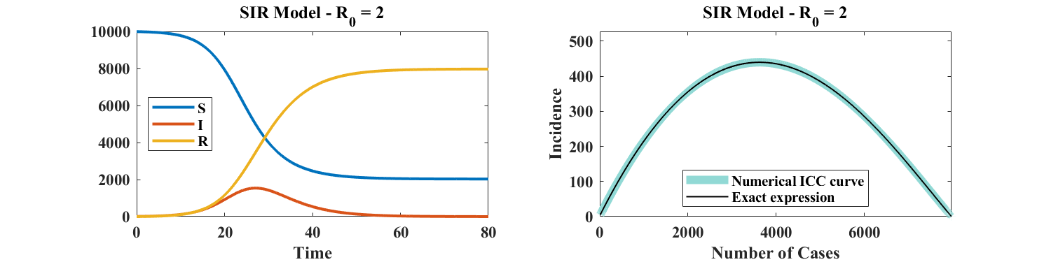
Details of the derivation of this theorem are given in Section 2.1. Its significance is illustrated in Figure 1, which shows a numerical simulation of the SIR model and a plot of the corresponding ICC curve for . Instead of considering the time dependence of , , and as shown in the left panel of Figure 1, the course of the outbreak is captured by a single curve: a plot of incidence versus cumulative cases. As explained in Section 2.1, knowledge of the ICC curve is sufficient to reconstruct the temporal behavior of , , and . In other words, the ICC curve contains the entire information associated with any outbreak described by the SIR model.
An important motivation for studying ICC curves is that they can easily be fitted to case data. Specifically, we show in Section 3.1 that, for fixed , there exists a single set of parameters that minimizes the root mean square error between (noisy) simulated outbreak data and the ICC curve given by Equation (1). Additionally, a numerical investigation indicates that such an estimation is robust to noise. As a consequence, the present approach provides a method to estimate the parameters of the SIR model, thereby making this model practically identifiable.
The rest of this manuscript is organized as follows. Section 2 presents the derivation of Equations (1) and 2, and discusses the robustness of ICC curves to systemic under- (or over-) reporting. Section 3 explains how model parameters may be retrieved from ICC curves and assesses the robustness of the proposed procedure to reporting noise. Section 4 briefly discusses parameter estimation as an outbreak unfolds. Section 5 shows a few examples of application to real data, for outbreaks of gastroenteritis and COVID-19. Future extensions and applications of the methodology proposed in this article are reviewed in Section 6.
2. ICC curves of the SIR Model
2.1. Proof of Theorem 1.1
Epidemiologists use the epidemiological (EPI) curve, a plot of incidence as a function of time, to visualize the course of an epidemic. In the SIR model, incidence is defined as
where is the cumulative number of cases at time Note that includes those who have recovered (and thus were a case at some point in time), as well as those who are currently infected. To derive Equation (1), write which can be integrated to give where is a constant that depends on initial conditions. Typically, (see e.g. [7]) since for an outbreak in a naive population we normally have and thus However here we do not make this assumption and keep the parameter in the following discussion. With and we obtain
and consequently
Moving back to dimensional variables gives the expression in Equation (1), i.e. .
An approximate expression of the SIR ICC curve, assuming and sufficiently small was given in [1]. Since on , for a given initial condition , the part of the ICC curve traced out as the outbreak unfolds will be such that . However, the ICC curve is well defined for in the range , which is the definition we adopt here. Even though the time variable does not appear in the ICC curve, the value of is not arbitrary: is the value of when , where represents the removed compartment.
ICC curves are particularly useful for forecasting the course of an outbreak because they contain information on quantities that are of interest to public health practitioners, namely the final number of cases () and peak incidence (). The latter is simply the maximum of ; the former may be found as follows. Since is the cumulative number of cases, it is a monotonic function of time and its derivative, must remain non-negative. For small,
where By continuity, will remain non-negative on the interval where is the unique positive solution of Equation (2). By writing Equation (2) as where the right-hand-side is the sum of two non-negative monotonic functions of , one increasing and the other decreasing, and since one can see that such a solution exists and is unique. Asymptotically, when the disease has followed its course and all infections have occurred, and Then, and the conservation law becomes In other words, defined in Equation (2) is simply the final (asymptotic) number of cases associated with the outbreak. This concludes the proof of Theorem 1.
To see that the entire dynamics of an outbreak in the SIR model is captured by the associated ICC curve, note that knowledge of leads to knowledge of
In other words, the time course of , , and may be obtained from the solution of the differential equation prescribed by the ICC curve, with appropriate initial conditions (which in turn define the value of ).
2.2. Robustness to under- or over-reporting
The quantity appearing in Equation (1) refers to the total population taken into account in the model, which is conserved by the dynamics. In case of over- or under-reporting, the observed incidence expectation is a fraction of the actual incidence , so that where we assume that is constant or varying slowly enough for its derivative to be negligible. The ICC curve estimated from case report data will then be a graph of as a function of We thus have
where . Therefore, the ICC curve in the presence of over-reporting () or under-reporting () has the same functional form, with the same parameter values, as the true ICC curve, provided , , and are rescaled by the factor . For the same reason, is also independent of the value of .
While systematic under- or over-reportding does not affect the ICC curve provided the size of each compartment is appropriately rescaled, the reproduction ratio depends on through the ratio , as can be seen from Equation (2), in which setting leads to
| (3) |
Finally, rescaling time amounts to rescaling and , and consequently the ICC curve.
3. Parameter identification
Structural identifiability (see e.g. [8] for a review) relates to the ability of uniquely identifying model parameters from knowledge of the model output. In this context, is assumed to be known since it represents the population of the system to which the model is applied. Given one can calculate From Equation (1), it is clear that knowledge of and uniquely determines and Indeed, if two sets of parameters, and , led to the same output (and thus to the same values of its derivative ), we would have
for all values of , which leads to , , and Therefore, all of the parameters of the SIR model, including initial conditions, are structurally identifiable from knowledge of the cumulative number of cases, and , the size of the susceptible population. Similar results were obtained in [9, 10, 11]. If is unknown, setting
for all values of , additionally leads to , making the size of the population a structurally identifiable parameter as well.
Whereas structural identifiability depends on the nature of the model itself, practical identifiability relates to parameter identifiability in the presence of measurement noise, as well as (hopefully small) deviations between model and reality (see e.g. [8]). This question may be addressed numerically by simulating an exact solution of the model, adding noise to its output, and estimating the model parameters that best fit the perturbed output. Two recent articles [11, 12] discuss the practical identifiability of a variety of compartmental models and reach different conclusions regarding parameter identification of the SEIR model from cumulative data. In [11], the cumulative data is multiplied by where is normally distributed with zero mean, whereas in [12], Poisson-distributed noise of mean equal to the current incidence value [13] is used as a substitute for the incidence data. Whether or not parameters are identifiable in practice therefore depends on the type of observational noise that affects surveillance reports and thus the EPI curve.
Adding independently-distributed noise to the incidence rather than the cumulative data is more realistic since errors on are considered to accumulate and not be independent [14]. On the one hand, assuming Poisson-type of uncertainty is natural for data that represent counts, but the effect of replacing incidence data by a Poisson random variable of same mean will lead to significant relative deviations only if is small (a few hundreds). For larger values of and thus of the relative change scales like Indeed,
With Stirling’s formula, we obtain
If it is believed that the diminishing relative influence of the Poisson-distributed noise for large values of is not realistic for a specific epidemic, then multiplying by where is normally distributed with mean zero, circumvents this issue. We consider both types of noise below.
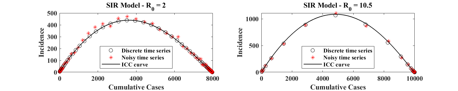
To test practical identifiability, we simulate the SIR model and generate a discrete time series for the cumulative number of cases of the simulated outbreak. This time series is used as a reference and represents the unperturbed (or true) data. We then add noise to the associated discrete incidence data (defined as the difference of cumulative values between consecutive time points), following the procedure described in [13], with the additional realistic constraint that the final number of cases is the same for all noisy realizations of the same outbreak. Two examples of simulated outbreaks generated in this fashion are shown in Figure 2 for different values of (associated with different orders of magnitude of the incidence ) and different discretization time steps . For , we use . For , we use As shown in Figure 2, this latter choice leads to a discretized ICC curve with very few points in regions of large incidence, and simulates a situation where incidence data is of poorer frequency. Each time series, consisting of noisy incidence data, is used to calculate an associated time series for the corresponding cumulative data. The resulting set of points is plotted in the (, ) plane, and defines an empirical ICC curve. In both panels of Figure 2, and are estimated from discrete incidence data as described in Equation (5) below.
3.1. Fitting ICC curves to data
Given a simulated time series for the number of cases of an outbreak in a population of size , we find the parameters of the ICC curve that best fits the data by least square minimization. This approach is different from parameter identification methods that have been proposed in the literature until now. Indeed, traditional methods aim to find the best combination of model parameters consistent with observed time series; they therefore require numerical integration of the compartmental model whose parameters need to be identified, in order to estimate and then minimize an associated cost function (see for instance [13, 11, 12]). Instead, the approach we put forward here consists in finding model parameters by directly fitting the relevant ICC curve to the data. We claim that this is a more robust approach because the functional that needs to be minimized has a unique extremizer in parameter space, which can be calculated exactly from the data points.
Given a time series of discrete incidences or of discrete cumulative cases recorded every units of time, we introduce a cost function that measures how much the data points depart from the ICC curve of the SIR model parametrized by and This function, , is defined by
| (4) |
where
and
| (5) |
A Maple [15] calculation shows that the cost function has a unique critical point, whose expression is given in Appendix A. For outbreaks that start in a naive population, the formulas are hugely simplified by setting . The resulting cost functional then has a unique minimum, whose value may easily be calculated. With the following notation,
we have (after setting ),
Setting the right-hand sides to zero and solving the resulting linear system for and leads to the following expression for the unique global minimizer of when :
where
In what follows, we use the expressions given in Appendix A, which can easily be coded up. We checked that for time series generated from an SIR model with , the simplified expressions above provide good estimates of the actual values of and that were used to generate the reference outbreak. Importantly, we now have a means of associating a single set of values for the parameters , , and to each outbreak time series.
3.2. Parameter identification in the presence of noise
We now use the expressions found in Section 3.1 to assess the robustness of the proposed parameter identification method to noise. As discussed above, the SIR model will be declared practically identifiable provided good estimates of the parameters may be obtained from noisy data. We therefore simulate 100,000 noisy time series from a ‘reference’ numerical integration of the SIR model, use the formulas of Appendix A to calculate , , and for each time series, and plot histograms of the estimated values of and . We consider the two types of noise discussed above, both affecting the reported discrete incidence In Case A, we assume that at each time point the reported value of has a Poisson distribution of mean In Case B, it is assumed that the reported value of at each time point is of the form where is the discrete incidence of the reference outbreak, is the noise amplitude, and is standard normal.
3.2.1. Case A: Poisson-distributed incidence
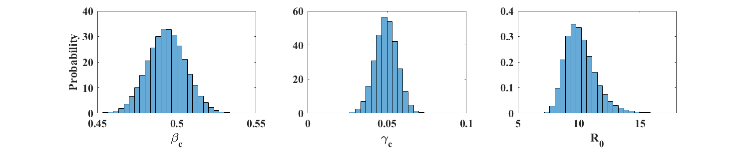
Figure 3 shows the distributions (in the form of properly scaled histograms) of and obtained from 100,000 noisy realization from a reference simulation of an SIR model with parameters and (). Figure 4 shows similar plots for and , so that . In each case, the size of the total population is individuals. The corresponding sample means and standard deviations are displayed in Table 1. These results indicate that the respective means of and provide very good estimates of the parameters and . Accuracy is not as good for the larger value of , whose distribution shows a fairly long tail. This is to be expected because the actual value of in this case is close to zero. Moreover, the number of data points away from the end points of the outbreak is much smaller for than for (see Figure 2), leading to a potential loss of information.
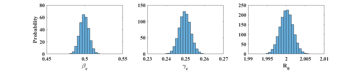
| 0.4994 | 0.0060 | 0.4936 | 0.0120 | |
| 0.2497 | 0.0030 | 0.0495 | 0.0070 | |
| 2.0001 | 0.0017 | 10.15 | 1.29 | |
3.2.2. Case B: Normally-distributed noise
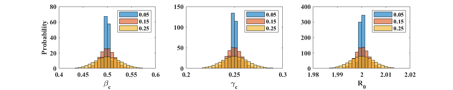
At each time point, we now multiply the reference incidence by , where is standard normal and the amplitude takes on one of 3 values: 0.05, 0.15, or 0.25. This type of noise is less realistic for incidence reports, whose variability is expected to be well described by a Poisson distribution, as in Case A above. We however perform the present tests to illustrate the robustness of the parameter estimation method introduced in this article.
| 0.4994 | 0.0048 | 0.5001 | 0.0152 | 0.5013 | 0.0267 | |
| 0.2497 | 0.0024 | 0.2500 | 0.0076 | 0.2506 | 0.0135 | |
| 2.0001 | 0.0009 | 2.0002 | 0.0028 | 2.0002 | 0.0050 | |
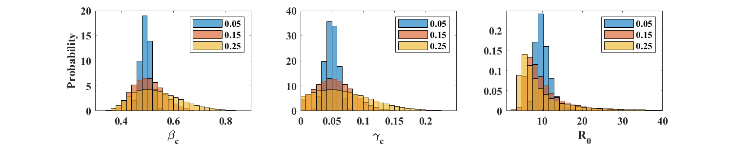
| 0.4939 | 0.0201 | 0.5053 | 0.0577 | 0.5396 | 0.0938 | |
| 0.04961 | 0.0104 | 0.0550 | 0.0293 | 0.0717 | 0.0465 | |
| 10.3682 | 2.14 | 27.0950 | 769.77 | 29.9396 | 863.86 | |
For , the parameter estimation procedure is robust at all values of considered. Means and standard deviations of , , and are displayed in Table 2. The corresponding distributions are shown in the top row of Figure 5. As expected, estimates of and are not as accurate for simulations with , but return mean values for and that are close to the exact values. The distributions of however shows very long tails (see bottom row of Figure 5), due to values of close to zero. In such a case, estimating as the ratio however gives acceptable values, equal to 9.96, 9.19, and 7.53, for equal to 0.05, 0.15, and 0.25 respectively.
In summary, the above numerical simulations indicate that the ICC-based parameter estimation method presented here provides good results in the presence of reporting noise. Not surprisingly, the quality of the estimates depends on the rate at which incidence is sampled and, in the case of normally distributed noise, on the amplitude of the noise.
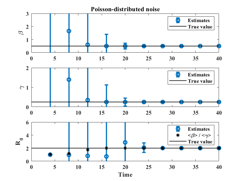
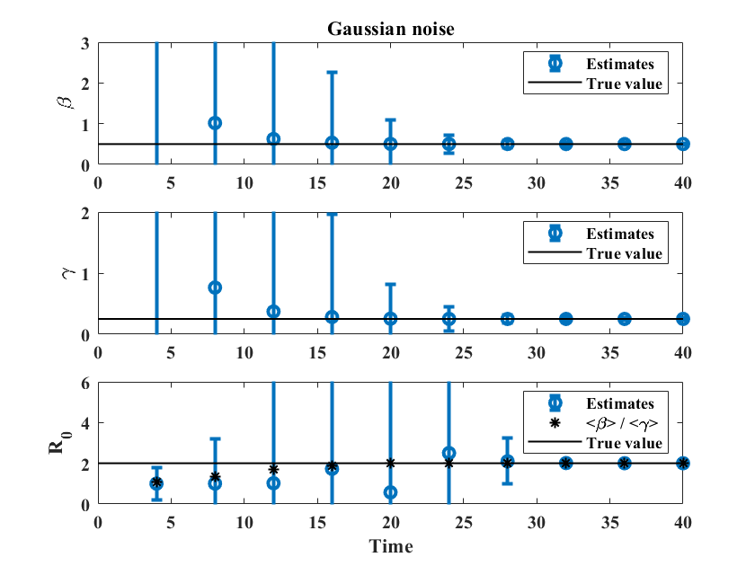
4. Parameter identification as the outbreak unfolds
In principle, the formulas for and given in Appendix A may be used with any number of points , as long as the data points represent the entire ICC curve. Is is natural to ask how the method performs when applied to a developing outbreak. To test this, we simulate 50,000 possible outbreaks using the same reference simulations as before, and with the two different types of noise introduced above to represent reporting error. We then follow the evolution of the distributions of the estimated parameters as time increases. For , the outbreak has run its course after 60 units of time, and we include up to data points, with consecutive values separated by 1 unit of time (which could correspond to a day or a week depending on the disease). For , we pick , with data points separated by 2 units of time. Figure 6 shows estimated values of , , and for the two types of reporting noise. In both cases, estimates of and are close to their actual values near , which is before the peak of the outbreak (see left panel of Figure 1). The value of converges more slowly (circles in the bottom row of Figure 6) but the ratio of the estimated values of and (stars) is close to the actual value of near , fairly early in the outbreak.
Similar results for , together with plots showing the evolution of the distributions of , , and , are provided as supplementary material. Parameter estimates for and are close to their true values near , which is near the peak of the outbreak, with the ratio giving a reasonable estimate of starting at , even in the presence of large uncertainty.
5. Application to outbreak data
So far, we have assumed the size of the susceptible population, , to be known. In practice, the value of that should be used to fit the ICC curve to outbreak data is often unknown since it may reflect under-reporting (as discussed in Section 2.2) or spatial effects (existence of localized clusters to which the spread is restricted) associated with the outbreak. Moreover, it could be argued that the SIR model is too simplistic to represent real-life outbreaks. The examples of [1] and those discussed below however show there is merit to the present approach.
In what follows, we fit ICC curves to surveillance reports by picking a range of values of for which the root mean square error (RMSE) between the ICC curve and the data is within 2% of the minimum RMSE value. The data points used in the evaluation of the RMSE are found from the reported cumulative data after smoothing and interpolation. This latter procedure estimates missing incidence values and removes negative incidence reports, if any. The resulting time series is expected to be a better approximation of the ‘true’ (i.e. as close as possible to the output of a compartmental model) evolution of the cumulative data, and is used for the parameter estimation procedure discussed in this article. Our first example is a gastroenteritis outbreak in a nursing home in Mallorca, Spain, and is therefore spatially localized. The other examples are estimations of the basic reproduction ratio for COVID-19 outbreaks in Hubei Province (China), the Republic of Korea, and France, based on data available until 4/15/2020.
5.1. Gastroenteritis outbreak in Mallorca, Spain
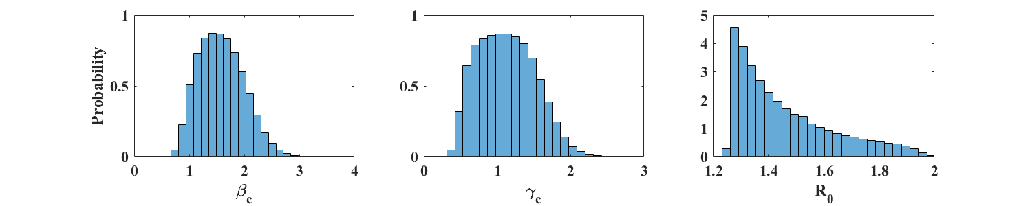
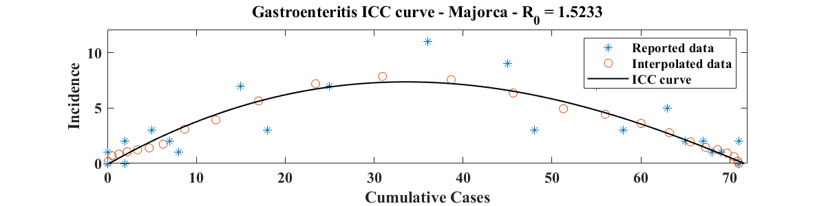
We use the same data set as in [1], estimated from the epidemiological curve provided in [16]. We fit the ICC curve to the interpolated data (i.e. find , , and ) for a range of values of , identify the value of that best fits the data (i.e. for which the RMSE is minimum), and select a range of values of near that give a RMSE within 2% of its minimum. Then, for each value of in the selected range, we apply the parameter estimation procedure of Section 3, with 10,000 oubreak realizations, obtained from adding Poisson-distributed noise to the smoothed and interpolated data. Figure 7 shows the resulting parameter distributions (top panel; ) and a plot of the ICC curve for the optimal parameter values (bottom panel; , , and ). The value of for the ICC curve displayed is and corresponds to an attack rate of 59.8%. This is near the upper boundary of the 95% confidence interval (38.5 % - 61.3 %) for the overall attack rate, but well within the 95% confidence interval of the attack rate among nursing home residents (42.1 % - 72.2 %) reported in [16].
5.2. COVID-19
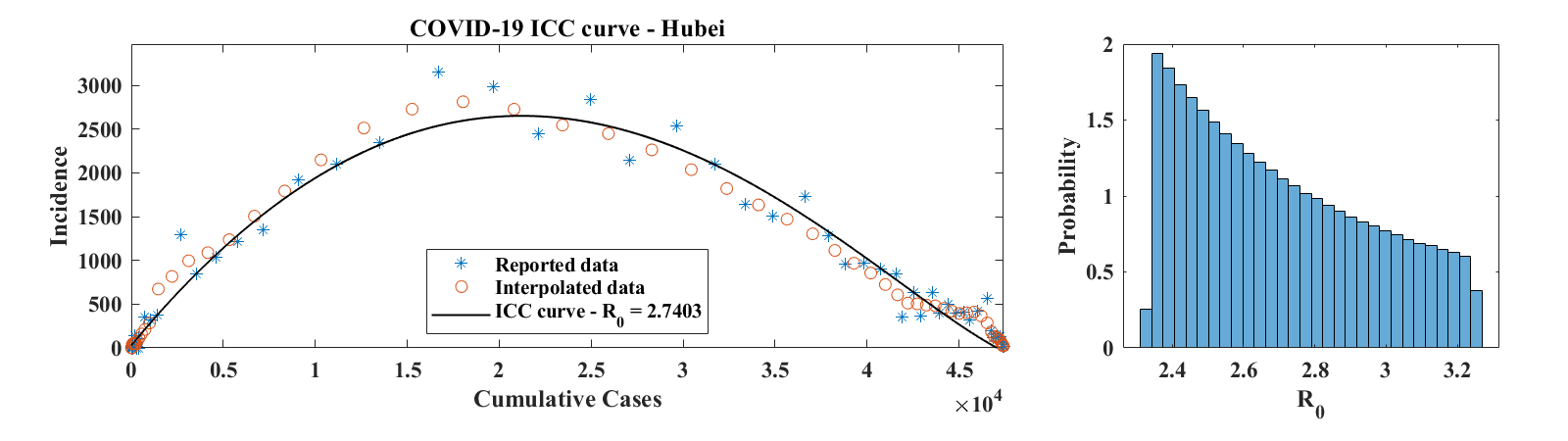
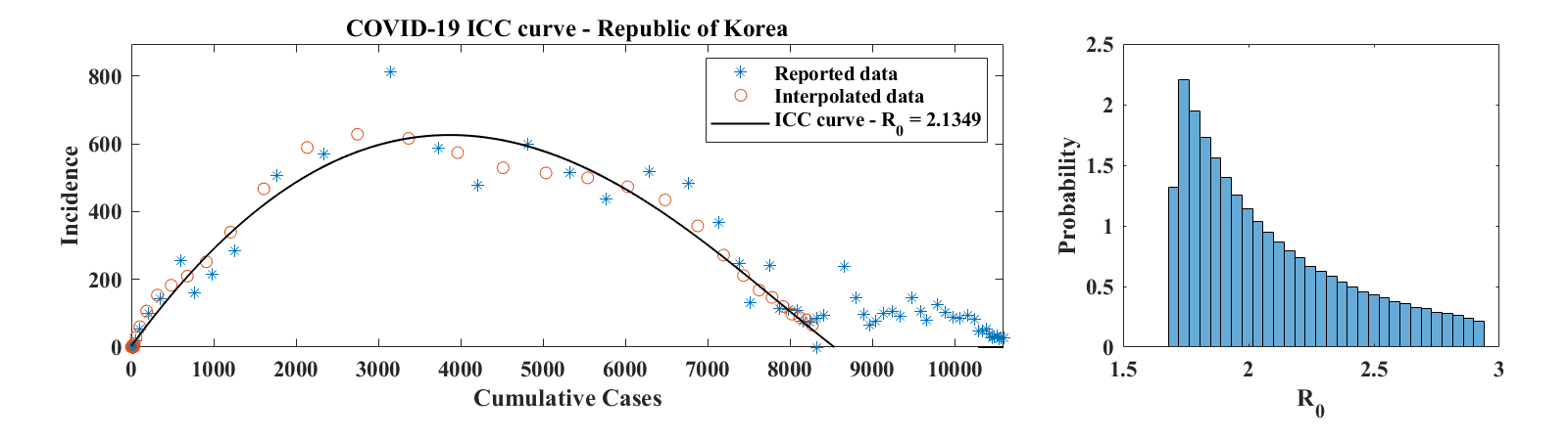
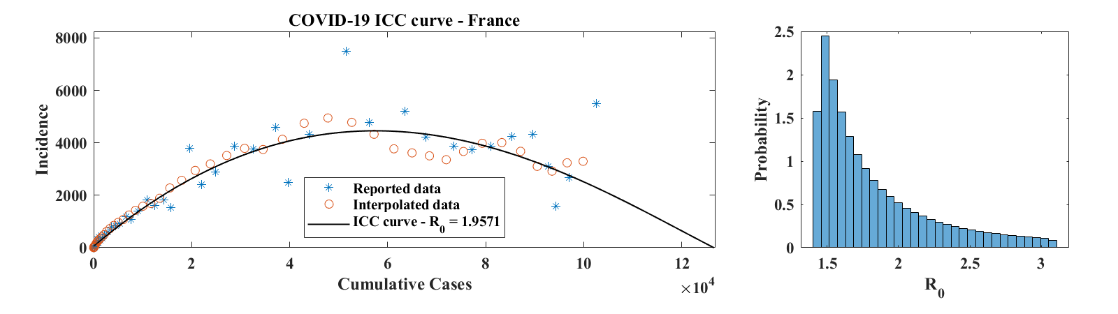
Figure 8 shows ICC curves for COVID-19 outbreaks in a few countries. The data was obtained from the World Health Organization daily situation reports [17] as well as from the Wuhan Health Municipal Commission [18]. For Hubei Province, only laboratory confirmed cases were used. Consequently, daily increment values for 2/17-19/2020 (days 65 to 67 in the data set, when China combined laboratory and clinically confirmed cases in its reports for a brief period of time) were set to half of the reported number of confirmed cases; the number of cumulative cases was then obtained by summing daily reports of laboratory confirmed cases. For the Republic of Korea, only the first 58 points in the data set were used, since they correspond to the first wave of the outbreak. The third example is for a country (France), where the outbreak was not over as of 4/15/2020. For each of these examples, we show the ICC curve for the set of parameters that best fits the interpolated data. The optimal values of are for Hubei Province, for the Republic of Korea, and for France. The corresponding optimal basic reproduction ratio values are for Hubei Province, for the Republic of Korea, and for France. A histogram of estimated values of , scaled to represent a probability distribution function, is shown in the right panel of each row of Figure 8. These were obtained as described above in the case of the outbreak in Mallorca, except that no Poisson-distributed noise was added to the data. This is because incidence values are generally large and that, as discussed in Section 3, the relative effect of the added noise is minimal, leading to a level of variability of that is insignificant compared to the effect of changing . Values of in the 2-3 range are consistent with early estimates of the basic reproduction ratio of COVID-19 published in the literature [19, 20].
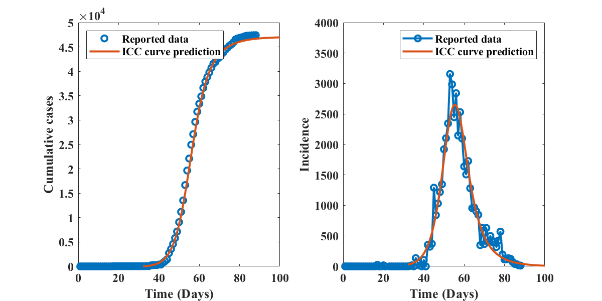
The time course of the COVID-19 outbreak in Hubei Province, as described by the SIR model with optimal parameters identified by the present method (, (), and ) is shown in Figure 9, together with the reported data. The solid curves are obtained by integration of the ICC curve, with initial conditions corresponding to day 10 of the outbreak, and alignment with the data at day 45. Similar plots for the other outbreaks discussed in this section are provided as supplementary material. The good visual agreement between simulation and data indicates that the SIR model, and therefore the ICC curve approach presented in this manuscript, are able to capture the overal dynamics of real-life outbreaks.
6. Conclusions
This article introduces a parameter estimation method for disease outbreaks that bypasses the numerical integration of epidemiological models. The approach relies on the use of ICC curves, also introduced here. ICC curves relate incidence to the cumulative number of cases and may be viewed as nonlinear transformations of the traditional epidemiological curves, in which the time variable is replaced by , a monotonically increasing but nonlinear function of time. For each single-wave outbreak, the ICC curve has a simple concave-down shape that crosses the horizontal axis at the origin and at the final value of .
The formulas presented in Section 2, which extend the parabolic approximation suggested in [1], are exact for the SIR model. The numerical experiments of Sections 3 and 4 show the method is robust to noise and may be used for parameter estimation as an outbreak unfolds, with the understanding that reasonably accurate estimates can only be reached shortly before, or after, incidence peaks. This is not a shortcoming of the present approach and was also observed in [11] when fitting synthetic prevalence time series.
Because of the simplicity of Equation 1, and the existence of a unique set of parameters that best fits any collection of data points, parameter distributions may be generated directly from epidemiological data. In the case of the SIR model, this methodology presents a fast and novel alternative to more traditional parameter estimation strategies, such as particle Makov Chain Monte Carlo methods (PMCMC; see [21] for a review). This may be beneficial in pandemic situations where epidemiological estimates need to be updated daily and in many locations simultaneously. For instance, recent work on COVID-19 data from Wuhan suggests that an SIR model can better capture the information contained in case reports than an SEIR model [22]. For more complex compartmental models, distributions generated by the present approach may be used as priors for PMCMC estimations of the contact and recovery rates of a disease.
When applying the proposed method to surveillance data, an estimate of may not always be available. The examples of Section 5 suggest that this parameter may be identified by optimizing the fit between the ICC curve and a smoothed and interpolated version of the reported data. However, any variability in the selected value of will be associated with variability in estimates of the basic reproduction number . Indeed, for an outbreak that has completed its course, any good fit of the reported data by an ICC curve will produce consistent values of , the final number of cases for the outbreak (see for instance the plots of Figure 8). Because of Equation 3, if is known, the estimated value of is only a function of . This uncertainty is inherent to the SIR model and cannot be avoided. The existence of a value of that best fits the data is encouraging, but more robust estimates are likely to be obtained if additional information is available. In the absence thereof, a range of values of close to the optimal value should be used to produce credible intervals for the basic reproduction ratio .
As previously mentioned, empirical (see [1]) and numerical observations by the author suggest the concave-down shape of the ICC curve is ubiquitous in outbreak data and in compartmental epidemiological models. It would therefore be interesting to explore methods which, like the discussion of Section 2, lead to exact formulations of ICC curves. In particular, knowledge of how model parameters affect the shape of ICC curves could provide simple means to visualize the consequences of mitigation effects. Combined with data assimilation, ICC curves may thus present a convenient paradigm for forecasting the course of an outbreak.
Declaration of competing interests.
No potential competing interest was reported by the author.
Data availability statement.
For codes and data sets used in this study, please see https://jocelinelega.github.io/EpiGro/.
Appendix A Critical parameter values
The function defined in Equation (4) has a unique extremizer given by the following expressions:
where
and we have used the notation
References
- [1] J. Lega and H.E. Brown, Data-driven outbreak forecasting with a simple nonlinear growth model, Epidemics 17, 19-26 (2016). http://dx.doi.org/10.1016/j.epidem.2016.10.002
- [2] W.O. Kermack and A.G. McKendrick, A contribution to the mathematical theory of epidemics, Proc. R. Soc. Lond. A115, 700–721 (1927). http://doi.org/10.1098/rspa.1927.0118
- [3] H.W. Hethcote, The Mathematics of Infectious Diseases, SIAM Review 42, 599-653 (2000). https://dx.doi.org/10.1137/S0036144500371907
- [4] O. Diekmann, J.A.P. Heesterbeek, and J.A.J. Metz, On the definition and the computation of the basic reproduction ratio in models for infectious diseases in heterogeneous populations, J. Math. Biol. 28, 365-382 (1990). https://doi.org/10.1007/BF00178324
- [5] P. van den Driessche, J. Watmough, Reproduction numbers and sub-threshold endemic equilibria for compartmental models of disease transmission, Mathematical Biosciences 180, 29-48 (2002). https://doi.org/10.1016/S0025-5564(02)00108-6
- [6] O. Diekmann, J.A.P. Heesterbeek, M.G. Roberts, The construction of next-generation matrices for compartmental epidemic models, J. R. Soc. Interface 7, 873-885 (2010). https://doi.org/10.1098/rsif.2009.0386
- [7] N.F. Britton, Essential Mathematical Biology, Springer Undergraduate Mathematics Series, 3rd Edition (2005), pages 90-93. https://www.springer.com/us/book/9781852335366
- [8] H. Miao, X. Xia, A.S. Perelson, H. Wu, On Identifiability of Nonlinear ODE Models and Applications in Viral Dynamics, SIAM Review 53, 3-39 (2011). https://doi.org/10.1137/090757009
- [9] N. Evans, L. White, M. Chapman, K. Godfrey, M. Chappell, The structural identifiability of the susceptible infected recovered model with seasonal forcing, Mathematical Biosciences 194, 175-197 (2005). https://doi.org/10.1016/j.mbs.2004.10.011
- [10] M.C. Eisenberg, S.L. Robertson, J.H. Tien, Identifiability and estimation of multiple transmission pathways in cholera and waterborne diseases, Journal of Theoretical Biology 324, 84-102 (2013). https://doi.org/10.1016/j.jtbi.2012.12.021
- [11] N. Tuncer, T.T. Le, Structural and practical identifiability analysis of outbreak models, Mathematical Biosciences 299, 1-18 (2018). https://doi.org/10.1016/j.mbs.2018.02.004
- [12] K. Roosa, G. Chowell, Assessing parameter identifiability in compartmental dynamic models using a computational approach: Application to infectious disease transmission models, Theoretical Biology and Medical Modelling 16, 1 (2019). https://doi.org/10.1186/s12976-018-0097-6
- [13] G. Chowell, Fitting dynamic models to epidemic outbreaks with quantified uncertainty: A primer for parameter uncertainty, identifiability, and forecasts, Infectious Disease Modelling 2, 379-398 (2017). http://dx.doi.org/10.1016/j.idm.2017.08.001
- [14] A.A. King, M. Domenech de Celles, F.M.G. Magpantay, P. Rohani, Avoidable errors in the modelling of outbreaks of emerging pathogens, with special reference to Ebola, Proc. R. Soc. B 282, 20150347 (2015). https://dx.doi.org/10.1098/rspb.2015.0347
- [15] Maple 2018. Maplesoft, a division of Waterloo Maple Inc., Waterloo, Ontario.
- [16] M.A. Luque Fernández, A. Galmés Truyols, D. Herrera Guibert, G. Arbona Cerdá, F. Sancho Gayá, Cohort study of an outbreak of viral gastroenteritis in a nursing home for elderly, Majorca, Spain, February 2008, Euro Surveill. 13(51), pii=19070 (2008). https://www.eurosurveillance.org/content/10.2807/ese.13.51.19070-en
- [17] WHO Coronavirus disease (COVID-2019) situation reports. https://www.who.int/emergencies/diseases/novel-coronavirus-2019/situation-reports
- [18] Wuhan Health Municipal Commission. http://wjw.wuhan.gov.cn/. The page that reported COVID-19 data, http://wjw.wuhan.gov.cn/front/web/list2nd/no/710 has now been removed.
- [19] J.T. Wu, K. Leung, G.M. Leung, Nowcasting and forecasting the potential domestic and international spread of the 2019-nCoV outbreak originating in Wuhan, China: a modelling study, Lancet 395, 689–97 (2020). https://doi.org/10.1016/S0140-6736(20)30260-9
- [20] See also the MIDAS Network dashboard, which lists estimates of in a range of preprints. https://midasnetwork.us/covid-19/
- [21] A. Endo, E. van Leeuwenb, M. Baguelin, Introduction to particle Markov-chain Monte Carlo for disease dynamics modellers, Epidemics 29, 100363 (2019). https://doi.org/10.1016/j.epidem.2019.100363
- [22] W.C. Roda, M.B. Varughese, D. Han, M.Y. Li, Why is it difficult to accurately predict the COVID-19 epidemic?, Infectious Disease Modeling 5, 271-291 (2020). https://doi.org/10.1016/j.idm.2020.03.001