Parameter Identification with Finite-Convergence Time Alertness Preservation*

Romeo Ortega¹, Alexey Bobtsov² and Nikolay Nikolaev² *This paper is partially supported by the Ministry of Science and Higher Education of Russian Federation, passport of goszadanie no. 2019-0898.¹Romeo Ortega is with Departamento Académico de Sistemas Digitales, ITAM, Ciudad de México, México. romeo.ortega@itam.mx²Alexey Bobtsov and Nikolay Nikolaev are with ITMO University, Kronverkskiy av. 49, St. Petersburg, 197101, Russia. bobsov@mail.ru and nikona@yandex.ru

Abstract

In this brief note we present two new parameter identifiers whose estimates converge in finite time under weak interval excitation assumptions. The main novelty is that, in contrast with other finite-convergence time (FCT) estimators, our schemes preserve the FCT property when the parameters change. The previous versions of our FCT estimators can track the parameter variations only asymptotically. Continuous-time and discrete-time versions of the new estimators are presented.

I PARAMETER ESTIMATORS WITH ALERTNESS-PRESERVING FINITE-CONVERGENCE TIME

The objective of this work is to propose continuous-time (CT) and discrete-time (DT) on-line estimators of the parameters $\theta\in\mathbb{R}^{q}$ of a linear regression equation (LRE) of the form

y=\phi^{\top}\theta,

(1)

from the measurable quantities $y$ and $\phi$ . The estimators should satisfy three specifications

S1

Convergence of the estimates should be achieved in finite-time.
S2

Convergence is ensured under weak interval excitation (IE) conditions [4].
S3

The estimator should preserve its alertness to be able to estimate—still with FCT—future variations of the unknown parameters.

Instrumental to solve this problem is the use of the dynamic regressor extension and mixing (DREM) procedure proposed in [1]. In particular, we adapt the FCT-DREM estimator proposed in [6] to incorporate the new feature of FCT alertness preservation (AP). A CT version of such an scheme was reported in [7, Section V], in this note we give a DT version of it.

An early variation of the least-squares method, that converges in finite time, was proposed 32 years ago. Similarly to more recent FCT estimators [2, 3, 9] in its initial stage the algorithm is akin to an off-line estimator, which involves a numerically sensitive matrix inversion and, as it converges to a standard least-squares, loses its alertness. For the sake of completeness we present comparative simulations of the proposed estimator with the FCT estimator reported in [12], which relies on the injection of high-gain via the use of fractional powers and/or relays in the estimator dynamics. See also [8, 11] where a similar high-gain approach is adopted.

Notation. $\mathbb{R}_{>0}$ , $\mathbb{R}_{\geq 0}$ , $\mathbb{Z}_{>0}$ and $\mathbb{Z}_{\geq 0}$ denote the positive and non-negative real and integer numbers, respectively. Continuous-time (CT) signals $s:\mathbb{R}_{\geq 0}\to\mathbb{R}$ are denoted $s(t)$ , while for discrete-time (DT) sequences $s:\mathbb{Z}_{\geq 0}\to\mathbb{R}$ we use $s(k):=s(kT_{s})$ , with $T_{s}\in\mathbb{R}_{>0}$ the sampling time. When a formula is applicable to CT signals and DT sequences the time argument is omitted.

II FCT ESTIMATORS: FORMULATION FROM SCALAR LRES VIA DREM

As it has been widely documented the powerful DREM estimator design procedure [1] allows us to generate, from the $q$ -dimensional LRE (1), $q$ -scalar LREs of the form

{\cal Y}_{i}=\Delta\theta_{i},\quad i\in\bar{q}:=\{1,2,\dots,q\}

(2)

where $\Delta$ is the determinant of an extended regressor matrix. In the remaining of the note, we will use this simple scalar LREs to design the AP-FCT parameter estimator.

II-A CT FCT-DREM

The following CT FCT-DREM estimator was reported in [6] and, as it constitutes the basis of our new AP-FCT, we repeat it for ease of reference. Also, to make the note self-contained we give a brief summary of the proof, referring the interested reader to [6] for further details.

Proposition 1

Consider the scalar CT LREs (2) and the gradient-descent estimators¹¹1In the sequel, the quantifier $i\in\bar{q}$ is omitted for brevity.

\dot{\hat{\theta}}_{i}(t)=\gamma_{i}\Delta(t)[{\cal Y}_{i}(t)-\Delta(t)\hat{\theta}_{i}(t)],

(3)

with $\gamma_{i}>0$ . Define the FCT estimate

\hat{\theta}_{i}^{\tt FCT}(t):={1\over 1-w^{\tt c}_{i}(t)}[\hat{\theta}_{i}(t)-w_{i}^{\tt c}(t)\hat{\theta}_{i}(0)],

(4)

where $w_{i}^{\tt c}(t)$ is defined via the clipping functions

w_{i}^{\tt c}(t)=\left\{\begin{array}[]{lcr}\mu_{i}\;\;\;\mbox{if}\;\;\;\;\;w_{i}(t)\geq\mu_{i}\\ \\ w_{i}(t)\;\;\mbox{if}\;\;\;\;\;w_{i}(t)<\mu_{i},\end{array}\right.

(5)

$\mu_{i}\in(0,1)$ are designer chosen parameters, and $w_{i}(t)$ is given by

\dot{w}_{i}(t)=-\gamma_{i}\Delta^{2}(t)w_{i}(t),\;w_{i}(0)=1.

(6)

Assume there exists a time $t_{i}^{c}>0$ such that the IE condition [4]

\int^{t_{i}^{c}}_{0}\Delta^{2}(\tau)d\tau\geq-\frac{1}{\gamma_{i}}\ln(1-\mu_{i}),

(7)

is satisfied. Then,

\hat{\theta}_{i}^{\tt FCT}(t)=\theta_{i},~~\forall t>t_{i}^{c},

(8)

that is, the estimator has the feature of FCT.

Proof:

Define the parameter errors $\tilde{\theta}_{i}:=\hat{\theta}_{i}-\theta_{i}.$ The scalar error equations are given by

\dot{\tilde{\theta}}_{i}(t)=-\gamma_{i}\Delta^{2}(t)\tilde{\theta}_{i}(t),

whose explicit solution is

\displaystyle{\tilde{\theta}_{i}(t)=e^{-\gamma_{i}\int_{0}^{t}\Delta^{2}(s)ds}\tilde{\theta}_{i}(0).}

(9)

Now, notice that the solution of (6) is

w_{i}(t)=e^{-\gamma_{i}\int_{0}^{t}\Delta^{2}(s)ds}.

The key observation is that, using the equation above in (9), and rearranging terms we get that

[1-w_{i}(t)]\theta_{i}=\hat{\theta}_{i}(t)-w_{i}(t)\hat{\theta}_{i}(0).

(10)

Now, observe that $w_{i}(t)$ is a non-increasing function and, under the interval excitation assumption (7), we have that

w^{\tt c}_{i}(t)=w_{i}(t)<\mu_{i}<1,\;\forall t\geq t_{c},

(11)

Clearly, (10) and (11) imply that

\frac{1}{1-w_{c}(t)}\left[\hat{\theta}(t)-w_{c}(t)\hat{\theta}(0)\right]=\theta,\;\forall t>t_{c},

completing the proof. $\Box\Box\Box$

II-B DT FCT-DREM

In [6, Proposition 2] a DT DREM estimator was reported. We give below an FCT-version of this scheme and give a brief summary of the proof.

Proposition 2

Consider the scalar DT LREs defined by (2) with the DT gradient-descent estimator

\hat{\theta}_{i}(k+1)=\hat{\theta}_{i}(k)+\frac{{\Delta}(k)}{c_{i}+{\Delta}^{2}(k)}\left[{{\cal Y}}_{i}(k+1)-{\Delta}(k)\hat{\theta}_{i}(k)\right]

(12)

with positive constants $c_{i}$ . Define the dynamic extension

w_{i}(k+1)=\frac{c_{i}}{c_{i}+{\Delta}^{2}(k)}w_{i}(k),\;\;w_{i}(0)=1.

(13)

and the clipping function

w_{i}^{c}(k)=\left\{\begin{aligned} &\rho_{i}&\mbox{if $w_{i}(k)\in[\rho_{i},1]$}\\ &\\ &w_{i}(k)&\mbox{if $w_{i}(k)\in[0,\rho_{i})$},\end{aligned}\right.

(14)

where $\rho_{i}\in(0,1)$ are designer chosen constants. Assume there exists a $k_{i}^{c}\in(0,\infty)$ such that the IE condition

\prod_{i=0}^{k_{i}^{c}}\left[\frac{c_{i}}{c_{i}+{\Delta}^{2}(i)}\right]<\rho_{i},

(15)

is satisfied. Then,

\hat{\theta}_{i}^{\tt FCT}(k):={1\over 1-w_{i}^{c}(k)}[\hat{\theta}_{i}(k)-w_{i}^{c}(k)\hat{\theta}_{i}(0)],

(16)

ensures

{\hat{\theta}}_{i}^{\tt FCT}(k)=\theta_{i},\;\forall k\geq k_{i}^{c}.

Proof:

From, (2) and (12) we get the parameter error equation

\tilde{\theta}_{i}(k+1)=\frac{c_{i}}{c_{i}+{\Delta}^{2}(k)}\tilde{\theta}_{i}(k)

(17)

whose explicit solution satisfies

\tilde{\theta}_{i}(k)=\psi_{i}(k)\tilde{\theta}_{i}(0),

(18)

where, for ease of future reference, we defined the scalar sequence

\psi_{i}(k):=\prod_{i=0}^{k}\left[\frac{c_{i}}{c_{i}+{\Delta}^{2}(i)}\right]

(19)

The solution of (13) is given by

w_{i}(k)=\psi_{i}(k),

(20)

whose replacement in (18) yields

\tilde{\theta}_{i}(k)=w_{i}(k)\tilde{\theta}_{i}(0).

Using the definition of the parameter error and rearranging terms we get that

[1-w_{i}(k)]\theta_{i}=\hat{\theta}_{i}(k)-w_{i}(k)\hat{\theta}_{i}(0).

(21)

According to (14) we have that, under the assumption (15), $w_{i}(k)<\rho_{i}<1$ for all $k\geq k_{i}^{c}$ , Consequently, for $k\geq k_{i}^{c}$ we can write

\theta_{i}={1\over 1-w_{i}(k)}[\hat{\theta}_{i}(k)-w_{i}(k)\hat{\theta}_{i}(0)].

The proof is completed, from (16), noting that $w_{i}(k)=w_{i}^{c}(k)$ for all $k\geq k_{i}^{c}$ . $\Box\Box\Box$

III NEW ESTIMATOR WITH FCT ALERTNESS PRESERVATION

There are two practical problems with the approach described above. First, the estimates at the current time are reconstructed from the knowledge of the initial estimate $\hat{\theta}_{i}(0)$ , complicating the task of tracking variations of the true parameters after convergence of the estimates. Second, independently of the behaviour of $\Delta$ , the functions $w_{i}$ are monotonically non-increasing and converge to zero if $\Delta$ is not square summable (or integrable). In this case, $\hat{\theta}_{i}^{\tt FCT}\to\hat{\theta}_{i}$ , and the FCT estimator converges to a standard gradient, losing its FCT feature. Therefore, to keep the FCT alertness of the estimator, i.e., to track parameter variations in finite-time upon the arrival of new excitation, it is necessary to reset the estimators—a modification that is always problematic to implement. A typical procedure is the so-called covariance resetting for least-squares algorithms, see [10, Section 2.4.2].

These drawbacks can be overcome with the new FCT-DREM estimators proposed below.

III-A CT FCT-DREM with alertness preservation

For the sake of brevity, we present only the derivation of a relation similar to (10), from which we can easily construct the FTC estimator and prove that the new FTC estimator does not converge to the gradient one.

Proposition 3

Fix $T_{\tt D}\in\mathbb{R}_{>0}$ and define

\dot{w}_{i}^{\tt D}(t)=-\gamma_{i}\left[\Delta^{2}(t)-\Delta^{2}(t-T_{\tt D})\right]w_{i}^{\tt D}(t),\;w^{\tt D}_{i}(0)=1.

(22)

Then,

\left[1-w_{i}^{\tt D}(t)\right]\theta_{i}=\hat{\theta}_{i}(t)-w_{i}^{\tt D}(t)\hat{\theta}_{i}(t-T_{\tt D}).

(23)

Moreover, $w_{i}^{\tt D}(t)$ is bounded away from zero.

Proof:

Without loss of generality we assume that $\Delta(t-T_{\tt D})=0$ for $t<T_{\tt D}$ . Then, the solution of (22) is

w_{i}^{\tt D}(t)=e^{-\gamma_{i}\int_{t-T_{\tt D}}^{t}\Delta^{2}(s)ds}.

(24)

From (24), and the fact that

\int_{t-T_{\tt D}}^{t}\Delta^{2}(s)ds\leq\Delta^{2}_{\max}T_{\tt D},

where $\Delta_{\max}\geq\|\Delta(t)||_{\infty}$ , we conclude that

w_{i}^{\tt D}(t)\geq e^{-\gamma_{i}\Delta^{2}_{\max}T_{\tt D}}>0.

Now, from the solution of the parameter error equation (9) in the interval $[t-T_{\tt D},t]$ we get

\tilde{\theta}_{i}(t)=e^{-\gamma_{i}\int_{t-t_{\tt D}}^{t}\Delta^{2}(s)ds}\tilde{\theta}_{i}(t-T_{\tt D}).

Hence, $\tilde{\theta}_{i}(t)=w_{i}^{\tt D}(t)\tilde{\theta}_{i}(t-T_{\tt D}).$ The proof of the claim is established rearranging the terms of the equation above.

$\Box\Box\Box$

Remark 1

It is important to note that when $\Delta(t)$ decreases—that is, when we loose excitation— $w_{i}^{\tt D}(t)$ grows towards one, and the alertness in not lost. On the other hand, when new excitation arrives and $\Delta(t)$ grows, then $w_{i}^{\tt D}(t)$ decays and the FCT condition $w_{i}^{\tt D}(t)<\mu_{i}$ is satisfied. In this way, the new FTC estimator preserves its FTC property if the parameters change. This fact is illustrated in the simulations of Section IV. Notice also that, in contrast with the FCT estimator of Proposition 1, where the calculation of the $\hat{\theta}^{\tt FCT}_{i}$ in (4) is done using the initial parameter estimate $\hat{\theta}_{i}(0)$ , the FCT reconstruction of the estimated parameter is done in (23) using the estimate at time $t-T_{\tt D}$ , that is, $\hat{\theta}_{i}(t-T_{\tt D})$ .

Remark 2

For the new FTC DREM estimator the interval excitation inequality becomes the existence of a time $t_{i}^{c}\geq T_{\tt D}$ such that

\int^{t_{i}^{c}}_{t_{i}^{c}-T_{\tt D}}\Delta^{2}(s)ds\geq-\frac{1}{\gamma_{i}}\ln(1-\mu_{i}).

(25)

Recalling (24), it has the same interpretation as (7).

III-B DT FCT-DREM with alertness preservation

Similarly to the CT case, for the sake of brevity, we present only the derivation of a relation similar to (21), from which we can easily construct the FTC estimator and prove that the new FTC estimator does not converge to the gradient one.

Proposition 4

Fix a positive integer ${\tt d}$ . Consider the DT, scalar LRE (2) and the gradient parameter update (12) with the dynamic extension (13) and the sequence

Then,

[1-w_{i}^{\tt d}(k)]\theta_{i}=\hat{\theta}_{i}(k)-w_{i}^{\tt d}(k)\hat{\theta}_{i}(k-{\tt d}).

Proof:

First, we make the observation that, for all finite $k$ , the sequence $w_{i}(k)$ is bounded away from zero. Replacing the solution of $w_{i}(k)$ —given by (19) and (20)—in (LABEL:wdk) it is clear that

w_{i}^{\tt d}(k)=\prod_{i=k-{\tt d}}^{k}\left[\frac{c_{i}}{c_{i}+{\Delta}^{2}(i)}\right]

Hence, replacing the equation above in (18) we have that

\tilde{\theta}_{i}(k)=w_{i}^{\tt d}(k)\tilde{\theta}_{i}(k-{\tt d}).

The proof is completed rearranging the terms of the identity above. $\Box\Box\Box$

Remark 3

It is clear that the same behavior that is indicated in Remark 1 regarding the CT version is observed in this DT one—explaining the important FCT-AP property.

IV SIMULATIONS

In this section we present simulations illustrating the results of Propositions 1-4 for a single parameter. Moreover, for the sake of comparison, we show some simulation results of the high-gain FCT estimator proposed in [12].

IV-A CT FCT-DREM with alertness preservation

In this subsection we compare the FCT DREM of Proposition 1 and the new FCT DREM of Proposition 3. The objective of the simulation is to prove that the new FTC DREM is able to react when new excitation arrives. This is in contrast with the old FCT DREM estimator that, since $w_{i}(t)\to 0$ , converges to the gradient estimator and loses its FTC alertness property.

We consider two scenarios: with and without excitation in $\Delta(t)$ . For the first case we consider the PE signal $\Delta(t)=\sin({\pi\over 10}t)$ , and for the second one $\Delta(t)=\frac{1}{\sqrt{t+1}}$ . Note that in the second case $\Delta(t)\to 0$ , hence it is not PE. However, $\Delta(t)\not\in\mathcal{L}_{2}$ , hence it satisfies the conditions for convergence of the DREM estimator [1, 7].

To illustrate the FTC tracking capabilities of the estimators the unknown parameter $\theta$ is time-varying and given by

\theta(t)=\begin{cases}10\text{ for }0\leq t<10,\\ 15\text{ for }10\leq t<20,\\ 15-0.5(t-20)\text{ for }20\leq t<30,\\ 10\text{ for }t>30,\\ \end{cases}

i.e., it starts at $10$ , jumps to $15$ at $t=10$ , and then linearly returns to $10$ .

For the simulations we set $\gamma=2$ , $\mu=0.98$ , and $T_{\tt D}=0.2$ . These parameters have been chosen such that the transients of both FCT estimators coincide in the ideal case when $\theta$ is constant and the system is excited.

The transient of the estimators for $\Delta(t)=\sin({\pi\over 10}t)$ are given in Fig. 1, where we plot the time-varying parameter $\theta$ , the gradient estimate $\hat{\theta}^{grad}(t)$ , as well as the old and the new FCT estimates, denoted in the plots as $\hat{\theta}^{\tt FCT}(t)$ and $\hat{\theta}^{\tt FCT-D}(t)$ , respectively. We observe that, as expected, in the time interval $[0,10]$ both FCT estimators are overlapped and converge in finite time, while the gradient converges only asymptotically. The difference between the old FCT estimator and the new one is clearly appreciated in the time interval $[10,20]$ , where we see that the new FCT estimator tracks the parameter variation in finite time, while the old one—now glued to the gradient—only does it asymptotically.

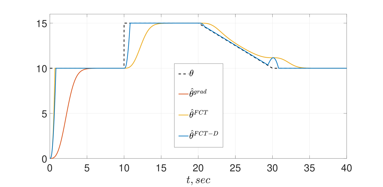
Refer to caption — Figure 1: Transients of the CT parameter estimates with $\Delta(t)=\sin({\pi\over 10}t)$ .

The behavior of the CT estimators for $t\in[20,40]$ shows that, as predicted by the theory, the old FCT behaves as the gradient estimator and their trajectories coincide. On the other hand, the new estimator preserves FCT alertness after the first parameter jump and achieves fast tracking of the linearly time-varying $\theta(t)$ . We also observe in the figure a blip in the estimates at $t=30$ that coincides with the time of freezing of the true parameter.

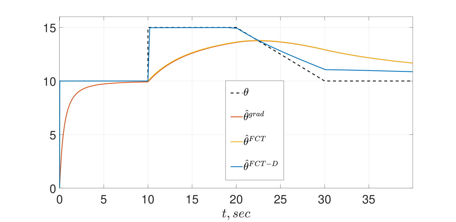
For the non-PE case of $\Delta=1/\sqrt{t+1}$ , the transients of the CT estimators are given in Fig. 2. We observe that both FCT estimators, again, essentially coincide in the first few seconds and converge in finite time, while the gradient does it only asymptotically. After the first parameter change at $t=10$ the old FTC and the gradient coincide, while the new FCT manages to track in finite time the parameter jump. However, during the ramp parameter change—because of the lack of excitation—neither one of the estimators can track the parameter variation but the new FCT estimator performs much better.

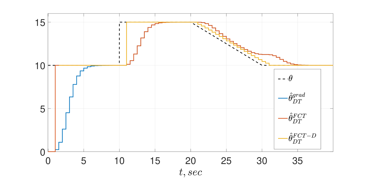
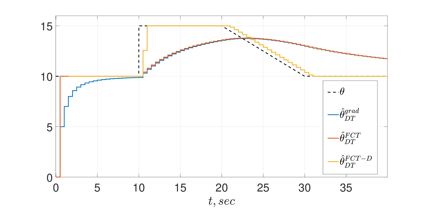
IV-B DT FCT-DREM with alertness preservation

In this subsection we present the simulation results for the DT estimators of Propositions 2 and 4. The estimator gains were set to $\gamma=2$ , $c=1$ , $d=1$ , $T_{\tt D}=1$ and $T=0.5$ .

The same simulation scenario of the CT schemes given above is reproduced here and the transient behaviors are shown in Figs. 3 and 4. Essentially the same remarks made for the CT schemes of the previous subsection are applicable in the DT case.

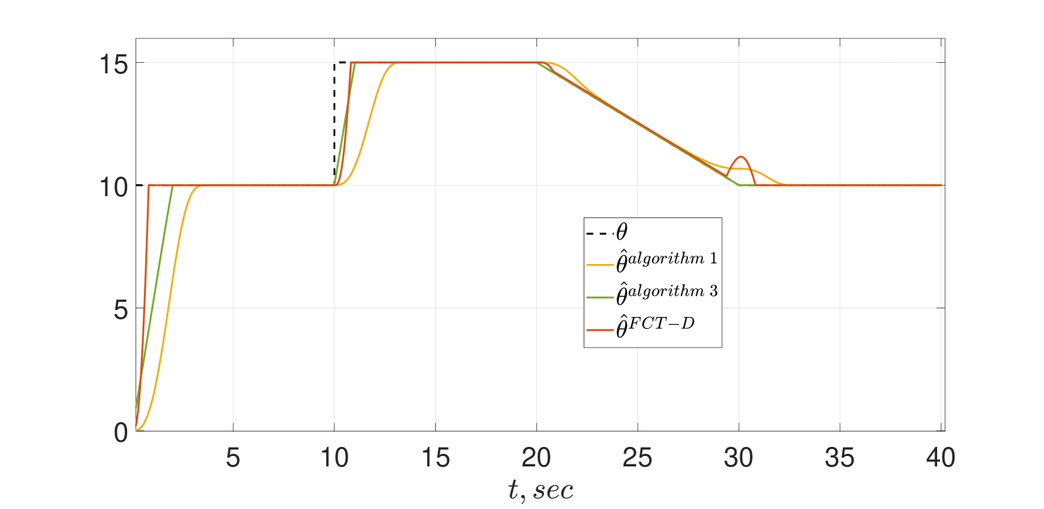
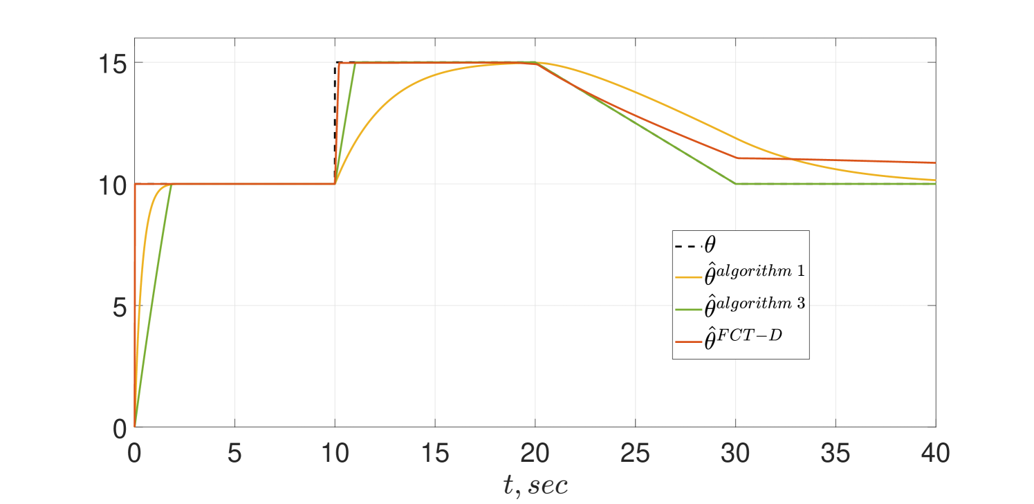
IV-C Comparison of the CT FCT-DREM with two schemes of [12]

Now, we compare the FCT-D algorithm with two of the schemes proposed in [12]. Namely,

i)

Algorithm 1

$\displaystyle\dot{\hat{\theta}}(t)=\gamma\Delta(t)\lceil{\cal Y}(t)-\Delta(t)\hat{\theta}(t)\rfloor^{\alpha}$ (26)

where $\gamma>0$ and $\alpha\in\left[0,1\right)$ .

ii)

Algorithm 3

\displaystyle\dot{\hat{\theta}}(t)=\gamma\mbox{sign}(\Delta(t))\lceil{\cal Y}(t)-\Delta(t)\hat{\theta}(t)\rfloor^{\frac{\left|\Delta(t)\right|}{\varsigma\Delta_{max}}}

(27)

where $\gamma>0$ , $\varsigma>1$ , $\Delta_{max}=\max_{t\in\left[-T^{0},T^{0}+T\right]\left|\Delta(t)\right|}$ for given $T^{0}\in\mathbb{R}_{+}$ and $\hat{\theta}(t_{0})=0$ .

It should be underscored in [12] a third estimator was also proposed but this scheme is not well-defined when $\Delta(t)=0$ and could not be simulated.

For the simulation of the CT FCT-D we set $\gamma=2$ , $\mu=0.98$ , and $T_{\tt D}=0.2$ , while for Algorithm 1 (26) we set $\gamma=5$ and $\alpha=0.75$ . and for Algorithm 3 (27) we set $\gamma=5$ , $\varsigma=2$ .

The same simulation scenario of the CT schemes given in Subsection IV-A is reproduced here and the transient behaviors are shown in Figs. 5 and 6. As shown in the figures Algorithm 3 indeed achieves FCT and preserves its alertness. However, in spite of the theoretical analysis reported in [12] the estimator of Algorithm 1 tracks only asymptotically.

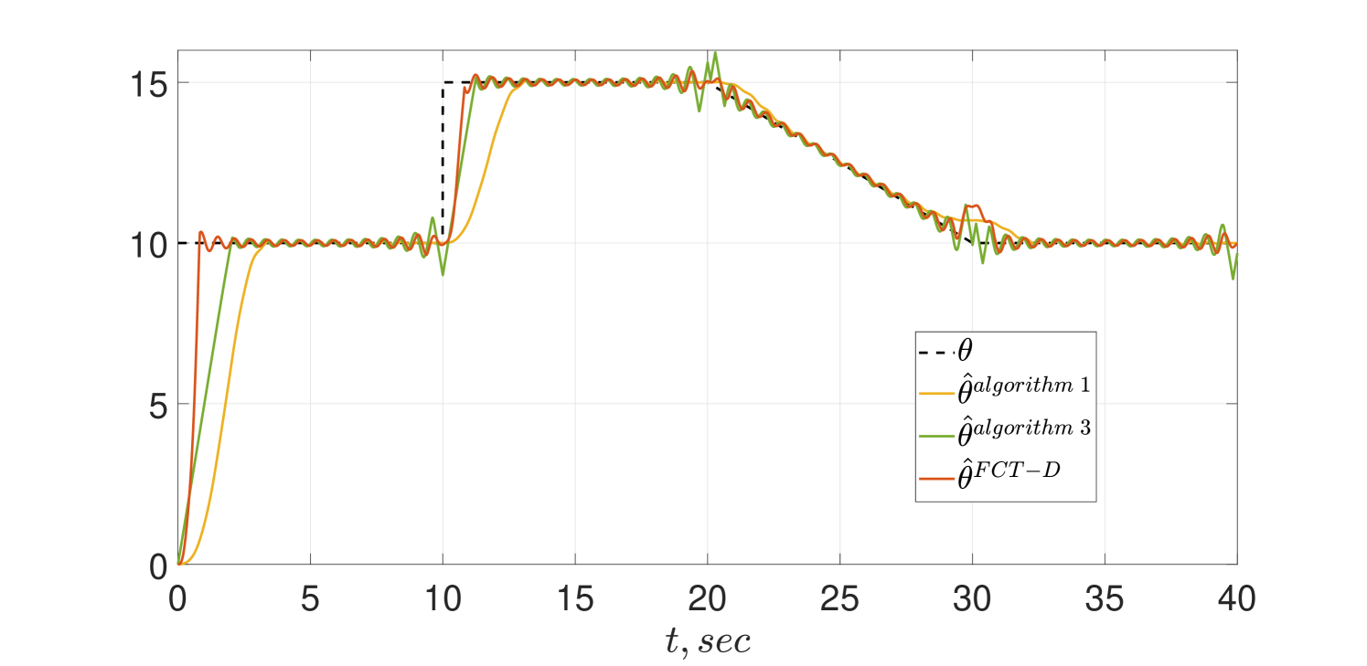
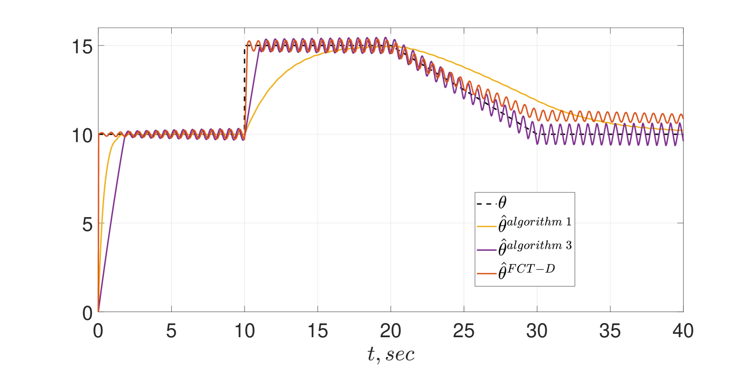
To test the sensitivity of the algorithms to the presence of noise, we repeated the simulations adding a signal $0.1\sin(10t)$ to the measurement ${\cal Y}(t)$ . The results of the simulations are shown in Figs. 7 and 8. Interestingly, the behavior of Algorithm 1 does no seem to be affected by the noise—but, as before, the tracking is only asymptotic. For the PE case of Fig 7 we see only a minor performance degradation due to the noise in all schemes that is further degraded for the non-PE case of Fig 8.

V CONCLUSIONS

We have presented two new FCT-DREM parameter estimators with enhanced performance—in particular, with respect to their ability to track parameter variations in finite-time. CT and DT versions of the new estimators are given. The performance improvement of the proposed schemes was illustrated with representative simulations.

References

[1] S. Aranovskiy, A. Bobtsov, R. Ortega and A. Pyrkin, Performance enhancement of parameter estimators via dynamic regressor extension and mixing, IEEE Transactions on Automatic Control, vol. 62, no. 7, pp. 3546-3550, 2017.
[2] N. Cho, H. Shin, Y. Kim and A. Tsourdos, Composite MRAC with parameter convergence under finite excitation, IEEE Trans. Automatic Control, vol. 63, no. 3, pp. 811-818, 2018.
[3] G. Chowdhary, T. Yucelen, M. Mhlegg and E. Johnson, Concurrent learning adaptive control of linear systems with exponentially convergent bounds, Int. J. on Adaptive Control and Signal Processing, vol. 27, no. 4, pp. 280-301, 2013.
[4] G. Kreisselmeier and G. Rietze-Augst, Richness and excitation on an interval—with application to continuous-time adaptive control, IEEE Trans. Automatic Control, Vol. 35, No. 2, pp. 165-171, 1990.
[5] R. Ortega, An on-line least-squares parameter estimator with finite convergence time, Proc. of the IEEE, vol. 76, no. 7, 1988.
[6] R. Ortega, D. Gerasimov, N. Barabanov and V. Nikiforov, Adaptive control of linear multivariable systems using dynamic regressor extension and mixing estimators: Removing the high-frequency gain assumption, Automatica, (doi.org/10.1016/j.automatica.2019.108589.).
[7] R. Ortega, S. Aranovskiy, A. A. Pyrkin, A. Astolfi and A. A. Bobtsov, New results on parameter estimation via dynamic regressor extension and mixing: continuous and discrete-time cases, IEEE Transactions on Automatic Control, (10.1109/TAC.2020.3003651), 2020.
[8] H. Rios, D. Efimov, J. Moreno and W. Perruquetti, Time-varying parameter identification algorithms: finite and fixed-time convergence, IEEE Transactions on Automatic Control, vol. 62, no. 7, pp. 3671-3678, 2017.
[9] S.B. Roy and S. Bhasin and I.N. Kar, Combined MRAC for unknown MIMO LTI systems with parameter convergence, IEEE Transactions on Automatic Control, vol. 63, no. 1, pp. 283-290, 2018.
[10] S. Sastry and M. Bodson, Adaptive Control: Stability, Convergence and Robustness, Prentice-Hall, New Jersey, 1989.
[11] J. Wang, D. Efimov, S. Aranovskiy and A. Bobtsov, Fixed-time estimation of parameters for non-persistent excitation, European Journal of Control, vol. 55, pp. 24-32, 2020
[12] Wang, Jian, Denis Efimov, and Alexey A. Bobtsov. On robust parameter estimation in finite-time without persistence of excitation. IEEE Transactions on Automatic Control vol. 65 N. 4 pp. 1731-1738, 2020.

TABLE I: List of Acronyms

AP	Alertness preservation
CT	Continuous-time
DREM	Dynamic regressor extension and mixing
DT	Discrete-time
FCT	Finite-convergence time
IE	Interval excitation
LRE	Linear regressor equation