Particle Motion in Rapidly Oscillating Potentials: The Role of the Potential’s Initial Phase

The theoretical study of the dynamics of a particle moving in a rapidly oscillating potential has been an active field of research for the past 50 years Kap51 ; LanLif76 ; GapMil58 ; Deh67 ; PerRic82 ; NadOks86 ; Com86 ; CooSha85 ; GroRak88 ; Fis03 . In 1951, Kapitza showed that rapidly oscillating potentials can have a stabilizing effect on dynamical systems Kap51 , which he demonstrated utilizing an inverted pendulum whose suspension point was forced to oscillate vertically. For high enough frequencies and large enough amplitudes of this oscillation the upwards position of the pendulum becomes stable. Kapitza showed that the pendulum feels a time independent effective potential that has a local minimum at the pendulum’s upwards position and thus imparts stability upon it. This phenomenon has since been termed “dynamic stabilization”. In 1958, Paul used the principle of dynamic stabilization to trap charged ions by alternating electric fields Pau90 . Ions trapped within a Paul trap have and continue to be used in the development of frequency standards, other fundamental measures BlaGil92 and quantum information CirZol95 .
In order to grasp all the possible applications that are offered by atoms which are trapped by rapidly oscillating potentials, a descriptive theory of their dynamics is indispensable. For the motion of ions in a Paul trap such a theory is given by Mathieu’s theory, which provides the exact solution of the ion’s classical equations of motion in terms of the tabulated Mathieu functions Pau90 ; LeiBla03 ; MajGhe04 . However, this theory is restricted to potentials of harmonic shape which are oscillated sinusoidally only. Besides this, Mathieu’s theory does not raise intuition regarding the atom’s dynamics hindering the discovery of new phenomena. For these purposes, Kapitza’s theory of the effective potential has thus far been suitable, sufficiently explaining the stabilization of the inverted pendulum Kap51 . This theory has since been generalized to arbitrary rapidly oscillating potentials LanLif76 ; Fis03 and extended to quantum mechanics CooSha85 ; GroRak88 ; Fis03 .
In this paper, we describe a different phenomenon, which illustrates that the motion of a particle trapped by a rapidly oscillating potential with a vanishing time average significantly depends on the potential’s initial phase for arbitrarily high frequencies of its oscillation. We discover that this phenomenon cannot be explained by the effective potential theory which we find to be incomplete. Therefore, we derive the necessary completion in order to describe this phenomenon.
Kapitza’s effective potential theory is based on a separation of the particle’s motion into a slow and a fast changing part. For high frequencies of the potential’s oscillation this separation can be performed in such a way that the slow part is governed by a time independent potential while the fast part has a vanishing time average and a negligible amplitude. In Kapitza’s theory it is concluded that the particle’s real motion is approximately described by its slow part, such that the real motion can be obtained by replacing its time dependent equation of motion by the time independent equation of motion of the slow part. However, doing so requires replacing the particle’s initial conditions by the corresponding initial conditions of the slow part. If these two sets of initial conditions significantly differ from each other, the replacement of the initial conditions is a crucial point in the determination of the real motion. In the context of adiabatic elimination a significant difference between the initial conditions of the full problem and the model problem is called an “initial slip” GeiTit83 ; HaaLew83 ; CoxRob95 .
We show in our problem that there is an initial slip even for arbitrarily high frequencies of the potential’s oscillation. As a result, the approximate determination of the particle’s real motion must be performed in two independent steps: Firstly the real initial conditions have to be transformed and then the time independent equation of motion of the slow part must be solved for these transformed initial conditions. In Kapitza’s theory the transformation of the initial conditions is omitted. We explicitly derive this transformation and show that it significantly depends on the oscillating potential’s initial phase for arbitrarily high frequencies. This explains the found phenomenon that the particle’s motion depends on the initial phase.
The phenomenon is clearly manifested in the particle’s stability region (i.e. the region in phase space that contains all initial conditions of the particle leading to subsequent trapping by the oscillating potential) for which we derive an analytical formula. Furthermore, we show that the phenomenon offers the possibility to manipulate particles, that are trapped by rapidly oscillating potentials, in a simple and controlled manner. For example, modification of the oscillating potential’s phase at some point in time by a discrete value (inducing a phase hop) results in a change of the trapped particle’s average energy. We explicitly calculate this change in energy and show that it is significant for arbitrarily high frequencies of the potential’s oscillation. For the special case of a sinusoidally oscillated arbitrary potential we also show that – in the framework of classical physics – it is significant even for arbitrarily low energies of the trapped particle.
We confirm all theoretical findings in this paper by numerical simulations. For this purpose, we consider two simple examples: A particle moving inside an oscillating Gaussian-shaped potential and inside an oscillating parabola-shaped potential. We also propose a simple experiment to validate our findings.
Throughout the paper we use one-dimensional formalism, but the results presented here can be directly applied to two and three dimensions in cases where the motion is separable LanLif76 . For high dimensional oscillating potentials where the particle’s motion in not separable and in particular chaotic, new phenomena may occur that are not discussed here FriKap01 .

In this section, we derive an approximate theory for the motion of a particle that is moving inside a rapidly oscillating potential. This is done in two steps: Firstly, we formulate a model problem with a time independent “effective” equation of motion and then we show that this model problem possesses initial slip and derive the necessary transformation of the real problem’s initial conditions to the corresponding initial conditions of the model. With the obtained theory we then verify the stated phenomenon of the dependence of the particle’s motion on the initial phase of the oscillating potential. Finally, we describe a clear manifestation of this phenomenon and its main consequences.
Newton’s equation for a particle with mass $m$ that is moving inside a one-dimensional rapidly oscillating potential $V(x,t)$ can be written as

$\displaystyle m\ddot{x}=-V^{\prime}(x,t)=-V^{\prime}_{0}(x)-V_{1}^{\prime}(x)f(\omega t\!+\!\varphi),$

(1)

where $V_{0}(x)$ describes the time average part of $V(x,t)$ and $V_{1}(x)$ its oscillating part and $f(\omega t)$ its time modulation function which has period $2\pi$, unity amplitude and vanishing time average over one period. The frequency of the potential’s oscillation is denoted by $\omega$. $\varphi$ is the initial phase of the oscillating potential $V(x,t)$. Derivatives with respect to coordinates are denoted by primes and with respect to time by dots. The average over one period of oscillation (period-average) of a $2\pi$-periodic function $g(\tau)$ is denoted by a bar: $\overline{g}\equiv\,$$\frac{1}{2\pi}\int_{0}^{2\pi}g(\tau)\,d\tau$. If the frequency $\omega$ is very large compared to the other time scales of the system, the time dependent equation of motion (1) can be replaced by a time independent effective equation of motion that yields the period-averaged motion of the particle Fis03 . This effective equation of motion can be obtained by separating the motion $x(t)$ of the particle into a sum of a slow part $X(t)$, which depends on the slow time $t$, and a fast part $\xi(\tau)$, which depends on the fast time $\tau\equiv\omega t$ Kap51 :

$\displaystyle x(t)=X(t)+\xi(\tau).$

(2)

$X(t)$ and $\xi(\tau)$ will be referred to as the slow and the fast motion, respectively. For large frequencies $\omega$, the amplitude of the fast motion $\xi$ can be assumed to be small, since due to its inertia, the particle does not have the time to react to the force which is induced by the oscillating potential, before this force changes sign. According to Fis03 , $\xi$ can for large frequencies thus be expanded in powers of the inverse frequency: $\xi(\tau)=\sum_{i=1}^{\infty}\frac{1}{\omega^{i}}\xi_{i}(\tau)$. Requiring that on the fast time scale $\tau$, the fast motion $\xi$ is periodic with a vanishing period-average, the particle’s period-averaged motion $\overline{x(t)}$ is given by the slow motion, $\overline{x(t)}=X(t)$. Further requiring that the definition of $\xi$ leads to a time independent equation of motion for the slow motion $X(t)$, uniquely defines $\xi$ and yields the effective equation of motion for $X(t)$. This calculation is presented in Ref. Fis03 . Its results in the leading order in $\omega^{-1}$ are the explicit expression of $\xi$,

$\displaystyle\xi(\tau,X,\varphi)=-\frac{1}{m\omega^{2}}V_{1}^{\prime}(X)\int^{(2)\tau}[f(\tau\!+\!\varphi)],$

(3)

and the effective equation of motion

$\displaystyle m\ddot{X}=-V_{\textrm{\scriptsize eff}}^{\prime}(X)$

(4)

with the effective potential

$\displaystyle V_{\textrm{\scriptsize eff}}(X)=V_{0}(X)+\frac{1}{2m\omega^{2}}V_{1}^{\prime}(X)^{2}\overline{\left(\int^{\tau}[f(\tau)]\right)^{2}}.$

(5)

The standardized integral $\int^{\tau}[f(\tau)]$ is the anti-derivative of $f(\tau)$ with a vanishing period-average SanVer85 . For $2\pi$-periodic functions $f(\tau)$ that have a vanishing period-average and whose Fourier expansion is given by $f(\tau)=\sum_{n\neq 0}f_{n}e^{in\tau}$, it is defined as $\int^{\tau}[f(\tau)]\equiv\sum_{n\neq 0}\frac{1}{in}f_{n}e^{in\tau}$. It can be applied repeatedly. Its multiple application ($j$ times) is denoted by $\int^{(j)\tau}[f(\tau)]$ and its evaluation at the point $\tau_{0}$ by $[\int^{\tau}[\cdots]]_{\tau_{0}}$.
The effective equation of motion (4) defines a simplified model of the original problem. We now show that it possesses initial slip. For that matter, we compare both the position $x(t)$ with its period-average $X(t)$ and the velocity $\dot{x}(t)$ with its period-average $\dot{X}(t)$ determined by the original and the model problem, respectively. (For a numerical example see Sec. III, Fig. 2.) We restrict ourselves to the physically interesting case of a particle that is trapped by a rapidly oscillating potential with a vanishing time average (i.e. $V_{0}\equiv 0$). The position $X(t)$ and the velocity $\dot{X}(t)$ of the period-averaged motion are determined by equation (4). Thus, for the particle to be trapped, the effective potential (5) must have a local minimum. The spatial width of this local minimum determines the spatial confinement of the particle, and is, according to Eq. (5), independent of $\omega$. Thus, the position $X(t)$ of the trapped particle’s slow motion is of the order $\omega^{0}$. According to (3), the position $\xi(t)$ of its fast motion is of the order $\omega^{-2}$ and therefore in the limit of large $\omega$ negligible compared to the position $X(t)$ of its slow motion. This means that, for large $\omega$, one can approximate $x(t)=X(t)+\xi(t)\approx X(t)$ (see Fig. 2(a)).
The depth of the effective potential’s local minimum determines which kinetic energies the trapped particle can have. It is, according to Eq. (5), of the order $\omega^{-2}$. Thus, the velocity $\dot{X}(t)$ of the particle’s slow motion is of the order $\omega^{-1}$. The velocity $\dot{\xi}(t)$ of its fast motion is given by the derivative of Eq. (3) with respect to time,

$\displaystyle\dot{\xi}(t,\varphi)$

$\displaystyle=$

$\displaystyle-\frac{1}{m\omega}V_{1}^{\prime}(x(t))\left[\int^{\tau}[f(\tau\!+\!\varphi)]\right]_{\tau=\omega t},$

(6)

which is a term of the order $\omega^{-1}$ and thus of the same order as $\dot{X}(t)$. Therefore, the velocity $\dot{\xi}(t)$ of the trapped particle’s fast motion is for large $\omega$ not negligible compared to the velocity $\dot{X}(t)$ of its slow motion. As a result, even for large $\omega$, it is $\dot{x}(t)=\dot{X}(t)+\dot{\xi}(t)\not\approx\dot{X}(t)$ (see Fig. 2(b)), such that in general it is $\dot{x}(0)\not\approx\dot{X}(0)$. This shows that there is an initial slip.
This observation explains that in order to determine the particle’s period-averaged motion with the effective equation of motion (4) for given initial conditions $x(0)$ and $\dot{x}(0)$ the initial condition transformation

	$\displaystyle X(0)$	$\displaystyle=$	$\displaystyle x(0),$
	$\displaystyle\dot{X}(0)$	$\displaystyle=$	$\displaystyle\dot{x}(0)-\dot{\xi}(0),$		(7)

with

$\displaystyle\dot{\xi}(0)$

$\displaystyle=$

$\displaystyle-\frac{1}{m\omega}V_{1}^{\prime}(x(0))\left[\int^{\tau}[f(\tau\!+\!\varphi)]\right]_{\tau=0}$

(8)

has to be performed, whereas the contribution of $\dot{\xi}(0)$ in Eq. (II) cannot be neglected.

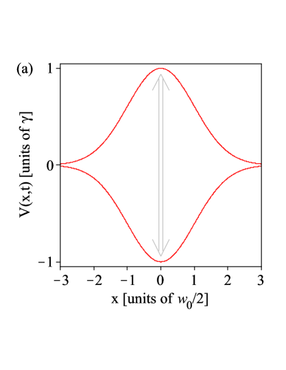
In this section, we consider two simple examples in order to demonstrate the phenomenon found in the preceding section and to compare the derived analytical predictions to results of numerical simulations. The first example to be considered is a particle moving inside an oscillating Gaussian-shaped potential with a vanishing time average of the form

$\displaystyle V^{\textrm{\scriptsize G}}(x,t)=\gamma\exp\left(-\frac{2x^{2}}{w_{0}^{2}}\right)\cos(\omega t+\varphi),$

(15)

which is illustrated in Fig. 1(a).

Potential (15) defines two time scales: The time scale associated with the frequency $\omega$ of the potential’s oscillation and the time scale associated with the oscillation frequency $\omega_{\textrm{\scriptsize osc}}$ of a low energy particle in the minimum instantaneous potential. The theory which was derived in Sec. II is valid for large frequencies $\omega$ compared to the frequencies which are associated with the other time scales of the system. In the following, we therefore consider the regime $\omega\!\gg\!\omega_{\textrm{\scriptsize osc}}$.
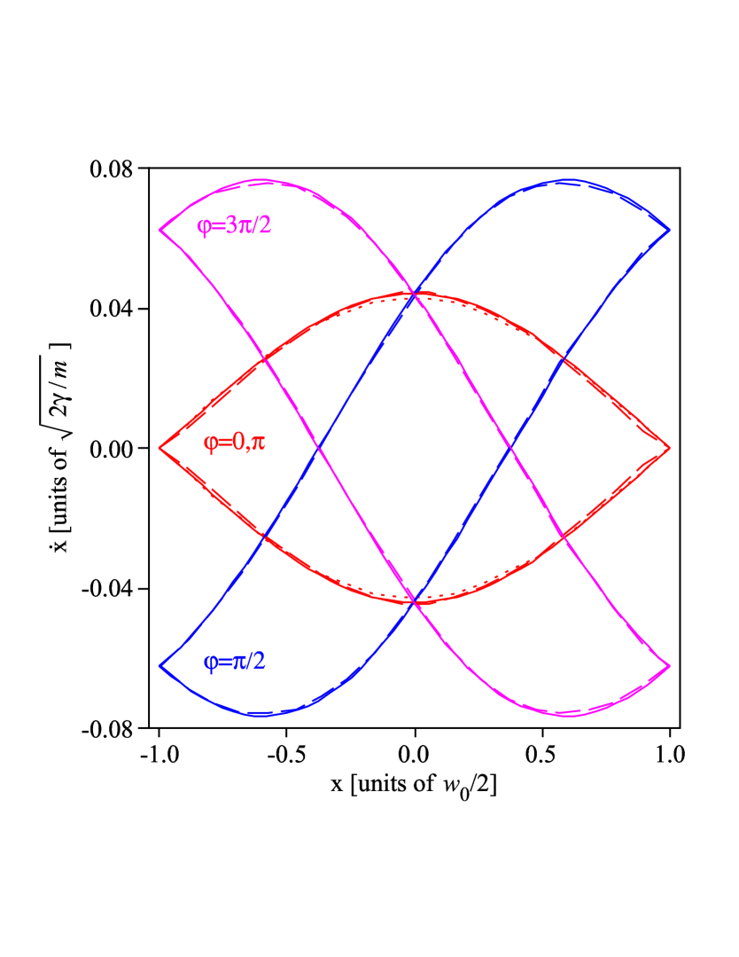
In the preceding section, we showed theoretically, that for correctly chosen initial conditions the position of a trapped particle can be approximated by the position of its slow motion, whereas its velocity cannot be approximated by the velocity of its slow motion. To verify this, we numerically simulate a particle’s trajectory in position and velocity space and compare it to its period-average. This is done by numerically integrating the time dependent Newton equation

$\displaystyle m\ddot{x}=\frac{4\gamma}{w_{0}^{2}}x\exp\left(-\frac{2x^{2}}{w_{0}^{2}}\right)\cos(\omega t+\varphi).$

(16)

The results are shown in Fig. 2.

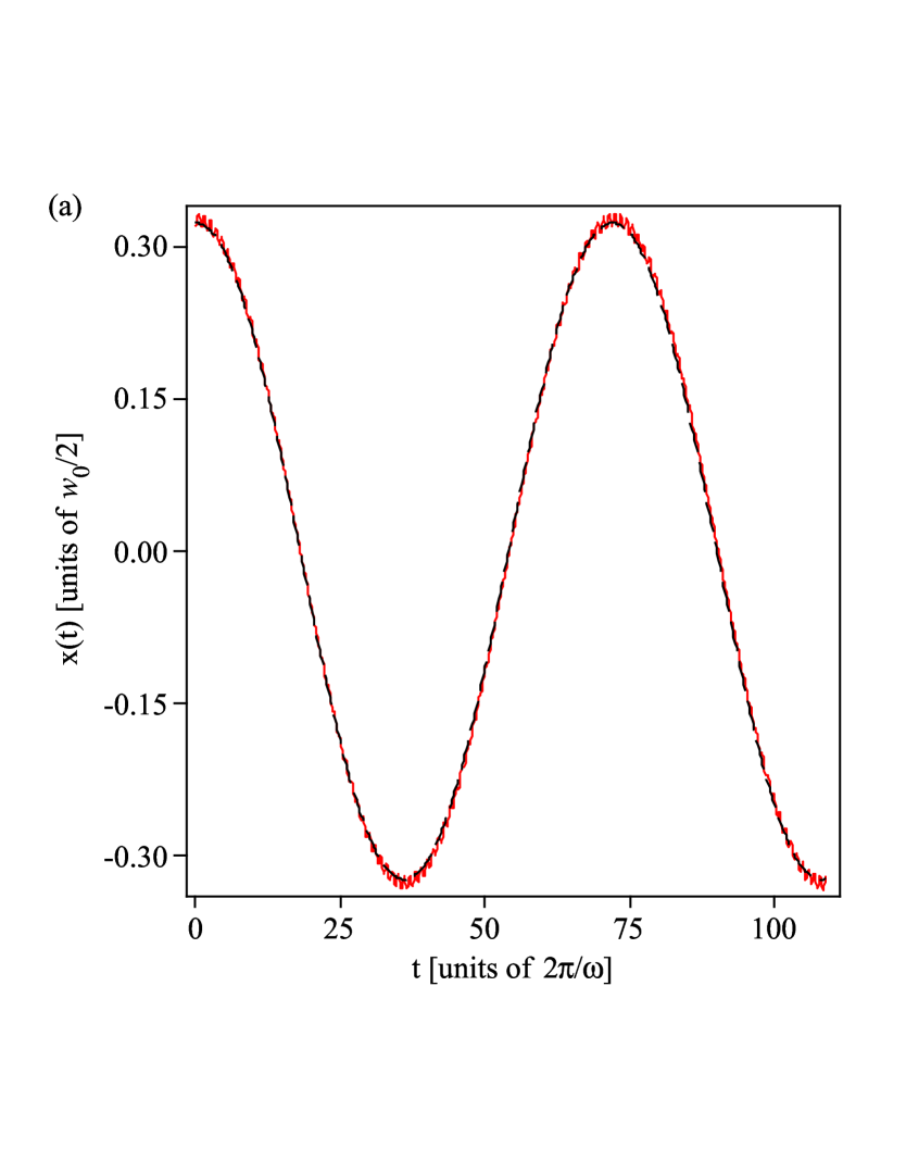
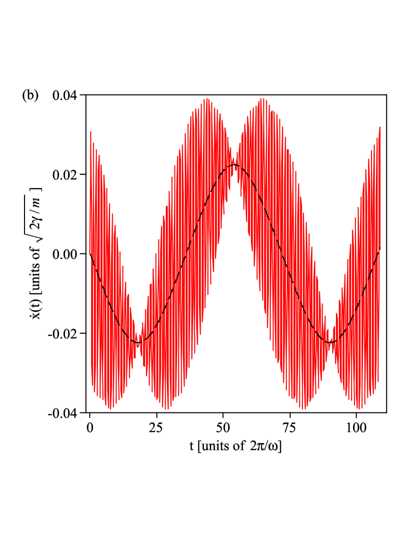
In the figure, one can clearly see that the trajectory in position space is well described by its period-average (Fig. 2(a)), whereas in velocity space (Fig. 2(b)) this is not the case. Additional numerical simulations showed that this result does not change when $\omega$ is increased, in agreement with the derived theory.
In Sec. II, we showed that the significant difference between the particle’s velocity and its period-average (Fig. 2(b)) leads to a dependence of the particle’s motion on the initial phase $\varphi$ of the oscillating potential. To verify this conclusion, we numerically simulate the particle’s trajectory in position space for different $\varphi$ for a given frequency $\omega$ and given initial conditions of the particle. The result is shown in Fig. 3.

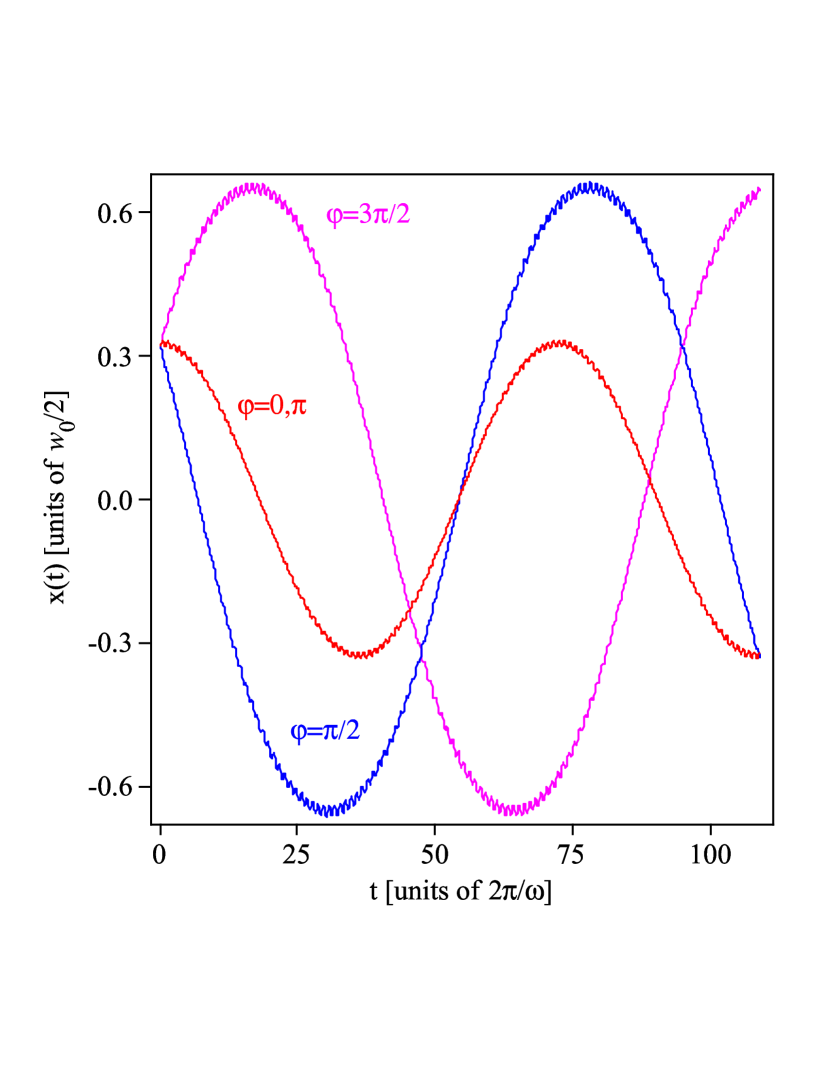
The charted trajectories appreciably differ from each other, as predicted by the derived theory. On the slow time scale they have different phases and different amplitudes. Figure 3 shows as well, that all trajectories appear to be generated from the same time independent effective potential. Since the trajectories for different $\varphi$ are not the same although their initial conditions are, this verifies that the trajectories are determined in addition by a transformation of their initial conditions which depends on $\varphi$. The shown trajectories are almost indistinguishable from their theoretical predictions calculated from equations (5) and (II), which are therefore not shown in the figure.
Another result of Sec. II to be verified by numerical simulations is the prediction of the particle’s motion when phase hops in the oscillating potential’s time modulation function are induced. Figure 4 shows the numerically simulated trajectory of the particle for a phase hop of size $\Delta\varphi\!=\!\mbox{$\frac{\pi}{2}$}$ induced at a time $t=t_{\textrm{\scriptsize ph}}$ for which $\int^{\tau}[\cos(\tau\!+\!\varphi)]_{\tau=\omega t_{\textrm{\tiny ph}}}=0$, $\frac{1}{2}m\dot{X}(t_{\textrm{\scriptsize ph}})^{2}\approx\frac{3}{4}E$, and $\dot{X}(t_{\textrm{\scriptsize ph}})\,V_{1}^{\prime}(X(t_{\textrm{\scriptsize ph}}))>0$.

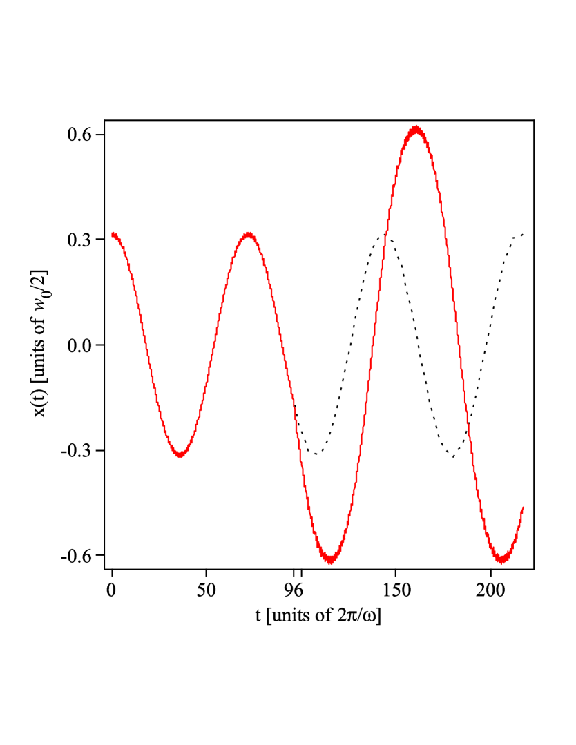
In agreement with the analytical prediction (14), the period-averaged energy of the particle in Fig. 4 indeed changes by a factor of approximately $2.7$. Furthermore, the shown trajectory is almost indistinguishable from its theoretical prediction (not shown in the figure) calculated from equations (5) and (II), whereas the part of the trajectory after the phase hop is obtained from these by assigning the time of the phase hop to the initial time.
Figure 5 shows the numerically simulated trajectory of the particle when several phase hops of the size $\Delta\varphi\!=\!\mbox{$\frac{\pi}{2}$}$ are induced. The moments of the phase hops $t_{i}=t^{(i)}_{\textrm{\scriptsize ph}}$ were chosen such that $\int^{\tau}[\cos(\tau\!+\!\varphi)]_{\tau=\omega t^{(i)}_{\textrm{\tiny ph}}}=0$, $\frac{1}{2}m\dot{X}(t^{(i)}_{\textrm{\scriptsize ph}})^{2}\approx\frac{3}{4}E(t^{(i)}_{\textrm{\scriptsize ph}})$, and $\dot{X}(t^{(i)}_{\textrm{\scriptsize ph}})\,V_{1}^{\prime}(X(t^{(i)}_{\textrm{\scriptsize ph}}))<0$, whereas $X(t^{(i)}_{\textrm{\scriptsize ph}})$, $\dot{X}(t^{(i)}_{\textrm{\scriptsize ph}})$, and $E(t^{(i)}_{\textrm{\scriptsize ph}})$ denote the position, the velocity, and the energy of the particle’s slow motion right before the $i$th phase hop, respectively.

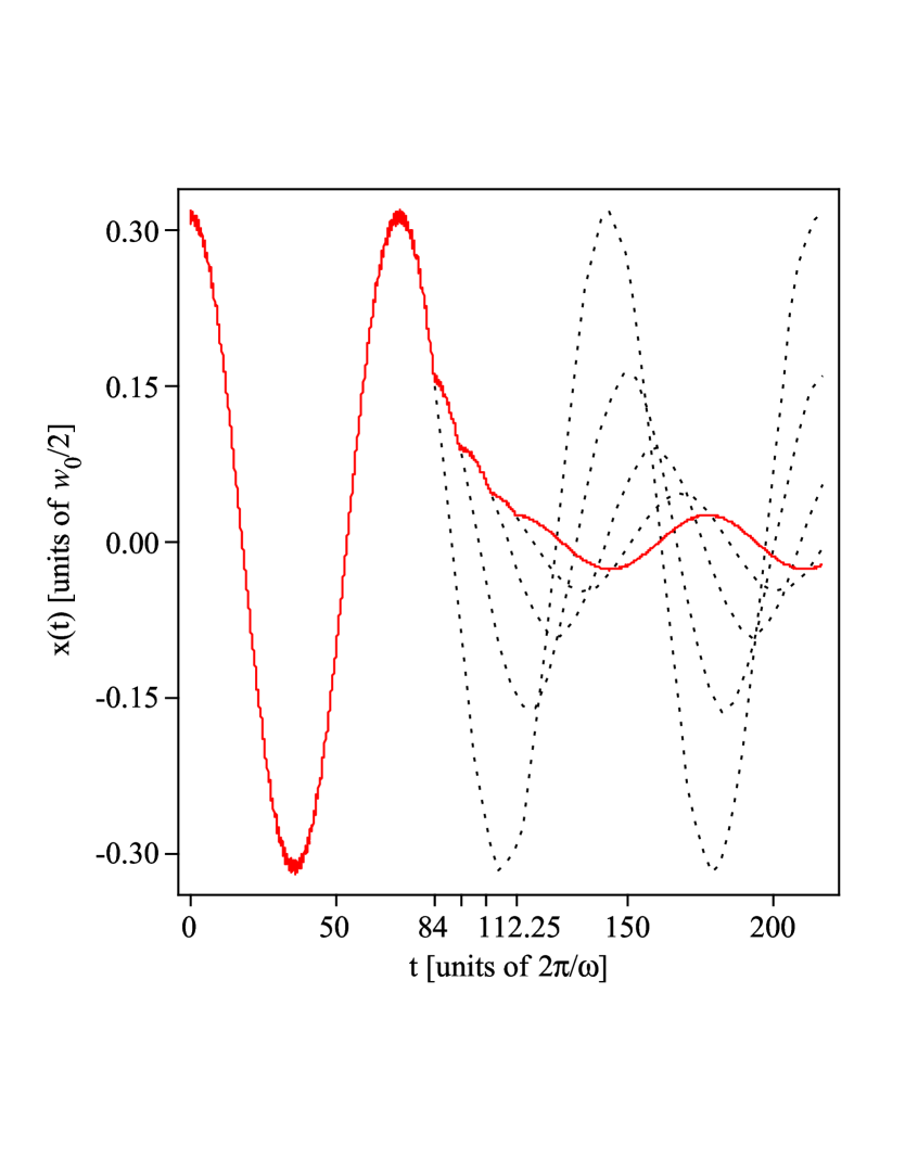
In agreement with the analytical prediction (14), the period-averaged energy of the particle in Fig. 5 changes in total by a factor of approximately $\frac{1}{170}$. Figure 5 demonstrates that this substantial change in energy can be achieved even when the phase hops are induced very quickly one after another (within a fraction of the period of the particle’s slow motion). The shown trajectory is almost indistinguishable from its theoretical prediction (not shown) calculated from Eqs. (5) and (II).
The last theoretical prediction of Sec. II that is to be verified by numerical simulations in the following is the derived equation (10) for the stability region. For the particle inside the oscillating Gaussian-shaped potential (15), it yields

	$\displaystyle\!\!\!\!\!\!\!\!\!\!\dot{x}^{\textrm{\scriptsize(G)}}\!\!$	$\displaystyle\lessgtr$	$\displaystyle\!\!-\frac{1}{m\omega}\frac{4\gamma}{w_{0}^{2}}x\exp\left(\mbox{$-\frac{2x^{2}}{w_{0}^{2}}$}\right)\sin\varphi$		(17)
			$\displaystyle\!\!\pm\frac{1}{m\omega}\frac{\sqrt{8}\gamma}{w_{0}^{2}}\sqrt{\frac{w_{0}^{2}}{4}\exp\left(\mbox{$-1$}\right)-x^{2}\exp\left(\mbox{$-\frac{4x^{2}}{w_{0}^{2}}$}\right)}.$

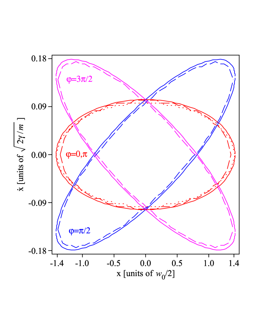
A graph of this analytical prediction of the stability region for different $\varphi$ is shown in Fig. 6 (solid curves). Before comparing it to the results of numerical simulations, we first discuss it separately.

In Fig. 6, one can clearly see that the analytically predicted stability regions for different $\varphi$ significantly differ from each other. For the initial phases $\varphi\!=\!0$ and $\varphi\!=\!\pi$, the stability regions are identical and axially symmetrical to the coordinate axes. For the phases $\varphi\!=\!\mbox{$\frac{\pi}{2}$}$ and $\varphi\!=\!\mbox{$\frac{3\pi}{2}$}$, the stability regions are not axially symmetrical to the coordinate axes and particularly not to the position axis. This demonstrates, that the motion of the particle cannot be determined by a time independent effective potential alone, since the stability region of any time independent potential is due to energy conservation axially symmetric to the position axis. Compared to the stability regions of the phases $\varphi\!=\!0$ and $\varphi\!=\!\pi$, those of the phases $\varphi\!=\!\mbox{$\frac{\pi}{2}$}$ and $\varphi\!=\!\mbox{$\frac{3\pi}{2}$}$ further look distorted and rotated around the origin. One can see, that the area of the stability region is independent of the initial phase $\varphi$, which immediately emerges from equation (10). The overlap of two stability regions of different $\varphi$ in units of their total area, however, depends on the initial phase of the respective overlapping stability regions, but is according to Eq. (10) independent of $\omega$. The spatial width of the stability region is independent of the initial phase $\varphi$ and according to Eq. (10) also independent of $\omega$. Finally, Fig. 6 shows that the boundaries of all stability regions intersect at $x\!=\!0$, and thus the escape velocity of the particle that is initially situated at $x\!=\!0$ is independent of the initial phase $\varphi$, in agreement with the numerical results presented in AbrCha04 . This is, because for $x(0)\!=\!0$ the initial condition transformation (II) is independent of $\varphi$, since it is $V_{1}^{\prime}(0)\!=\!0$.
We now compare the analytical prediction for the stability region (17) to results of numerical simulations, which are shown as dashed and dotted curves in Fig. 6. The numerical simulations were performed as follows: First, the particle’s phase space was discretized into a grid of equally spaced points, each of which define possible initial conditions of the particle. Then, the time dependent Newton equation (16) was integrated numerically for each of these points. Thus, all the points, which generated a trajectory that stayed within a prespecified spatial region within a prespecified large time, were defined as points of the stability region. The prespecified values for the spatial region ($|x|\!\lesssim\!\mbox{$\frac{w_{0}}{2}$}$) and the large time ($t\!\approx\!\mbox{$200\cdot\frac{2\pi}{\omega}$}$) were chosen such that further increase in these values did not change the result appreciably. The step size was chosen to be $\Delta t\!=\!\mbox{$\frac{1}{100}\!\cdot\!\frac{2\pi}{\omega}$}$, since further decrease of the step size did not alter the results appreciably. Figure 6 shows a very good agreement between theory and simulations. Additional simulations showed, that this agreement increases when $\omega$ is increased, as expected from the theory.
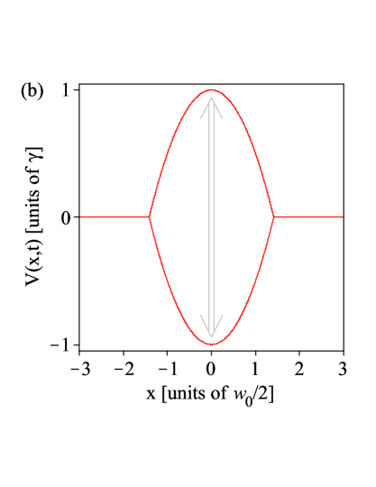
So far we have considered a particle moving inside the oscillating Gaussian-shaped potential (15). Another example to be considered in the following is a particle moving inside an oscillating clipped parabola-shaped potential with a vanishing time average of the form

$\displaystyle V^{\textrm{\scriptsize cp}}(x,t)=V_{1}(x)\cos(\omega t+\varphi),$

(18)

with

$\displaystyle V_{1}(x)=\begin{cases}-kx^{2}+kL^{2}&\mbox{for $|x|\leq L$,}\\ 0&\mbox{else,}\end{cases}$

(19)

which is illustrated in Fig. 1(b). This is a problem able to be solved exactly, because the particle’s time dependent Newton equation

$\displaystyle m\ddot{x}=\begin{cases}2kx\cos(\omega t+\varphi)&\mbox{for $|x|\leq L$,}\\ 0&\mbox{else}\end{cases}$

(20)

is for $|x|\!\leq\!L$ equivalent to the homogeneous Mathieu equation, whose solution is given by a linear combination of the Mathieu functions Pau90 ; LeiBla03 ; MajGhe04 , and for $|x|\!\geq\!L$ it is equivalent to the trivial differential equation $\ddot{x}=0$ of free motion. Therefore, the considered example allows for a comparison between the theory that was derived in Sec. II and the Mathieu theory. We choose $L=\mbox{$\frac{w_{0}}{\sqrt{2}}$}$ and $k=\mbox{$\frac{\gamma}{L^{2}}$}$ so that in Eq. (18) the reference frequency $\omega_{\textrm{\scriptsize osc}}\!=\!\sqrt{\frac{4\gamma}{mw_{0}^{2}}}$ as well as the maximum instantaneous potential depth $\gamma$ are the same as in (15). In the following, we calculate the particle’s stability region – once by using the derived equation (10) and once by applying Mathieu’s theory. Equation (10) yields

$\displaystyle\!\!\dot{x}^{\textrm{\scriptsize(cp)}}\lessgtr-\frac{1}{m\omega}\frac{4\gamma}{w_{0}^{2}}x\sin(\varphi)\pm\frac{1}{m\omega}\frac{2\sqrt{2}\gamma}{w_{0}^{2}}\sqrt{\frac{w_{0}^{2}}{2}-x^{2}}.$

(21)

A graph of this analytical prediction of the stability region is shown in Fig. 7 (solid curves) for different $\varphi$. Figure 7 also shows the results obtained from Mathieu’s theory (dashed and dotted curves).

It can be seen that the stability regions of the particle have the shape of an ellipse. Figure 7 shows a very good agreement of our derived theory and the Mathieu theory. In order to confirm the accuracy of the numerical simulations which we performed for the oscillating Gaussian-shaped potential in the preceding paragraph, we repeated these simulations for the parabola-shaped potential finding that the obtained results were identical to those obtained from Mathieu’s theory. All main results which we demonstrated for the oscillating Gaussian-shaped potential were found also for the oscillating parabola-shaped potential.

In this section, we propose an experiment to verify our theoretical results. Consider an ensemble of atoms that is trapped inside a rapidly oscillating potential with a vanishing time average, whose amplitude is chosen such that the ensemble uniformly fills its stability region. Hence the fraction of atoms which remain trapped after a phase hop of the oscillating potential is induced is equal to the mutual overlap of the stability region with the initial time given by the time right before the phase hop and the stability region with the initial time given by the time right after the phase hop. This overlap is exactly determined by equation (10). It is a function of the time $t_{\textrm{\scriptsize ph}}$ when the phase hop is induced and of the size $\Delta\varphi$ of the phase hop. Figure 8 shows this overlap for a two-dimensional oscillating Gaussian-shaped potential.

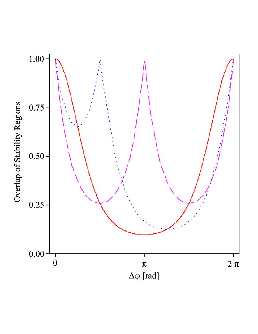
One can see that, regardless of $t_{\textrm{\scriptsize ph}}$, at least $70\%$ of the atoms will leave the trap for appropriate $\Delta\varphi$. Therefore, when measuring the ratio between the numbers of trapped atoms before and after the phase hop for different phase hop sizes, one can expect a clear signal from the experiment.

In conclusion, we investigated the classical dynamics of a particle moving inside a rapidly oscillating potential with a vanishing average. We found, that the motion of such a particle significantly depends on the oscillating potential’s initial phase in the case that the particle is trapped. The effective potential theory described in the literature failed to describe this phenomenon. We found that this theory is incomplete. It states that the motion of the particle is determined by a time independent effective potential, whereas we could show that this is true only if the particle’s initial conditions are transformed according to a non-negligible transformation which is significant even for arbitrarily high frequencies of the potential’s oscillation. We derived this transformation and showed that it depends on the potential’s initial phase which explains the found phenomenon. We also showed that there always exist two initial phases of the oscillating potential such that the transformation can be neglected. Therefore, the effective potential theory in its previous form, which omits this transformation, can only describe these two special cases correctly. The phase dependence offers a new possibility to significantly manipulate the dynamics of a trapped particle. We explicitly calculated the change in a particle’s energy caused by a phase hop in the potential’s modulation function. We found that it is significant for arbitrarily high frequencies of the potential’s oscillation and – in the framework of classical physics – for arbitrarily low energies of the particle. It is the subject of future research to find applications of this novel tool of particle manipulation. The results presented in this article, should also be extended to the quantum regime.

We would like to thank Shmuel Fishman, Roee Ozeri, Nir Bar-Gill, Rami Pugatch and Yoav Sagi for stimulating and inspiring discussions. This research was supported by the “Stiftung der Deutschen Wirtschaft” of the Federal Ministry of Education and Research (BMBF) of Germany and by the MINERVA Foundation.

References

- (1) P.L. Kapitza, Zh. Eksp. Teor. Fiz. 21, 588 (1951).
- (2) L.D. Landau and E.M. Lifschitz, Mechanics (Pergamon Press, Oxford, 1976).
- (3) A.V. Gaponov and M.A. Miller, Zh. Eksp. Teor. Fiz. 34, 242 (1958).
- (4) H.G. Dehmelt, Adv. At. Mol. Phys. 3, 53 (1967).
- (5) I.C. Percival and D. Richards, Introduction to Dynamics (Cambridge University Press, London, 1982).
- (6) B.B. Nadezhdin and E.A. Oks, Pis’ma Zh. Tekh. Fiz. 12, 1237 (1986).
- (7) M. Combescure, Ann. Inst. Henri Poincare A 44, 293 (1986).
- (8) R.J. Cook, D.G. Shankland and A.L. Wells, Phys. Rev. A 31, 564 (1985).
- (9) T.P. Grozdanov and M.J. Raković, Phys. Rev. A 38, 1739 (1988).
- (10) S. Rahav, I. Gilary and S. Fishman, Phys. Rev. Lett. 91, 110404 (2003); Phys. Rev. A 68, 013820 (2003).
- (11) W. Paul, Rev. Mod. Phys. 62, 531 (1990).
- (12) R. Blatt, P. Gill and R.C. Thompson, J. Mod. Opt. 32, 193 (1992).
- (13) J.I. Cirac and P. Zoller, Phys. Rev. Lett. 74, 4091 (1995).
- (14) D. Leibfried, R. Blatt, C. Monroe and D. Wineland, Rev. Mod. Phys. 75, 281 (2003).
- (15) F.G. Major, V.N. Gheorghe and G. Werth, Charged Particle Traps: Physics and Techniques of Charged Particle Field Confinement (Springer-Verlag, New York, 2004).
- (16) U. Geigenmüller, U.M. Titulaer and B.U. Felderhof, Physica A 119, 41 (1983).
- (17) F. Haake and M. Lewenstein, Phys. Rev. A 28, 3606 (1983).
- (18) S.M. Cox and A.J. Roberts, Physica D 85, 126 (1995).
- (19) N. Friedman, A. Kaplan, D. Carasso and N. Davidson, Phys. Rev. Lett. 86, 1518 (2001).
- (20) J.A. Sanders and F. Verhulst, Averaging Methods in Nonlinear Dynamical Systems (Springer-Verlag, New York, 1985).
- (21) G.T. Abraham, A. Chatterjee and A.G. Menon, Int. J. Mass Spectrom. 231, 1 (2004).