Partitioning of a polymer chain between a confining cavity and a gel

The problem of partitioning of a polymer chain confined to move within large cavities embedded into a hydrogel has received attention with some interesting experiments performed by Liu et al. [1]. These authors investigated the so called “entropic trapping” phenomenon, which describes the preferential localization of a polymer chain within large cavities embedded in a hydrogel due to the larger conformational entropy of the chain in them. Therefore, this phenomenon has been suggested as a basis for potential new methods of polymer separation. In this context, the problem is also relevant and can lead to better understanding and possible improvement of many existing separation methods, such as membrane separation, filtration, gel electrophoresis, size exclusion chromatography, etc. [2], all of which utilize the dependence of macromolecular mobility through a network of random obstacles on molecular properties, such as molecular weight, monomer charge, electrolyte composition, etc. The practical importance of these techniques has motivated a number of investigations of polymer separation between cavities of different size [3–7].

In our earlier work [6, 7] we used lattice field theory calculations to study polymer separation between two spheres of different size—a simplified model of the more complicated system of the polymer moving between large cavities embedded in a hydrogel, with the larger sphere playing the role of the cavities and the small sphere corresponding to the connecting channels in the gel. We investigated the dependence of the partition coefficient $K$, defined as the ratio of the average number of monomers in the two respective spheres, as a function of the total number of monomers in the chain, the excluded volume interaction between them, the monomer charge, and the concentration of electrolytes in the solution. Our results were qualitatively in accord with the experiments of Liu et al. [1] and with related computer simulations [8].

In this work we apply the lattice field theory approach to the more complex system of a polymer chain moving within a large spherical cavity embedded in a network of random obstacles.

In Section 2 of the paper, for continuity of the presentation, we review the lattice field theory of charged polymer chains in electrolyte solution [7]. In Section 3 we describe the Lanczos approach for finding the energy spectrum of the Schrödinger Hamiltonian problem (arising from the polymer part of the partition function [7]), and the resolvent approach for extracting the corresponding eigenvectors. Section 4 describes the numerical procedure for solving the mean field equations of the system, and in Section 5 we present and discuss our results. In Section 6 we conclude our presentation.

In Ref. [9] we derived the following functional integral expression for the full partition function of a charged polymer in an electrolyte solution with short-range monomer repulsion interactions

$$Z=\int D\chi(\vec{r})D\omega(\vec{r})e^{\frac{\beta\varepsilon}{8\pi}\int\chi\Delta\chi d\vec{r}-\frac{\lambda}{2}\int\omega(\vec{r})^{2}d\vec{r}+c_{+}\int e^{ie\beta\chi}d\vec{r}+c_{-}\int e^{-ie\beta\chi}d\vec{r}}Z_{Schr}(\chi,\omega)\,.$$

(1)

Here, $\beta{=}1/kT$ is the inverse temperature, $\varepsilon$ is the dielectric constant of the solution, $e$ is the proton charge, $\lambda$ is a measure of the strength of the excluded volume interaction, $\chi$ and $\omega$ are auxiliary fields, $c_{\pm}{=}e^{\beta\mu_{\pm}}/\lambda_{\pm}^{3}$ with $\mu_{\pm}$ and $\lambda_{\pm}$ being the chemical potentials and the thermal deBroglie wavelengths for the ions, respectively. The polymer part $Z_{Schr}(\chi,\omega)$ in (1) refers to a Euclidean-time ($T{=}M{=}$total number of monomers) amplitude for an equivalent Schrödinger problem based on the Hamiltonian

$$H\equiv-\frac{a_{p}^{2}}{6}\vec{\nabla}^{2}+\lambda\omega_{c}(\vec{r})+\beta pe\chi_{c}(\vec{r})\,,$$

(2)

where $a_{p}$ is the Kuhn length and $p$ is the charge per monomer. The mean-field equations corresponding to the purely-real saddle-point configuration fields $\chi_{c}=i\chi$, $\omega_{c}=i\omega$ are obtained by setting the variational derivative of the exponent in the full functional integral (1) to zero. For the case of a polymer with free ends (the only situation considered in this paper), the polymer amplitude $Z_{\rm Schr}$ can be written in terms of sums over eigenstates of $H$ as follows [7]:

	$\displaystyle Z_{Schr}$	$\displaystyle=$	$\displaystyle{\int}dx_{i}dx_{f}\sum_{n}\Psi_{n}(x_{i})\Psi_{n}(x_{f})e^{-ME_{n}}$		(3)
		$\displaystyle=$	$\displaystyle\sum_{n}A_{n}^{2}e^{-ME_{n}}\,{\equiv}\,e^{F_{pol}}\,,$

where $E_{n}$ is the $n$-th energy eigenvalue,

$$A_{n}\equiv{\int}d\vec{r}\,\Psi_{n}(\vec{r})\,,$$

(4)

and

$$F_{pol}=\ln\left(\sum_{n}A_{n}^{2}e^{-ME_{n}}\right)\,$$

(5)

is the negative of the polymer contribution to the free energy. Thus, the mean-field result for the negative of the total free energy is

$$F=\int d\vec{r}\left\{\frac{\beta\varepsilon}{8\pi}\left|\vec{\nabla}\chi_{c}\right|^{2}+\frac{\lambda}{2}\omega_{c}^{2}+c_{+}e^{\beta e\chi_{c}}+c_{-}e^{-\beta e\chi_{c}}\right\}+F_{pol}(\chi_{c},\omega_{c})\,.$$

(6)

Varying the functional (6) with respect to the fields $\chi_{c},\omega_{c}$ one obtains the mean-field equations

	$\displaystyle\frac{\varepsilon}{4\pi e}\vec{\nabla}^{2}\chi_{c}(\vec{r})$	$\displaystyle=$	$\displaystyle c_{+}e^{\beta e\chi_{c}(\vec{r})}-c_{-}e^{-\beta e\chi_{c}(\vec{r})}-p\rho(\vec{r})\,,$		(7)
	$\displaystyle\frac{a_{p}^{2}}{6}\vec{\nabla}^{2}\Psi_{n}(\vec{r})$	$\displaystyle=$	$\displaystyle\lambda\rho(\vec{r})\Psi_{n}(\vec{r})+\beta pe\chi_{c}(\vec{r})\Psi_{n}(\vec{r})-(E_{n}-V_{m}(\vec{r}))\Psi_{n}(\vec{r})\,,$		(8)

where $\rho$, defined as

$$\rho(\vec{r}){\equiv}-\frac{\sum_{n,m}\frac{A_{n}\Psi_{n}A_{m}\Psi_{m}}{E_{n}-E_{m}}\left(e^{-ME_{n}}-e^{-ME_{m}}\right)}{\sum_{n}A_{n}^{2}e^{-ME_{n}}}\,,$$

(9)

is the total monomer density. The equations presented here apply for polymer chains of arbitrary length, provided all (or a sufficient number) of states are included in the sums above. The single-particle potential $V_{m}(\vec{r})$ has been included to enforce an exclusion region for the monomers [9]. Note that the parameters $c_{\pm}$ are exponentials of the chemical potentials $\mu_{\pm}$ for positively and negatively charged ions. The numbers of these ions must be fixed by suitably adjusting $c_{\pm}$ to satisfy the relations

$$n_{\pm}=c_{\pm}\frac{\partial\log{(Z)}}{\partial c_{\pm}}=c_{\pm}\int e^{\pm\beta e\chi_{c}}d\vec{r}\,.$$

(10)

The advantage of working with $F$ is that, as shown in Ref. [7], it has a unique minimum, and thus, can be used to guide a numerical search for the mean electrostatic and monomer density fields. Once the mean fields have been computed, the defining relation ${\ln}Z{\cong}F(\chi_{c},\omega_{c})$ can be used to obtain free energies of various types. For example, the Helmholtz free energy $A$ (corresponding to fixed numbers of monomers and impurity ions) is given by

$$\beta A=n_{+}\ln c_{+}+n_{-}\ln c_{-}-F(\chi_{c},\omega_{c})\,.$$

(11)

Following the procedure of Ref. [9], we now move from the continuum to a discrete 3-dimensional lattice by rescaling according to

	$\displaystyle f(\vec{r})$	$\displaystyle{\rightarrow}$	$\displaystyle{\beta}e\chi_{c}(\vec{r})$
	$\displaystyle\Psi_{N}(\vec{r})$	$\displaystyle{\rightarrow}$	$\displaystyle a_{l}^{3/2}\Psi_{N}(\vec{r})$

and multiplying Eq. (7) by $a_{l}^{3}$ ($a_{l}$ being the lattice spacing). This leads to the following discretized version of equations (7) and (8) on a 3D lattice:

	$\displaystyle\alpha\sum_{\vec{m}}\Delta_{\vec{n}\vec{m}}f_{\vec{m}}$	$\displaystyle=$	$\displaystyle\gamma_{+}e^{f_{\vec{n}}}-\gamma_{-}e^{-f_{\vec{n}}}-p\rho_{\vec{n}}\,,$		(12)
	$\displaystyle\frac{a_{p}^{2}}{6a_{l}^{2}}\sum_{\vec{m}}\Delta_{\vec{n}\vec{m}}\Psi_{N,\vec{m}}$	$\displaystyle=$	$\displaystyle\frac{{\lambda}M}{a_{l}^{3}}\rho_{\vec{n}}\Psi_{N,\vec{n}}+pf_{\vec{n}}\Psi_{N,\vec{n}}-E_{N}\Psi_{N,\vec{n}}\,,$		(13)

where

	$\displaystyle\alpha$	$\displaystyle=$	$\displaystyle\frac{{\varepsilon}a_{l}}{4\pi{\beta}e^{2}}\,,$		(14)
	$\displaystyle\gamma_{\pm}$	$\displaystyle=$	$\displaystyle\frac{n_{\pm}}{\sum_{\vec{n}}e^{\pm f_{\vec{n}}}}\,,$		(15)

and the wavefunctions are dimensionless and normalized according to

$$\sum_{\vec{n}}\Psi_{N,\vec{n}}^{2}=1\;;\;$$

(16)

thus, the density $\rho_{\vec{n}}$ sums to the total number of monomers, $M$.

The simultaneous relaxation solution of Equations (12) and (13) requires a rapid and efficient extraction of the eigenvalues and low-lying eigenvectors of the operator $H$, which amounts—once the problem has been set up on a discrete finite 3-dimensional lattice—to a large sparse real symmetric matrix.

We have found it convenient to use distinct algorithms to extract the low-lying spectrum and eigenvectors of $H$ (typically we need on the order of 10–30 of the lowest states for the shortest polymer chains studied here, while for the longest polymer chains only one to three states suffice). The eigenvalues are extracted using the Lanczos technique [10]. Starting from a random initial vector $w_{0}\equiv v_{1}$, one generates a series of orthonormal vectors $v_{1},v_{2},...$ by the following recursion:

	$\displaystyle v_{n+1}$	$\displaystyle=$	$\displaystyle w_{n}/\beta_{n}\,,$
	$\displaystyle n$	$\displaystyle\rightarrow$	$\displaystyle n+1\,,$
	$\displaystyle\alpha_{n}$	$\displaystyle=$	$\displaystyle(v_{n},Hv_{n})\,,$
	$\displaystyle w_{n}$	$\displaystyle=$	$\displaystyle(H-\alpha_{n}I)v_{n}-\beta_{n-1}v_{n-1}\,,$
	$\displaystyle\beta_{n}$	$\displaystyle=$	$\displaystyle\sqrt{(w_{n},w_{n})}\,,$

where $\alpha_{n},\beta_{n}$ are real numbers, with $\beta_{0}=1$ and $v_{0}=0$. The matrix of $H$ in the basis spanned by $v_{n}$ is tridiagonal with the number $\alpha_{n}$ ($\beta_{n}$) on the diagonal (respectively, super/sub diagonal). Carrying the Lanczos recursion to order $N$, diagonalization of the resulting $N{\times}N$ tridiagonal matrix leads, for large $N$, to increasingly accurate approximants to the exact eigenvalues of $H$. The presence of spurious eigenvalues (which must be removed by the sieve method of Cullum and Willoughby [11]) means that typically a few hundred Lanczos steps must be performed to extract the lowest 30 or 40 eigenvalues of $H$ (for dimensions of $H$ of order 10⁵ as studied here) to double precision.

Once the low-lying spectrum of $H$ has been extracted by the Lanczos procedure, as outlined above, the corresponding eigenvectors are best obtained by a resolvent procedure. Supposing $\lambda_{n}$ to be the exact $n$th eigenvalue of $H$ (as obtained by the Lanczos method), and $\psi_{n}$ the corresponding eigenvector, then for any random vector $\psi_{\rm ran}$ with nonzero overlap with $\psi_{n}$, the vector obtained by applying the resolvent

$$\psi_{n,\rm approx}\equiv\frac{1}{\lambda_{n}+\epsilon-H}\psi_{\rm ran}$$

(17)

is an increasingly accurate (unnormalized) approximant to the exact eigenvector $\psi_{n}$ as the shift $\epsilon$ is taken to zero. A convenient algorithm for performing the desired inverse is the biconjugate gradient method (see routine linbcg in [12]). We have found the combination of Lanczos and conjugate gradient techniques to be a rapid and efficient approach to the extraction of the needed low-lying spectrum.

Equations (12) and (13) are solved simultaneously using the following relaxation procedure [9]. First, the Schrödinger Eq. (13) is solved for $f_{\vec{n}}{=}0$ and ignoring the nonlinear (monomer repulsion) potential term. The resulting $\Psi_{N,\vec{n}}$’s and corresponding energy levels $E_{N}$ (wavefunctions and energy eigenvalues of a particle confined to the cavity in a gel system) are used to calculate $\rho_{\vec{n}}$, then the Poisson-Boltzmann Eq. (12) is solved at each lattice point using a simple line minimization procedure [13]. The process is repeated and the coefficients $\gamma_{\pm}$ are updated after a few iterations until a predetermined accuracy is achieved. Then the resulting $f_{\vec{n}}$ is used in Eq. (13), which is solved using the Lanczos method [10] for a new set of $\Psi_{N,\vec{n}}$’s to be used in calculating an updated version of the monomer density $\rho_{\vec{n}}$. This density is then inserted into Eq. (12) and a new version of $f_{\vec{n}}$ is computed. For numerical stability, the updated $f_{\vec{n}}$ inserted into Eq. (13) is obtained by adding a small fraction of the new $f_{\vec{n}}$ (just obtained from Eq. (12)) to the old one (saved from the previous iteration). The same “slow charging” procedure is used for updating $\rho_{\vec{n}}$ in the nonlinear potential term of the Schrödinger equation (13).

This numerical procedure has been applied to the system of a polymer chain moving within a cavity embedded in a network of random obstacles. We carve a spherical cavity of radius $10a_{l}$ in the middle a cube with a side-length of $40a_{l}$ on $40^{3}$ lattice. The Kuhn length, $a_{p}=2a_{l}$, and in absolute units $a_{p}=5$Å. Then the random obstacles are created by randomly selecting 20% of the remaining lattice points in the cube outside the carved sphere to be off limits for the polymer chain. Thus, the random obstacles take 20% of the gel, that is, 80% of the gel volume plus the cavity volume is available for the chain to move in. On the other hand, the impurity ions are free to move within the whole volume of the system. The monomer repulsion parameter $\lambda$ is fixed throughout the computations through the dimensionless parameter $\zeta$ by the following relation:

$$\zeta=4\pi\frac{\lambda}{a_{p}^{3}}\,,$$

(18)

and the dimensionless parameter $\zeta=5$.

We have computed the log of the partition coefficient $K\equiv\left<M_{1}\right>/\left<M_{2}\right>$, where $\left<M_{1}\right>$ and $\left<M_{2}\right>$ are the number of monomers in the spherical cavity and the remaining gel, respectively, as a function of the total number of monomers in the system, $M=\left<M_{1}\right>+\left<M_{2}\right>$, for varying monomer charge $p$ and varying number of ions in the system. In Fig. 1 we show the plot of $\ln{K}$ vs $M$ for two different monomer charges, $p=-0.1$ and $p=-0.2$ (all in units of $e$), and a fixed number of 600 negative impurity coions in the system, while the number of the positive counterions is fixed according to the condition for electroneutrality.

We see that the partition coefficient $K$ increases with $M$ for only the shortest polymer chains, goes through a turnover, and from then on decreases continuously as the number of monomers is increased. As in our previous work [6, 7], we observe that smaller monomer charge leads to higher partition coefficient, due to the weaker repulsion between the monomers. In Fig. 2 we show how the partition coefficient varies as we vary the number of negative impurity ions in the system. As expected, the higher number of ions leads to better screening of the monomer charges, hence less repulsion and larger $K$.

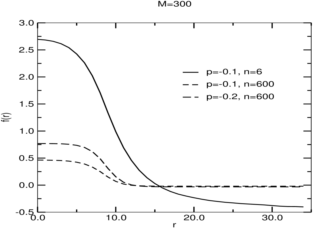
Qualitatively, this behavior is similar to what we observed in our previous work [6, 7]; however, the partition coefficient shown here decreases for almost the whole range of $M$, and is, in fact, much larger than the coefficients reported earlier [6, 7] for partitioning of a polymer chain between two spheres. This can be explained as a result of the much smaller voids that arise between the random obstacles in the gel outside of the spherical cavity, compared to the smaller of the two spheres treated in [6, 7], which, in the Schrödinger language, means that, even though the volume available for the polymer chain outside of the spherical cavity is much greater than the volume of the cavity itself, the energy levels of the excited states which lead to a higher monomer density outside of the cavity are too high (due to the strong confinement in the narrow voids), so that the chain is largely confined to the cavity. Only for the cases of very large $M$ do we observe a non-negligible monomer density outside of the cavity. This is illustrated in Figs. 3 and 4, where we plot the averaged radial density of monomers starting from the center of the spherical cavity for the three different sets of monomer charge and impurity ion concentration parameters presented here. In Fig. 3 we plot the radial density for the case of relatively small number of monomers, $M=40$, and we see that virtually all of the monomers are confined to the spherical cavity, while in Fig. 4, which represents the case of $M=300$, we observe a small but non-negligible contribution to the monomer density from the region outside of the cavity.

In Figs. 5 and 6 we show the plots of the electric potential $f(r)$ corresponding to the parameters of Figs. 3 and 4, respectively. We can qualitatively compare the results from Figs. 3–6 to our previous results in [9], where we computed the monomer density and the electric potential for a charged polymer chain confined to move within a sphere. It is clear that in both cases the shape of the monomer density distribution and the electric potential are quite similar, which is an illustration of the fact that the spherical cavity embedded in the gel does indeed act as an “entropic trap” for the polymer chain, and for most of the range of reasonable physical parameters the system behaves approximately as a polymer chain in a spherical cavity. In Figs. 5 and 6 we see that, for the case of lower counterion numbers, the potential $f(r)$ drops to negative values at large radial distance. Nevertheless, it does approach (up to finite lattice size corrections) zero slope, or equivalently, zero electric field, consistent with the overall electrical neutrality of the system.

We have applied a previously developed lattice field theory approach to the statistical mechanics of a charged polymer chain in electrolyte solution [9, 6, 7] to the problem of a charged polymer chain moving in a spherical cavity embedded in a gel. This problem is more relevant to real experimental situations involving charged polymer chains in a complex environment than the two-sphere problem studied by us earlier [6, 7]. The results of this work demonstrate the capability of the approach to treat more complex systems of arbitrary shape in three dimensions, and also confirm the expectations that a large spherical void carved out from a network of random obstacles can act as a “trap” for polymer chains, and therefore, may serve as a prototype for new methods of polymer separation based on macromolecular weight, monomer charge, and/or electrolyte composition. The results presented here confirm our previous contention [9, 6, 7] that chains with smaller monomer charge would be easier to separate by a technique exploiting the idea of “entropic trapping.” Similarly, for chains with fixed monomer charge, a better separation would be achieved in solutions with higher impurity ion concentration—a parameter which is typically varied in the laboratory.

It is important to note that the method used here is based on the mean field approximation, and therefore, the results should be considered only as qualitative. Nevertheless, one can expect that the long range of the electrostatic interaction and the strong confinement of the polymer chain inside the spherical cavity would result in weakly fluctuating density and electrostatic fields and would make the mean field approximation reliable [14].

Acknowledgments: R.D.C. gratefully acknowledges the support of NSF grant CHE-0518044. The research of A. Duncan is supported in part by NSF contract PHY-0554660.

References

- [1] L. Liu, P. Li and S.A. Asher, Nature 397, 141 (1999); L. Liu, P. Li and S.A. Asher, J. Am. Chem. Soc. 121, 4040 (1999).
- [2] D. Rodbard and A. Chrambach, Proc. Nat. Acad. Sci. USA 65, 970 (1970); G. Guillot, L. Leger and F. Rondelez, Macromolecules 18, 2531 (1985).
- [3] E.F. Casassa, Polymer Lett. 5, 773 (1967).
- [4] E.F. Casassa and Y. Tagami, Macromolecules 2, 14 (1967).
- [5] M. Muthukumar and A. Baumgärtner, Macromolecules 22, 1937 (1989).
- [6] S. Tsonchev and R.D. Coalson, Chem. Phys. Lett. 327, 238 (2000).
- [7] S. Tsonchev, R.D. Coalson, and A. Duncan, Phys. Rev. E 62, 799 (2000).
- [8] S.-S. Chern and R.D. Coalson, J. Chem. Phys. 111, 1778 (1999).
- [9] S. Tsonchev, R.D. Coalson and A. Duncan, Phys. Rev. E. 60, 4257 (1999).
- [10] G. H. Golub and C. F. Van Loan, Matrix Computations (Johns Hopkins University Press, Baltimore, 1996).
- [11] J. Cullum and R.A. Willoughby, J. Comput. Phys. 44, 329 (1981).
- [12] W.H. Press, B.P. Flannery, S.A. Teukolsky, and W.T. Vetterling, Numerical Recipes in C: The Art of Scientific Computing (Cambridge University Press, Cambridge, 1992).
- [13] A. M. Walsh and R. D. Coalson, J. Chem. Phys. 100, 1559 (1994).
- [14] S. Tsonchev, R.D. Coalson, S.-S. Chern, and A. Duncan, J. Chem. Phys. 113, 8381 (2000).