Dorian S. Abbot \extraaffilDepartment of the Geophysical Sciences, University of Chicago \extraauthorJonathan Weare \extraaffilCourant Institute of Mathematical Sciences, New York University
Path properties of atmospheric transitions: illustration with a low-order sudden stratospheric warming model
Abstract
Many rare weather events, including hurricanes, droughts, and floods, dramatically impact human life. To accurately forecast these events and characterize their climatology requires specialized mathematical techniques to fully leverage the limited data that are available. Here we describe transition path theory (TPT), a framework originally developed for molecular simulation, and argue that it is a useful paradigm for developing mechanistic understanding of rare climate events. TPT provides a method to calculate statistical properties of the paths into the event. As an initial demonstration of the utility of TPT, we analyze a low-order model of sudden stratospheric warming (SSW), a dramatic disturbance to the polar vortex which can induce extreme cold spells at the surface in the midlatitudes. SSW events pose a major challenge for seasonal weather prediction because of their rapid, complex onset and development. Climate models struggle to capture the long-term statistics of SSW, owing to their diversity and intermittent nature. We use a stochastically forced Holton-Mass-type model with two stable states, corresponding to radiative equilibrium and a vacillating SSW-like regime. In this stochastic bistable setting, from certain probabilistic forecasts TPT facilitates estimation of dominant transition pathways and return times of transitions. These “dynamical statistics” are obtained by solving partial differential equations in the model’s phase space. With future application to more complex models, TPT and its constituent quantities promise to improve the predictability of extreme weather events, through both generation and principled evaluation of forecasts.
1 Introduction and background
The polar winter stratosphere typically supports a strong, cyclonic polar vortex, maintained by the thermal wind relation and meridional temperature gradient. A sudden stratospheric warming (SSW) event is a large excursion from this normal state, which can take many different forms. In split-type SSWs, the vortex splits completely in two. In displacement-type SSWs the vortex displaces far away from the pole (these can be considered wavenumber-2 and wavenumber-1 disturbances, respectively). Both types are “major” warmings, as the mean zonal wind reverses. In a “minor” warming, the zonal wind slows down significantly without completely reversing (Butler et al., 2015).
SSW is a rare event occurring about twice every three years, depending on the definition used (Butler et al., 2015). Its effects can propagate downward into the troposphere, altering the tropospheric jetstream and inducing extreme midlatitude surface weather events, including cold spells and precipitation (Baldwin and Dunkerton, 2001; Thompson et al., 2002). Abrupt cold spells severely stress infrastructures, economies and human lives, and every bit of extra prediction lead time is helpful for adaptation. Unfortunately, numerical weather prediction struggles to forecast SSW at any lead time longer than about two weeks (Tripathi et al., 2016). Understanding SSW is therefore important for practical forecasting as well as science, but this task remains difficult. Several different geophysical fields are often used as indices of SSW onset. One simple indicator is zonal-mean zonal wind at N, which defines thresholds for minor and major warming (Charlton and Polvani, 2007; Butler et al., 2015). Another common indicator is the 10hPa geopotential height field, which was used by Inatsu et al. (2015) to estimate a fluctuation-dissipation relation in its leading empirical orthogonal functions (EOFs). Many studies have examined SSW precursors and dominant pathways through simulation and observation. Limpasuvan et al. (2004), for instance, catalogued the various wavenumber forcings, heat fluxes and zonal wind anomalies that accompanied each stage of SSW events from reanalysis data. While planetary wave forcing from the troposphere is an accepted proximal cause of SSW, the polar vortex’s susceptibility to such forcing, or “preconditioning”, is a nontrivial and debated function of its geometry (Albers and Birner, 2014; Bancalá et al., 2012). Tropospheric blocking is also thought to be linked to SSW; Martius et al. (2009) and Bao et al. (2017) found blocking to precede many major SSW events of the past half century. The diversity and complex life cycle of SSWs makes it difficult to build a unified picture of their onset.
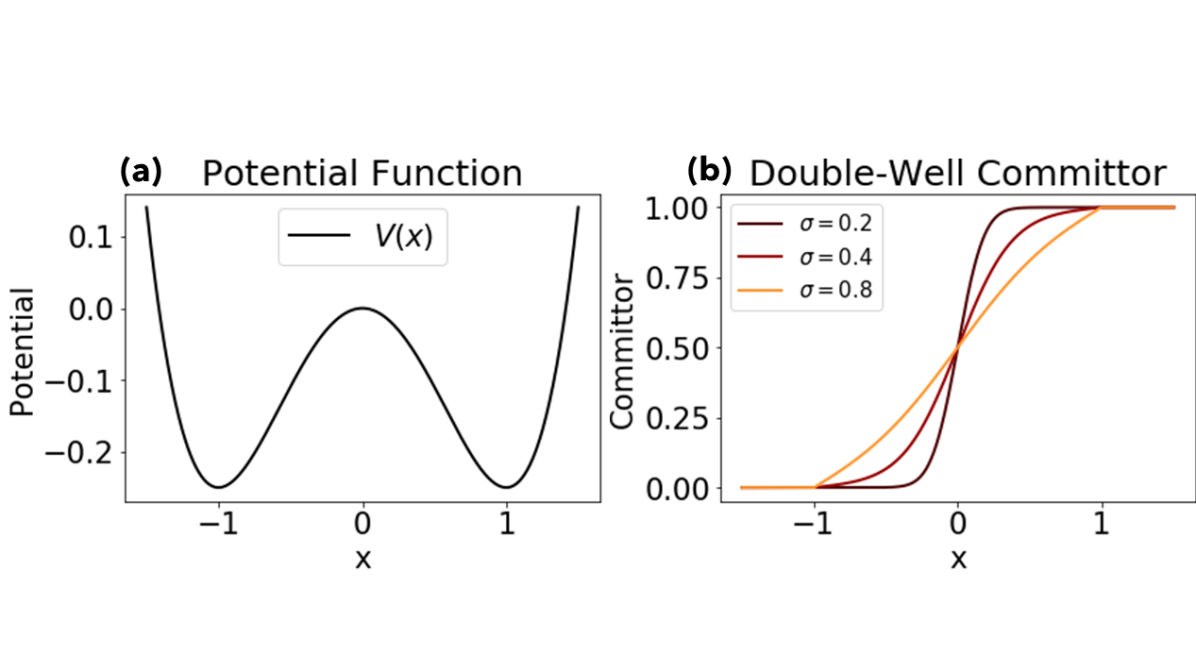
In this article, we are interested in developing a detailed understanding of transition events between two states, at least one of which is typically long-lived. Consider, for example, a particle with position moving in the double well potential energy landscape (illustrated in Figure 1) and forced by stochastic white noise : . If the system starts in the left well, it will tend to remain there a while, but occasionally the stochastic forcing will push it over the barrier into the right well. The natural predictor for this event is the committor: the probability of reaching the right well before the left well.
We denote this function by , which solves the Kolmogorov backward equation (to be introduced later). For this simple system the equation takes a form which can be solved exactly:
| (1) | |||
| (2) |
Note that the boundary conditions are implied by the probabilistic interpratation.
The committor is plotted in the right panel of Figure 1 for various noise levels. N.B., the potential landscape picture is not fully general, but is a useful mental model. The equations that determine will be presented in section 2.
In the case of SSW, the long-lived states are the steady and disturbed circulation regimes of the stratospheric polar vortex. Recent work by Yasuda et al. (2017) has studied SSW in an equilibrium statistical mechanics framework, with these two stable states as saddle points of energy functionals. TPT takes a complementary non-equilibrium view, describing the long-time (steady-state) statistics of trajectories between the two states. For example, TPT introduces a probability density of reactive trajectories (or “reactive density”) indicating the regions where trajectories tend to spend their time en route from A to B. The system is said to be reactive at a point in time if it has most recently visited and will next visit . The associated probability current of reactive trajectories (or “reactive current”) indicates the preferred direction and speed of transition paths. These detailed descriptors of the mechanism underlying a rare event can be expressed in terms of probabilistic forecasts like the committor , the probability of entering state A before reaching state B from a given initial condition (not in either A or B). The committor is the ideal probabilistic forecast in the usual variance-minimizing sense of conditional expectations (Durrett, 2013). Any other predictor of a transition derived through experiments and observations, such as vortex preconditioning and forcing at different wavenumbers (Albers and Birner, 2014; Bancalá et al., 2012; Martius et al., 2009; Bao et al., 2017) necessarily corresponds to an approximation of the committor.
Ensemble simulation is a commonly used method to estimate the committor at a single given initial condition by measuring the fraction of ensemble trajectories that achieve the rare event. This is challenging because many simulations are needed to generate enough rare events for significant statistical power. Recent and ongoing work aims to channel this computing power more efficiently in weather simulation using importance sampling and large deviation theory (Hoffman et al., 2006; Weare, 2009; Vanden-Eijnden and Weare, 2013; Ragone et al., 2018; Dematteis et al., 2018; Plotkin et al., 2019; Webber et al., 2019). The committor, and other quantities of interest, are fundamentally averages over sample trajectories. We can also express them as solutions to a concrete set of partial differential equations (PDEs) using basic stochastic calculus. TPT provides a framework to exploit these quantities and enhance our understanding of rare events, both from simulation data and from the fundamental equations of motion.
TPT has been applied primarily to molecular dynamics simulation to determine reaction rates and pathways of complex conformational transitions (Vanden-Eijnden and E, 2010; Metzner et al., 2006; E and Vanden-Eijnden, 2006); however, the framework does not depend on the details of the underlying dynamical system. TPT deals particularly with stochastically forced systems, such as Brownian dynamics of particles. Stochastic forcing applies quite generally; while the climate system is deterministic in principle, nonlinear interactions between resolved and unresolved scales inevitably leads to resolution-dependent model errors that can be approximated as stochastic. Hasselmann (1976) originally formulated stochastic climate models to capture the influence of quickly evolving “weather” variables on the slowly evolving “climate” variables. Stochastic parameterization remains an active area of research. For example, Franzke and Majda (2006) had success in capturing energy fluxes of a 3-layer quasigeostrophic model by projecting onto ten EOF modes and treating the remainder as stochastic forcing. Kitsios and Frederiksen (2019) addressed the challenge of designing consistent numerical schemes for subgrid-scale parametrization. Deep convection in the atmosphere and turbulence in the ocean boundary layer are two examples of multiscale processes that are especially challenging to resolve.
The aim of this article is to introduce the key quantities and relations describing the path properties of rare atmospheric events. Computing those quantities for more complicated systems than the low order model studied here is a significant and, we argue, worthwhile challenge. We do not address that computational challenge here. Instead we note that development of approximation techniques for TPT and related quantities in high dimensional settings is an active area of research Thiede et al. (2019); Bowman et al. (2009); Chodera and Noe (2014). These methods incorporate both simulated and observational data and we outline them briefly in the conclusion.
The paper is organized as follows. Section 2 describes the dynamical model we use, building on work by Ruzmaikin et al. (2003) and Birner and Williams (2008). Section 3 describes the mathematical framework of TPT, with detailed, but informal, derivations mainly put in the supplement. Section 4 explains the methodology and results particular to this model.
2 Dynamical model
Holton and Mass (1976) studied “stratospheric vacillation cycles,” a certain kind of minor warming in which zonal wind oscillates on a roughly seasonal timescale. They posited a mechanism of wave-mean flow interaction, which continues to be an important modeling paradigm. The quasi-geostrophic equations are confined to a -plane channel from to the north pole, and the streamfunction is perturbed from below by orographically induced planetary waves, specified through the lower boundary condition. The Holton-Mass model combines the zonal-mean flow equations,
| (3) | ||||
| (4) | ||||
| (5) | ||||
| (6) |
and the linearized quasigeostrophic potential vorticity equation,
| (7) | ||||
| (8) | ||||
| (9) |
These equations represent (2) zonal and (3) meridional momentum balance, (4) conservation of energy, (5) conservation of mass, and (6) a combination of all these for the perturbations. Overbars and primes represent zonal averages and perturbations. is the geopotential height; is the atmospheric scale height; is log-pressure; is a standard density profile; is an altitude-dependent damping coefficient; and is the radiative equilibrium temperature. Holton and Mass (1976) studied the solution consisting of single Fourier modes in the zonal and meridional directions:
| (10) | ||||
| (11) |
where is the zonal perturbation of . and are the zonal and meridional wavenenumbers, where is Earth’s radius. These wavenumbers are commonly observed in real SSWs and used in theoretical studies (Birner and Williams, 2008; Ruzmaikin et al., 2003; Yoden, 1987; Holton and Mass, 1976); a split-type SSW is an extreme wavenumber-two perturbation. The lower boundary condition at (the tropopause) is
| (12) |
where is a topographically induced perturbation to geopotential height at the tropopause. Holton and Mass found that for a certain range of , this system has qualitatively different regimes: a steady eastward zonal flow close to radiative equilibrium, and a weaker zonal flow with quasi-periodic “vacillations” from eastward to westward, even under constant forcing. Each vacillation cycle consists of a sudden warming and cooling over the timescale of weeks. Although these individual cycles are interesting weather events unto themselves, in this paper we think of the vacillations as occurring within a general climate regime that is conducive to sudden warming, as opposed to the steady flow state, which is not. Transitions between these two regimes, which we focus on here, are more accurately described as climatological shifts than weather events. The study by Ruzmaikin et al. (2003) varies on an interannual timescale, with each single winter season occupying one of the two stable states and generating its daily weather accordingly. Hence, for this paper we will use the term “climate transitions.”
The original Holton-Mass model discretizes the above PDE with finite differences across 27 vertical levels, which is assumed to be close to a continuum limit. Following several studies at this resolution (Holton and Mass, 1976; Yoden, 1987; Christiansen, 2000), Ruzmaikin et al. (2003) did the most severe truncation possible, resolving only three vertical levels (including fixed boundaries) for easy analysis and exploration of parameter space. This reduces phase space to only three degrees of freedom: , which modulates as a sine jet; ; and . and modulate the amplitude and phase of the perturbation streamfunction:
| (13) |
Carrying the Ansatz through the QG equations, Ruzmaikin et al. (2003) derived the following system:
| (14) | ||||
| (15) | ||||
| (16) |
The primary control parameter, , represents topographic forcing and other sources of planetary waves, such as land-sea ice contrast. While Ruzmaikin et al. (2003) also varies , representing vertical wind shear, we will only vary and set constant. Time derivatives and are zeroed, removing transient forcings such as seasonality effects. Appendix A and Ruzmaikin et al. (2003) have a detailed list of parameters.
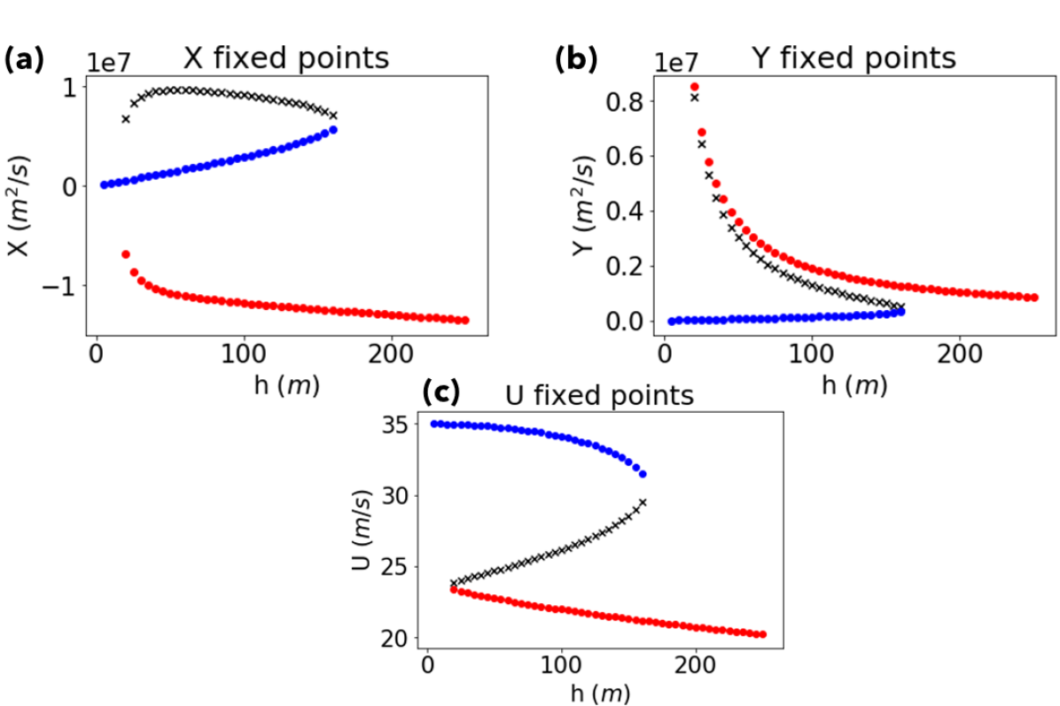
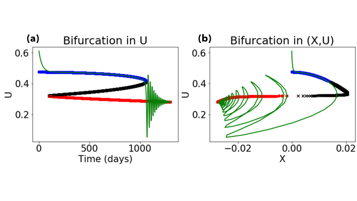
Remarkably, this hugely simplified model retains the qualitative structure of the Holton-Mass model as a bistable system for a certain range of between the critical values and , as shown in the bifurcation diagram of Figure 2. Blue points represent the normal state of the vortex, in approximate thermal wind balance with the radiative equilibrium temperature field (henceforth called the “radiative solution”). Red points represent a disturbed vortex, with weaker zonal wind and vacillations. This climatological regime supports more SSW events, and is henceforth called the “vacillating solution.” We use the same blue-red color scheme consistently here to represent these two states. Transitions between them happen on interannual time scales, affecting each year’s likelihood of SSW events. The structure of transitions is illustrated in Figure 3: as increases slowly past the bifurcation threshold , the system enters a series of rapid, large-amplitude oscillations that spiral into the weaker-circulation state.
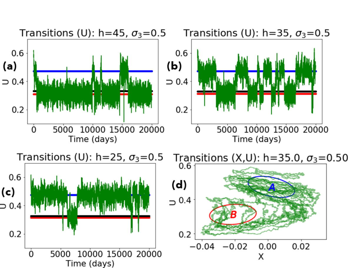
In Figures 2 and 3, transitions require crossing the bifurcation threshold , where the radiative solution ceases to exist. Birner and Williams (2008) introduced additive white-noise forcing in the variable to model unresolved gravity waves and found that these perturbations were sufficient to excite the system out of its normal state and into a vacillating regime. In Figure 4 we illustrate stochastic trajectories of the system for three different (fixed) values of . (For numerical reasons we also add a small amount of independent white noise to and variables). Even when is far below , transitions still occur, and in fact the preference for the vacillating solution branch increases quickly with .
Birner and Williams (2008) used direct numerical simulation and the Fokker-Planck equation to calculate long-term occupation statistics, i.e., how much time on average was spent in each regime and the mean first passage time before a transition to the vacillating regime, all for a range of forcing and noise levels. Our approach differs in both target and methodology. We aim to characterize the transition process between the two states, to monitor its progress in real time, as well as to describe statistics of the transition over many realizations. Methodologically, transition path theory phrases these questions in terms of the generator of the stochastic process, a differential operator that encodes all information about the behavior of the process.
3 Path properties
TPT characterizes the steady state statistics of transitions between states. In this section, we introduce key quantities needed to introduce TPT as applied to the Ruzmaikin model to obtain a more complete picture than we get from the sample paths shown above. For mathematical details, see the supplement and background literature (E and Vanden-Eijnden, 2006; Metzner et al., 2006; Vanden-Eijnden and E, 2010).
a. Infinitesimal Generator
The noisy Ruzmaikin model can be expressed compactly as a stochastic differential equation (SDE)—specifically a diffusion process—in the variable (or a more general phase space ) with a deterministic drift vector and a diffusion matrix .
| (17) |
Here, is a 3-vector of independent Brownian motions. We use the Ito convention for stochastic integration. While can in principle be any -dependent matrix, we make diagonal and constant: , creating independent additive noise in the , and variables. and have units of , while has units of . Associated with this equation is the infinitesimal generator , an operator describing the evolution of observable functions forward in time following a trajectory. Explicitly, if is a smooth function of phase space variables, then
| (18) |
where is an expectation over sample paths.
Ito’s lemma (the chain rule for diffusion SDEs) gives the Kolmogorov backward equation, which represents as a partial differential operator (for details see Pavliotis (2014)):
| (19) | ||||
| (20) |
The diffusion matrix is also called for convenience, which we will use interchangeably. denotes the Hessian matrix: . The generator provides path statistics as the solution to PDEs, as illustrated in the following subsections.
b. Equilibrium probability density
This stochastic process admits a time-dependent probability density, , which can be derived from the generator. For example, if the system starts in a known position , then . The density spreads out from this initial point over time according to the Fokker-Planck equation, which can be written in terms of the adjoint of the generator:
| (21) | |||
| (22) | |||
| (23) |
When is constant and diagonal, the last term simplifies to . In the case of pure Brownian motion, , then and , giving the heat equation (). Assuming that the process is ergodic, the density eventually forgets the initial condition and stabilizes into a long-term (or equilibrium, or stationary) probability density , which solves . This can be approximated by either simulating the SDE for a very long time and binning data points, or directly solving the stationary PDE , subject to the normalization and positivity constraints and .
c. Committor probability
The stationary density is an equilibrium quantity characterizing the long-term occupation statistics. But it is insufficient to describe the events of interest to us, which are transition paths: trajectory segments beginning inside the radiative state and ending inside the vacillating state. Specifically, we define the sets and as ellipsoids around these two fixed points, respectively. Their size is determined by contours of a local approximation to the stationary density ; see supplement for details. We say that a snapshot of the system is undergoing a transition (or reaction) at time if it is on the way from set to set . This involves information about both its future and its past, for which we introduce the forward and backward committor probabilities in this section.
The forward committor (denoted when context is clear) describes the progress of a stochastic trajectory traveling from set to set , as follows:
| (24) | ||||
| (25) |
The boundary conditions on and follow naturally from the probabilistic definition. If the system begins in set , by path continuity it will certainly next find itself in , with zero chance of hitting first. Starting in set the opposite is true. The committor therefore obeys the boundary value problem (see supplement for derivation)
| (26) |
The equivalence of conditional expectations with respect to a Markov process like the committor and solutions to PDE involving the generator of the process are generally referred to as Feynman-Kac relations (Karatzas and Shreve, 1998) and are well studied. The PDE in (25) is most naturally posed on an infinite domain, but as a numerical approximation we solve it in a large rectangular domain and impose homogeneous Neumann conditions at the domain boundary. A limiting example is the noise-dominated case, where is negligible and . The Kolmogorov backward equation then becomes Laplace’s equation:
| (27) |
If posed on the interval , with and , the solution is . The linear increase from set to set reflects the greater likelihood of entering when beginning closer to it. This limit is reflected in Figure 1, which shows the committor of the double-well potential approaching a straight line for large values.
Prediction is naturally much harder in high-dimensional systems such as stratospheric models. A number of physically interpretable fields, such as zonal wind and geopotential height anomalies, seem to have some predictive power for SSW, but prediction by any single such diagnostic is suboptimal. Insofar as they are successful, these variables approximate certain aspects of the committor. For example, the committor might increase monotonically with the quasi-biennial oscillation index. Furthermore, statistical correlations potentially obscure the conditional relationships needed. For example, Martius et al. (2009) and Bao et al. (2017) examined tropospheric precursors to SSW events in reanalysis records, finding that blocking events preceded most major SSWs, potentially by enhancing upward-propagating planetary waves. (We use “precursor” only to mean an event that sometimes happens before SSW.) Blocking influences SSW through height perturbations at the tropopause, which would enter the Ruzmaikin model as low-frequency variations in lower boundary forcing . Since we fix constant, the blocking precursor is outside our scope here. However, farther down the dynamic chain are other measurable precursors such vertical wave activity flux and meridional heat flux, which are also found to have predictive power (Sjoberg and Birner, 2012). However comprehensive the model, we would naturally expect the true committor probability to exhibit similar patterns to canonical precursors of that model such as blocking (for a troposphere-coupled model) and heat flux (for a stratosphere-only model). Yet, there is an important difference: while a precursor may appear with high probability given that a SSW is imminent, the committor specifies the probability of a SSW given an observed pattern. As acknowledged in Martius et al. (2009), many blocking events did not lead to SSW events, meaning that . Such distinctions highlight the need for a precise mathematical formulation that provides and distinguishes both kinds of information.
While describes the future of a transition, the backward committor describes its past. It is defined as
| (28) | ||||
| (29) |
solves the time-reversed Kolmogorov backward equation , where is the time-reversed generator, which evolves observables backward in time. See supplement for a detailed description of and its relationship the forward generator .
We now describe the fundamental statistics characterizing transition events as identified by TPT and explain how they can be expressed in terms of quantities such as , , and . The probability density of reactive trajectories , the probability of observing the system at the location during a transition, is proportional (up to a normalization constant) to the product . This density is large in regions of phase space that are highly trafficked by reactive trajectories. This is how TPT gives information about precursors, indicating regions of phase space that are usually visited by the system over the course of a transition path.
The direction and intensity of this traffic is specified by the reactive current. To develop this concept, we start by introducing the probability current , a vector field that satisfies a continuity equation with the time-dependent density :
If were the density and the velocity field of a fluid, would be . One can think of as an instantaneous (in time and position) average over all possible system trajectories, though a precise mathematical description requires some care. In equilibrium, when is no longer changing, , or equivalently where is any closed surface.
The reactive current is also an “average velocity”, but restricted to reactive paths. Unlike , is not divergence-free, with a source in and a sink in (where transition paths start and end). is defined implicitly via surface integrals. If is any surface enclosing set but not set , with outward normal , then the flux is the number of forward transitions per unit time, also called the transition rate ; see Vanden-Eijnden and E (2010) for details. The supplement describes another expression in terms of the generator. The result is (Metzner et al., 2006)
| (30) | ||||
| (31) |
where again is the stationary density. This expression has intuitive ingredients. Multiplying by conditions the equilibrium probability current on the trajectory being reactive, meaning en route from to . The reflects the fact that trajectories from to must ascend a gradient of , going from to , while descending a gradient of .
Just as describes the average reactive velocity, a streamline of (solving , with and for some ) is a kind of “average” transition path. Although the streamline will not be realized by any particular transition path, it will have common geometric features in phase space with many actual path samples. At low noise the reactive trajectories will cluster in a thin corridor about the streamline. The streamline is a more dynamical description of precursors: whereas regions of high reactive density are commonly observed states along reactive trajectories, streamlines of reactive current are commonly observed sequences of states along reactive trajectories. The study by Limpasuvan et al. (2004), for example, described a sequence of events in a prototypical SSW life cycle based on reanalysis including vortex preconditioning, wave forcing, and anomalous heat fluxes at various levels in the troposphere and stratosphere. The sequence described there likely corresponds to a streamline of the reactive trajectory.
The committor also quantifies the relative balance of time spent on the way to each set. If more probability mass lies in the region where , set is globally more imminent, whereas more mass where indicates set is. A single summary statistic of imminence is the average committor during a long trajectory, , computed as a weighted average against the equilibrium density:
| (32) |
An average below (above) would indicate more time spent on the way to to ().
Another statistic, the forward transition rate, captures the frequency of transitions between and rather than the overall time spent in each. We earlier defined as the number of transitions per unit time. Since a transition must occur between every two transitions, . The inverse of the transition rate is the return time, a widely used metric for changing frequency of extreme events under climate change scenarios (Easterling et al., 2000). However, the forward and backward transitions may differ in important characteristics like speed. To capture this asymmetry, we need a dynamical analogue to the equilibrium statistic . The typical quantity of choice is the rate constant , which is larger if transitions happen faster than transitions. We therefore normalize by the overall time spent having come from , which is .
| (33) |
This rate constant, defined in Vanden-Eijnden (2014), parallels the chemistry definition. If and are two chemical species, with denoting concentration, the forward and backward rate constants and are defined so that
| (34) |
In the language of transition path theory, is the long-term probability of the system existing most recently in state , which is . Rates are also expressible in terms of expected passage times. Thinking of as the total probability of having last visited set , estimates the total transition time between entering (having last visited ) and next re-entering . It is these inverse quantities we display in the results section.
These quantities together make an informative description of the typical transition process from to . We now proceed to analyze the transition path properties of the Ruzmaikin stratospheric model.
4 Methodology
a. Spatial discretization
The quantities of interest described above (, , , and ) emerge as solutions to PDEs involving the generator , which must be approximated by spatial discretization. In the supplement we describe a finite volume scheme to directly discretize the adjoint as a matrix, which we name , on a regular grid in dimensions. Here we use the same domain and noise levels as Birner and Williams (2008): , , in units non-dimensionalized in terms of the radius of Earth and the length of a day. We tile this with a grid of grid cells. We choose a noise constant in the variable in the range . This is a similar range to observed atmospheric gravity wave momentum forcing (Birner and Williams, 2008). For numerical reasons, we also add small noise to the streamfunction variables and , in proportion to the domain size. Specifically, as spans a range of and span a smaller range of , we choose and to be . This adjustment does change our results with respect to Birner and Williams (2008), causing more transitions in both directions at lower than if only the variable were perturbed. While gravity wave drag forces the zonal wind, eddy interactions and other sources of internal variability can perturb the streamfunction as well, and it is not uncommon to represent these effects stochastically (DelSole and Farrell, 1995). There are surely more accurate representations of noise, but this important issue is not our focus. We retain these perturbations for numerical convenience, but stress that the general principles of the TPT framework are independent of any specific form of stochasticity. In the forthcoming experiments, we will refer only to with the understanding that and are adjusted proportionally. The discretization we use has strengths and limitations. Given the matrix on this grid, the discretized generator is just the transpose. To ensure certain properties of solutions, such as positivity of probabilities, should ideally retain characteristics of the infinitesimal generator of a discrete-space, continuous-time Markov process: rows that sum to zero, and nonnegative off-diagonal entries. Such a discretization is called “realizable” (Bou-Rabee and Vanden-Eijnden, 2015). One can check that our discretization always satisfies the former property, and so is realizable provided small enough grid spacing . In our current example, the spacing is not nearly small enough to guarantee this (matrix entries were just as often negative as positive), but results are still accurate, as verified by stochastic simulations to be described in the results section. While we could have used one-sided finite differences to enforce positivity, this would have degraded the overall numerical accuracy of the solutions. We opted instead to zero out negatives, which were always negligible in magnitude.
The discretized Kolmogorov backward equation is , augmented with appropriate boundary conditions. The definition of and is a design choice that should satisfy three conditions: (1) they are disjoint, (2) contains the radiative fixed point and the fixed point of the vacillating regime, and (3) both sets are relatively stable in the chosen noise range. We choose and to be ellipses with orientations determined by the covariance of the equilibrium density of the linearized stochastic dynamics about their respective fixed points, as described in the supplement. The choice of the sizes of and is a subjective decision which alters the very definition of a reactive trajectory; hence, different sizes emphasize different features of the transition path ensemble, especially in oscillatory systems like this one. We made and large enough to enclose the many loops that often accompany the escape from and the descent into , so that we can focus on the relatively rare crossing of phase space. More sophisticated techniques exist for shrinking the two sets while erasing resulting loops (Lu and Vanden-Eijnden, 2014; Banisch and Vanden-Eijnden, 2016); for simplicity, we forgo these techniques for the current study.
Careful discretization is important for constructing the dominant pathways discussed above, i.e. the streamlines satisfying . Standard integration techniques such as Euler or Runge-Kutta will accumulate errors, not only from Taylor expansion but also from the discretized solution of , and . These can be severe enough to prevent from reaching set . To guarantee that full transitions are extracted, we instead solve shortest-path algorithms on the graph induced by the discretization, as described in Metzner et al. (2009). The supplement contains more details on this computation.
5 Results
We begin this section by describing the kinematic path characteristics of the process in its three-dimensional phase space, according to the quantities described above. Following this purely geometrical description, we will suggest some dynamical interpretations and compare with previous studies. Finally, we will map statistical features as functions of background parameters.
The Ruzmaikin model is attractive for demonstrating use of the tools introduced in Section 3 due to its low-dimensional state space, in which PDEs can be solved numerically using standard methods such as our finite volume scheme. We tested the committor’s accuracy empirically by randomly selecting 50 cells in our grid (this is of the grid) and evolving stochastic trajectories forward in time from each, stopping when they reach either set or set . The fraction of trajectories starting from that first reach is taken as the empirical committor at point and is denoted , which we compare with the predicted committor from the finite volume scheme. Figure 5 clearly demonstrates the usefulness of the committor for probabilistic forecasting. The left column displays the committor calculated from finite volumes, averaged in the direction, for two different forcing levels . The right column shows a scatterplot of vs. at the 50 randomly selected grid cells. We expect the points to fall along the line with some spread proportional to the standard deviation of the binomial distribution, . Approximating this as a Gaussian, we have plotted red curves enclosing the 95% confidence interval, which indeed contains approximately 95% of the data points. Statistical sampling error can explain the observed level of deviation, although discretization error (from solving the PDE and from time-stepping) may also contribute.
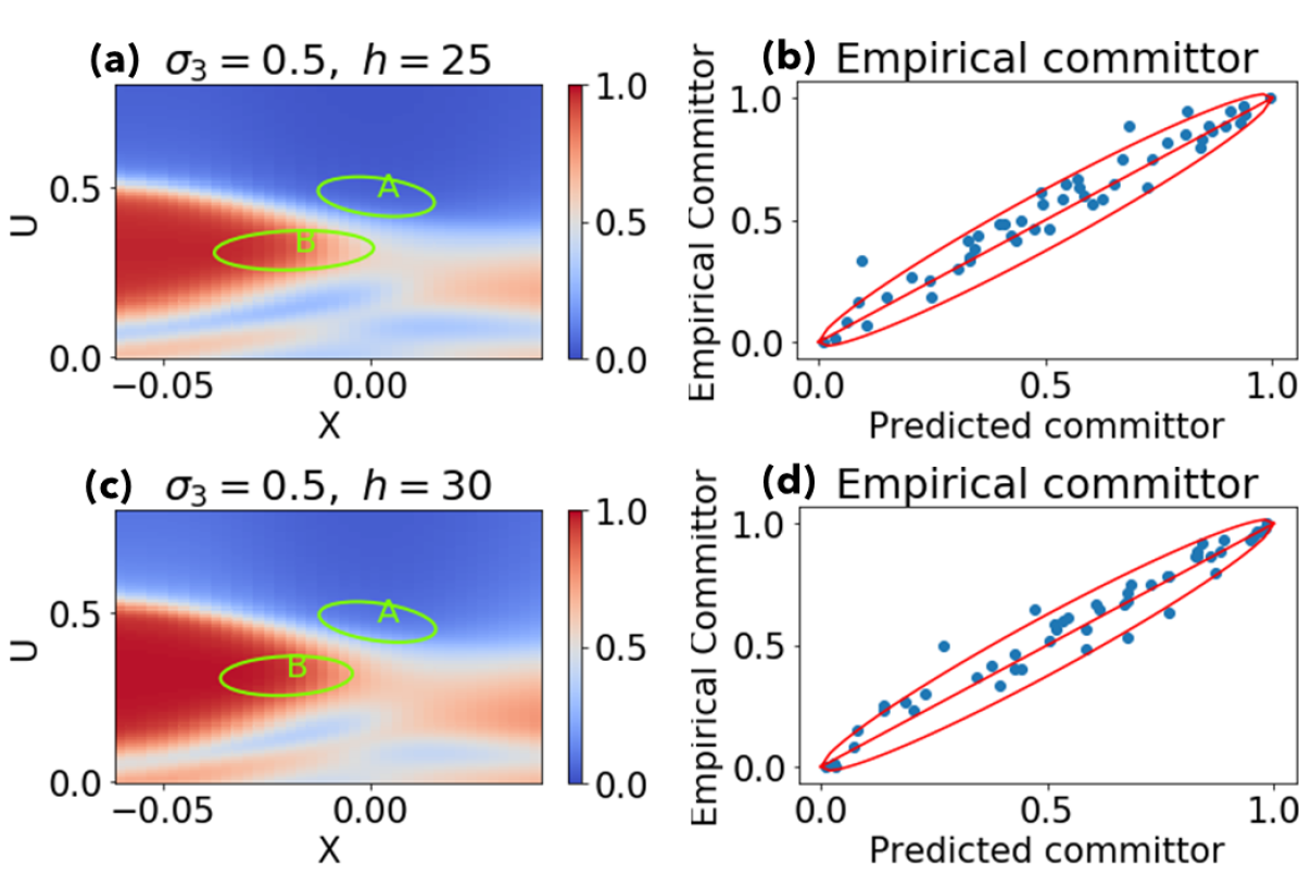
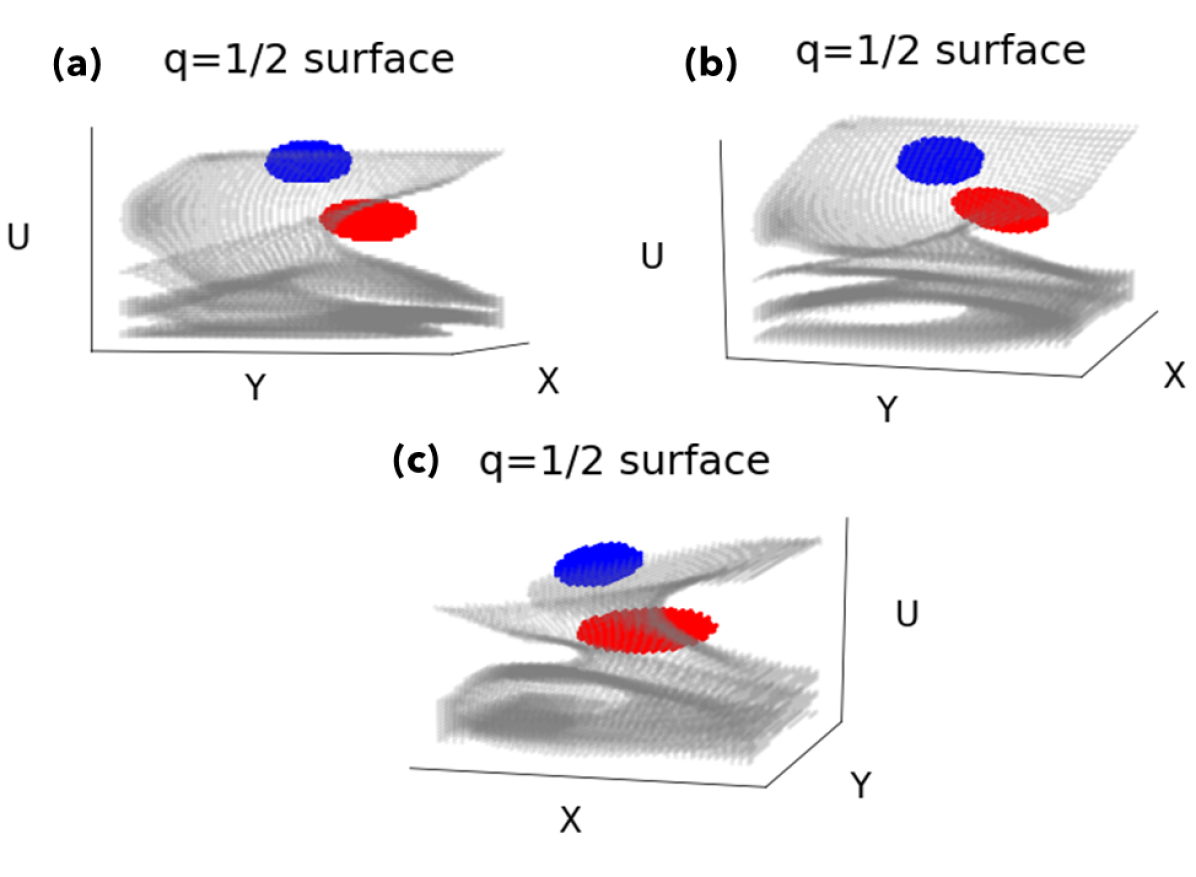
Figure 5 also shows how responds to increasing , even far below the bifurcation threshold: the committor values throughout state space become rapidly skewed toward unity (meaning more red in the picture). This means that even slight perturbations can kick the system out of state toward state . Another indicator is the “isocommittor surface”, the set of points such that ; that is, the system has equal probability of next entering set or . In the left-hand column this is the set of gray points (averaging out the variable Y). For low forcing, this surface tightly encloses set , meaning the system must wander very close before a transition is imminent. For high forcing values, the isocommittor hugs set more closely, meaning that small perturbations from this normal state can easily push the system into dangerous territory. In Figure 6, the isocommittor is shown as a set of gray points in a 3D plot viewed from various vantage points. In the low- region, the isocommittor resembles a spiral staircase, reflecting the spiral-shaped stable manifold of the fixed point in set . Different initial positions with the same streamfunction phase, differing only slightly in the direction, can have drastically different final destinations. These spiral surfaces are responsible for the blue lobes in the lower part of Figure 5, but they disappear at higher noise.
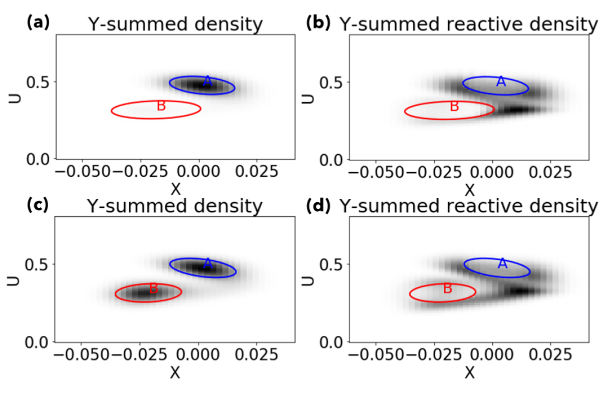
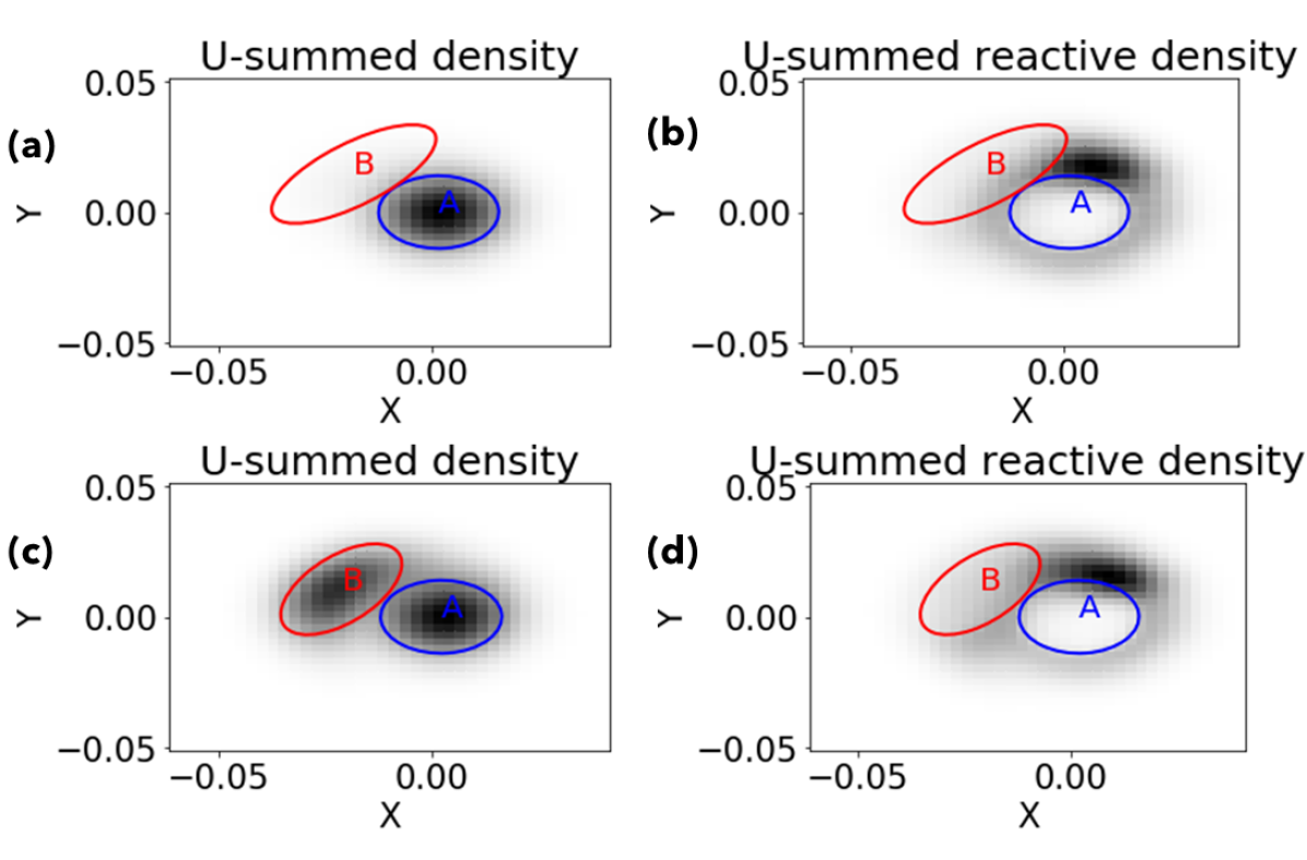
Figures 7 and 8 display numerical solutions of the equilibrium density and reactive density for two forcing levels. While indicates where tends to reside, indicates where resides given a transition from to is underway. As increases, even far below the bifurcation threshold, responds strongly, shifting weight toward state . On the other hand, the reactive density displays similar characteristics for all values. In the plane, the two lobes of high reactive density surrounding indicate that zonal wind tends to remain strong for a while before dipping into the weaker regime. Viewing the same field in the plane (Figure 8) reveals a halo of intermediate density about set . While many different motions would be consistent with this pattern, the coming figures verify that the early stages of transition have circular loops in the plane, meaning zonal movement of the streamfunction’s peaks and troughs. The exact streamfunction phase corresponding to the position is calculated as follows. Recall the streamfunction is , where . In polar coordinates, , where . The full streamfunction is
where is longitude.
The angle from the origin in the plane indicates the zonal streamfunction phase, and circular motion indicates zonal movement. (This “looping” motion is indeed shared by the transition path samples shown in Figures 9 and 10, to be described later.)
The darkest (most-trafficked) region of this loop is the sector . The relationship between and indicates is maximized at longitudes . As the maximum reactive density occurs around , the streamfunction peaks are at . What is the significance of this phase relative to the lower boundary forcing? Recalling the forcing form , the bottom peaks are located at . Hence, the bulk of the transition process happens when the perturbation streamfunction at the mid-stratosphere lags the lower boundary condition by of a wavelength. Meanwhile, the plane reveals what happens to the zonal wind speed during the SSW transition. The high-reactive density region discussed above coincides with the crescent-shaped bridge of high density between the sets in Figure 7. This suggests that in an SSW, the zonal wind weakens while the streamfunction stays in that particular phase window.
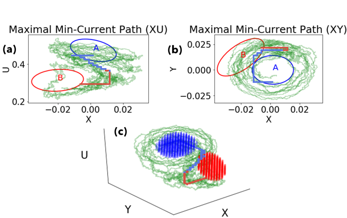
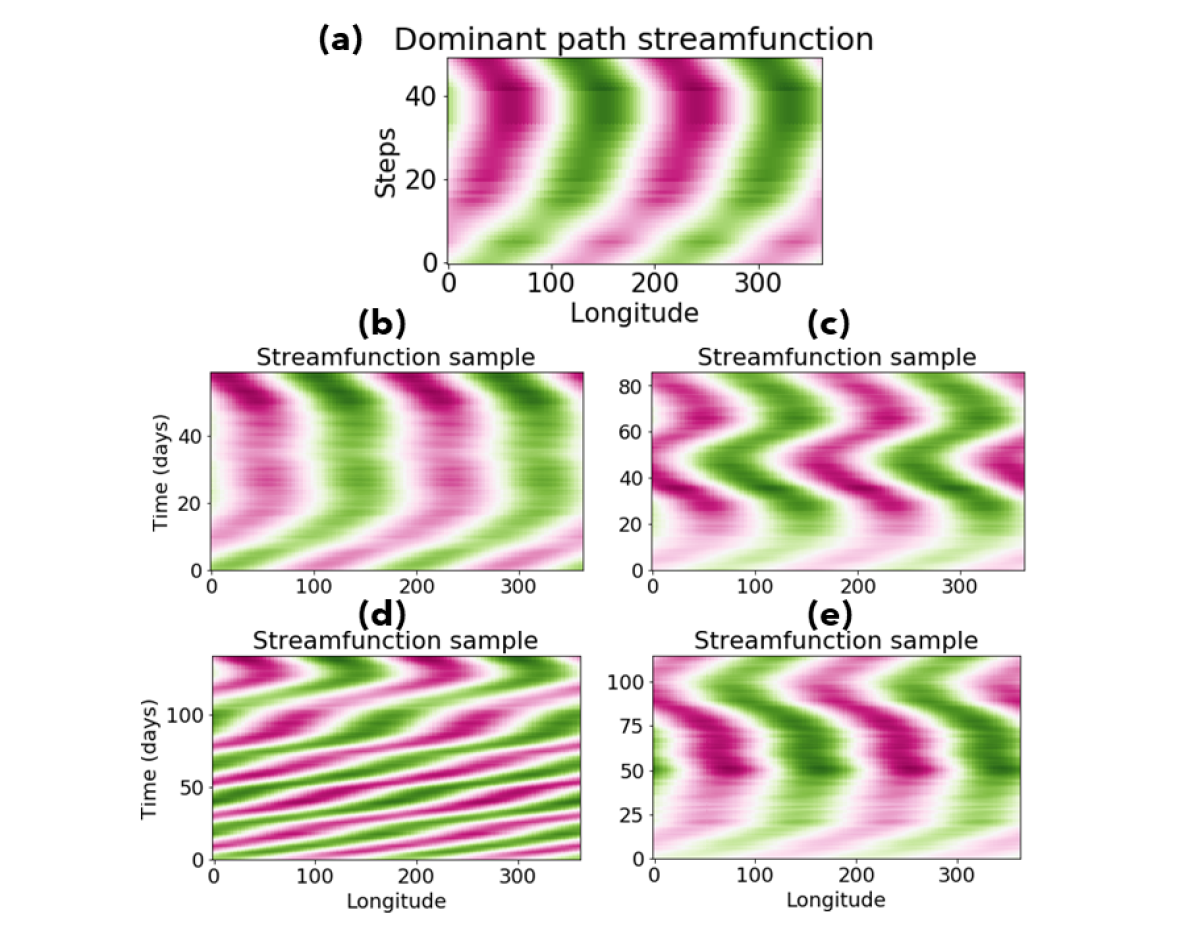
The pictures of reactive density suggest that reactive trajectories tend to loop around set , physically meaning the streamfunction tends to travel in one direction before slowing down, but they technically convey no directional information to explicitly support this claim. For this, we turn to the reactive current. We computed the discrete-space effective current matrix , directly from the finite volume discretization and numerical solutions of , and . Physically, this matrix represents the flux of a vector field from grid cell to cell . From this we calculated the maximum-current paths as described in Metzner et al. (2009) and displayed the results in Figure 9 for a forcing level of (other levels are qualitatively similar). Both the and views are shown. Superimposed on these paths are seven actual reactive trajectories that occurred during a long stochastic simulation, to demonstrate features that are captured by the dominant pathways. The dominant path from to indeed contains a half-loop in the plane in the clockwise direction, which means an eastward phase velocity. With a smaller set , this dominant path would contain more of these loops. However, during the next transition stage, the streamfunction slows to a halt at the phase angle , doubles back and travels westward as zonal wind loses strength. The smear of high density in the neighborhood therefore comprises not only a precipitous drop in zonal wind (which happens at the edge of that region) but also a backtrack, this time with weaker background zonal wind. This behavior is borne out by the trajectory samples, which vacillate in the upper-middle section of the plot. These paths are displayed as space-time diagrams of the streamfunction in Figure 10. In panel (a), the dominant path’s two loops correspond to two troughs moving east past a fixed longitude before the slowdown. The random streamfunction trajectories shown in (b)-(g) do not follow this representative history exactly, but they do combine elements of it: steady eastward wave propagation followed by slowdown and reversal. Each stage can have multiple false starts. Notably, the slowdown consistently happens at the same phase, with peaks at and , at roughly the same phase as found from the density plots. In fact, the figures show a brief slowdown every time the streamfunction passes this phase. This can be thought of as a representation of blocking events that often accompany sudden stratospheric warmings. The third transition path shown is an exception to the general pattern, making a final turn toward the east instead of to the west. This outlier of a reactive trajectory can also be seen in Figure 9, as the single green trajecory that decreases in before decreasing in instead of the other way around.
This kinematic sequence of events has a dynamical interpretation with precedent in prior literature. A critical ingredient of SSW is meridional eddy heat flux, which in this model takes the form (see the supplement for a detailed derivation.) This term shows up explicitly as a negative forcing on in equation (15), showing that a reduced equator-to-pole temperature gradient in turn weakens the vortex via the thermal wind relation. The association of heat flux with SSW has been demonstrated in reanalysis (Sjoberg and Birner, 2012) and in detailed numerical simulations of internal stratospheric dynamics, even with time-independent lower boundary forcing (Scott and Polvani, 2006). This relationship favors the phase as the most susceptible state for SSW onset, which is exactly picked out by the dominant transition pathway in Figure 9.
However, immediately after the wind starts weakening at , where the streamfunction lines up with its lower boundary condition, the phase velocity reverses, giving rise to the westward lag of we observed in the reactive density. A similar phase lag has also been observed in more detailed numerical studies. For example, Scott and Polvani (2006) observed a lag of across the whole stratosphere ( at the mid-level), quite similar to our result. They found that vortex breakup was preceded by a long, slow build-up phase in which the vortex became increasingly vertically coherent, only to be ripped apart by an upward- and west-propagating wave. In an experiment with slowly-increasing lower boundary forcing, Dunkerton et al. (1981) saw a phase lag across the whole stratosphere that increased from to ( to between the lower boundary and the mid-stratosphere) over the course of the warming event. They attribute this phase tilt to the zonal wind rapidly reversing and carrying the streamfunction along. The weakening zonal wind simply removes the Doppler shift from the Rossby wave dispersion relation, , allowing the waves to revert to their preferred westward phase velocity. This balance is also clear in equations (13-14): ignoring the damping and forcing terms, the dynamics read . For weak , rotation in the plane is anti-clockwise and phase speed is westward.
Let us re-emphasize the probabilistic interpretation of reactive density. We have found that transitions from to are accompanied by anomalous increases in meridional heat flux. In other words, is high. As noted earlier, this does not imply that is also high. The identified streamfunction phase is not a “danger zone” in the sense that a trajectory entering this region is at higher risk of falling into state ; the committor alone conveys that information. Rather, a trajectory is highly likely to pass through that region given that it is reactive. Notably, reactive trajectories are unlikely to take a straight-line path from to with , and changing linearly. This unrealistic path would represent a zonally stationary streamfunction growing steadily in magnitude, while zonal wind falls off gradually. At higher noise levels, however, the system would be increasingly dominated by pure Brownian motion, and such a path would become more plausible.
We now turn to a quantitative comparison of committors and transition rates for different forcing and noise levels. These trends illustrate the effects of modeling choices and global change on the climatology of SSW. Planetary wave forcing, , varies across days and seasons as well as different planets. The strength of additive noise, , is a modeling choice intended to represent gravity wave drag. Different stochastic parametrizations will vary in their effective value, and it is important to understand the sensitivity of SSW to model choices (Sigmond and Scinocca, 2010). Furthermore, long-term climate change may cause both parameters to drift, altering the occurrence of SSW-induced severe weather events.
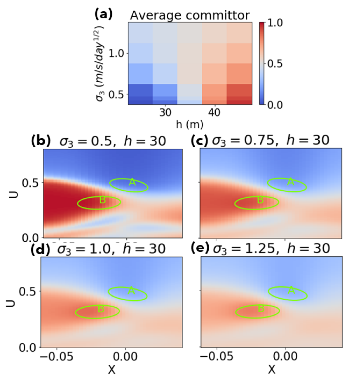
The measure of the relative “imminence” of a vacillating solution vs. a radiative solution, as described in the background section on committors, is the equilibrium density-weighted average committor, denoted . Figure 11(a) shows this quantity for () and (. Two trends are clearly expected from the basic physics of the model. First, as seen in Figures 7 and 8, should increase with . Second, in the limit of large noise and infinite domain size, the dominance of Brownian motion will smooth out the committor function and make tend to an intermediate value between zero and one. On the other hand, as noise approaches zero, the dynamical system becomes increasingly deterministic, and the ultimate destination of a trajectory will depend entirely on which basin of attraction it starts in. The boundary, or separatrix, between these two basins is the stable manifold of the third (unstable) fixed point. In the case of a potential system, of the form , this boundary would be a literal ridge of the function . Our system admits no such potential function, but this is a useful visual analogy. The committor function becomes a step function in the deterministic limit, with the discontinuity located exactly on this boundary. The addition of low noise moves the committor- surface away from the separatrix, possibly asymmetrically: one basin will shrink, becoming more precarious with respect to random perturbations, while the other will expand, becoming a stronger global attractor. Which basin will shrink is not evident a priori, so we compute the averaged committor, , as a summary statistic which will increase when the basin of expands.
Figure 11(a) plots the trends in as a function of (along the horizontal axis) and (along the vertical axis). The two basic hypotheses are verified: increases monotonically as increases, and as increases, no matter the value of . The less predictable behavior is in the range , , where displays non-monotonicity with respect to noise, at low noise levels. As increases, the average committor increases from to , and then decreases again. The four committor plots at the bottom of 11 illustrate the trend graphically. At low noise, the basin includes winding passageways leading from the small- region back to . Small additive noise closes them off, effectively expanding the basin. As noise increases and Brownian motion dominates the dynamics, committor values everywhere relax back to less-extreme values, reflecting the unbiased nature of Brownian motion.
Despite the coarse grid resolution, the first-order effect of noise is clear. At the low and high margins of , where falling into state and respectively is virtually certain, an increase in noise decreases this virtual certainty, and the trend continues at larger noise to attenuate to its limit of 1/2. The middle range, however, behaves differently. Whereas appears to balance out the basin sizes at low noise, a slight noise increase tends to kick the system out of the basin and toward , more so than the other way around. At higher noise, the committor relaxes back to 1/2. Examining the committor fields, it’s clear that the isocommittor surface location does not move back and forth; rather, it moves toward , and then the rest of the field flattens out.
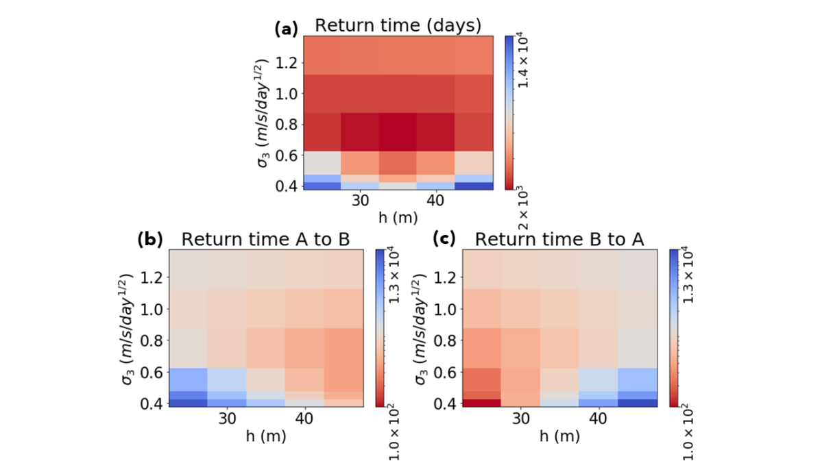
Figure 12 shows trends in the return times of SSW with varying and . There are several different return times of interest. The first, shown in panel (a), is the total expected time between one transition event and the next, whose reciprocal is the rate , the number of transitions per unit time. The return time is a symmetric quantity between and , since every forward transition is accompanied by a backward one. Among the parameter combinations, is the one which minimizes return time, or equivalently maximizes the transitions per unit time. is a forcing level which approximately balances out the time spent between the two sets, making transitions relatively common. At lower noise, transitions are exceedingly rare, and at higher noise the two states cease to be long-lived. However, this symmetric quantity does not capture information about the relative speed of transition from to vs. from back to . Panel (b) shows a different passage time, which is the average time between the end of a backward transition and the end of the next forward () transition, which we call . This is computed as the reciprocal of the rate constant , as described in the previous section. In other words, the stopwatch begins when the system returns to after having last visited , and ends when the system next hits . This metric is asymmetric: a smaller return time indicates that the forward transition is faster than the backward transition. Panel (b) shows the complementary return time, . Unsurprisingly, an increase in causes a decrease in and an increase in regardless of the noise level. The noise level has a less obvious effect. Whereas decreases monotonically with increasing noise, regardless of , the forward time is minimized by a mid-range noise level of . This is another reflection of the bias toward state that is effected by adding noise to a very low baseline.
6 Conclusion
Transition path theory is a framework for describing rare transitions between states. We have described TPT along with a number its key ingredients like the forward and backward committor functions. While TPT has been applied primarily to molecular systems, we believe it offers valuable insight into climate and weather phenomena such as sudden stratospheric warming, primarily through committors, reactive densities, and reactive currents. Of interest apart from its role in TPT, the forward committor defines an optimal probabilistic forecast, borne out by direct numerical simulation experiments. The reactive densities and currents describe the geometric properties of dominant transition mechanisms at low noise. In applying TPT to a noisy, truncated Holton-Mass model, we find that transitions tend to begin with a drop in mean zonal wind and a reversal of the streamfunction’s phase velocity at a particular streamfunction phase. This is consistent with the significance of blocking precursors to SSW as found in Martius et al. (2009), insofar as this idealized model can represent them. We also find that noise has a non-monotonic effect on the overall preference for a vacillating state, measured by the average committor. At a forcing of , where the isocommittor surface (essentially the basin boundary of the deterministic dynamics) divides the space approximately in half, we find that raising the noise tilts the balance decisively toward the vacillating solution. Still larger noise evens the whole field out. The transition rate constant shows a similar dependence on and .
In future work, we plan to scale these methods to more realistic and complex models as well as observational data, where predicting SSW remains an active area of research. In this high-dimensional setting, the generator may be unknown or computationally intractable. Any state space with more than degrees of freedom is beyond the reach of a finite-volume discretization, because the number of grid cells increases exponentially with dimension. However, there is a generic insight that physical models evolve on very low-dimensional manifolds within the full available state space. A growing body of research in molecular dynamics (Thiede et al., 2019), fluid dynamics (Giannakis et al., 2018; Froyland and Junge, 2018), climate dynamics (Giannakis and Majda, 2012; Sabeerali et al., 2017), and general multiscale systems (Harlim and Yang, 2018; Berry et al., 2015; Giannakis, 2015, 2019) exploits the intrinsic low-dimensionality to represent the infinitesimal generator more efficiently. While here we represented the generator as a finite-volume or finite-difference operator on a grid, one can also write it in a basis of globally coherent functions, such as Fourier modes, or more generally harmonic functions on a manifold. Given only data, without an explicit form of the dynamics, this manifold and the basis functions can be estimated from (for example) the diffusion maps algorithm, and the generator’s action on this basis can be approximated from short trajectories. These ideas can be applied to computing the dynamical statistics that have been the focus of this paper (Thiede et al., 2019). We hope that these techniques will enable more efficient observation strategies for targeted data assimilation procedures with the goal of tracking the progression of specific extreme events, including hurricanes and heat waves as well as sudden stratospheric warming.
Data from this study will be made available upon request.
Acknowledgements.
Justin Finkel was funded by the Department of Energy Computational Science Graduate Fellowship under grant DE-FG02-97ER25308. We acknowledge support from the National Science Foundation under NSF award number 1623064. Jonathan Weare was supported by the Advanced Scientific Computing Research Program within the DOE Office of Science through award DE-SC0020427. The reviewers of the paper provided invaluable insights on physical interpretation of the mathematical results. In particular, they helped us to recognize the connection between our computed maximum-flux reactive pathway and anomalous heat fluxes which weaken the zonal wind and reverse the streamfunction’s phase velocity. We thank Cristina Cadavid, Thomas Birner and Paul Williams for helpful clarifications about previous work. We thank Eric Vanden-Eijnden, Mary Silber, Robert Webber, Erik Thiede, Aaron Dinner, Tiffany Shaw, and Noboru Nakamura for useful discussions throughout this project. The University of Chicago’s Research Computing Center provided the computational resources to greatly expedite the calculations done here. Below are the numerical coefficients used in the reduced-order Ruzmaikin model, with very similar values to Ruzmaikin et al. (2003) and Birner and Williams (2008). The relationship with physical parameters is described in the appendix of Ruzmaikin et al. (2003). Note that our notation differs slightly: following Birner and Williams (2008), we write the topographic forcing in terms of rather than , a difference that results in numerical factors of depending on the convention used.| (35) | ||||
| (36) | ||||
| (37) | ||||
| (38) | ||||
| (39) | ||||
| (40) | ||||
| (41) | ||||
| (42) | ||||
| (43) | ||||
| (44) | ||||
| (45) |
References
- Albers and Birner (2014) Albers, J. R., and T. Birner, 2014: Vortex preconditioning due to planetary and gravity waves prior to sudden stratospheric warmings. Journal of the Atmospheric Sciences, 71 (11), 4028–4054, 10.1175/JAS-D-14-0026.1.
- Baldwin and Dunkerton (2001) Baldwin, M. P., and T. J. Dunkerton, 2001: Stratospheric harbingers of anomalous weather regimes. Science, 96 (5542), 581–584, 10.1126/science.1063315.
- Bancalá et al. (2012) Bancalá, S., K. Krüger, and M. Giorgetta, 2012: The preconditioning of major sudden stratospheric warmings. Journal of Geophysical Research: Atmospheres, 117 (D4), 10.1029/2011JD016769.
- Banisch and Vanden-Eijnden (2016) Banisch, R., and E. Vanden-Eijnden, 2016: Direct generation of loop-erased transition paths in non-equilibrium reactions. Faraday Discussions, 195, 443–468, 10.1039/c6fd00149a.
- Bao et al. (2017) Bao, M., X. Tan, D. L. Hartmann, and P. Ceppi, 2017: Classifying the tropospheric precursor patterns of sudden stratospheric warmings. Geophysical Research Letters, 44 (15), 8011–8016, 10.1002/2017GL074611.
- Berry et al. (2015) Berry, T., D. Giannakis, and J. Harlim, 2015: Nonparametric forecasting of low-dimensional dynamical systems. Phys. Rev. E, 91, 032 915, 10.1103/PhysRevE.91.032915.
- Birner and Williams (2008) Birner, T., and P. D. Williams, 2008: Sudden stratospheric warmings as noise-induced transitions. Journal of the Atmospheric Sciences, 65 (10), 3337–3343, 10.1175/2008JAS2770.1.
- Bou-Rabee and Vanden-Eijnden (2015) Bou-Rabee, N., and E. Vanden-Eijnden, 2015: Continuous-time random walks for the numerical solution of stochastic differential equations. Memoirs of the American Mathematical Society.
- Bowman et al. (2009) Bowman, G. R., K. A. Beauchamp, G. Boxer, and V. S. Pande, 2009: Progress and challenges in the automated construction of markov state models for full protein systems. The Journal of chemical physics, 131 (12), 124 101.
- Butler et al. (2015) Butler, A. H., D. J. Seidel, S. C. Hardiman, N. Butchart, T. Birner, and A. Match, 2015: Defining sudden stratospheric warmings. Bulletin of the American Meteorological Society, 96 (11), 1913–1928, 10.1175/BAMS-D-13-00173.1.
- Charlton and Polvani (2007) Charlton, A. J., and L. M. Polvani, 2007: A new look at stratospheric sudden warmings. part i: Climatology and modeling benchmarks. Journal of Climate, 20 (3), 449–469, 10.1175/JCLI3996.1.
- Chodera and Noe (2014) Chodera, J. D., and F. Noe, 2014: Markov state models of biomolecular conformational dynamics. Current Opinion in Structural Biology, 25, 135–144, https://doi.org/10.1016/j.sbi.2014.04.002.
- Christiansen (2000) Christiansen, B., 2000: Chaos, quasiperiodicity, and interannual variability: Studies of a stratospheric vacillation model. Journal of the Atmospheric Sciences, 57 (18), 3161–3173, 10.1175/1520-0469(2000)057¡3161:CQAIVS¿2.0.CO;2.
- DelSole and Farrell (1995) DelSole, T., and B. F. Farrell, 1995: A stochastically excited linear system as a model for quasigeostrophic turbulence: Analytic results for one- and two-layer fluids. Journal of the Atmospheric Sciences, 52 (14), 2531–2547, 10.1175/1520-0469(1995)052¡2531:ASELSA¿2.0.CO;2.
- Dematteis et al. (2018) Dematteis, G., T. Grafke, and E. Vanden-Eijnden, 2018: Rogue waves and large deviations in deep sea. Proceedings of the National Academy of Sciences, 115 (5), 855–860, 10.1073/pnas.1710670115.
- Dunkerton et al. (1981) Dunkerton, T., C.-P. F. Hsu, and M. E. McIntyre, 1981: Some eulerian and lagrangian diagnostics for a model stratospheric warming. Journal of the Atmospheric Sciences, 38 (4), 819–844, 10.1175/1520-0469(1981)038¡0819:SEALDF¿2.0.CO;2.
- Durrett (2013) Durrett, R., 2013: Probability: Theory and Examples. Cambridge University Press.
- E and Vanden-Eijnden (2006) E, W., and E. Vanden-Eijnden, 2006: Towards a theory of transition paths. Journal of Statistical Physics, 123 (3), 503–523, 10.1007/s10955-005-9003-9.
- Easterling et al. (2000) Easterling, D. R., G. A. Meehl, C. Parmesan, S. A. Changnon, T. R. Karl, and L. O. Mearns, 2000: Climate extremes: Observations, modeling, and impacts. Science, 289 (5487), 2068–2074, 10.1126/science.289.5487.2068.
- Franzke and Majda (2006) Franzke, C., and A. J. Majda, 2006: Low-order stochastic mode reduction for a prototype atmospheric gcm. Journal of the Atmospheric Sciences, 63 (2), 457–479, 10.1175/JAS3633.1.
- Froyland and Junge (2018) Froyland, G., and O. Junge, 2018: Robust fem-based extraction of finite-time coherent sets using scattered, sparse, and incomplete trajectories. SIAM Journal on Applied Dynamical Systems, 17 (2), 1891–1924, 10.1137/17M1129738.
- Giannakis (2015) Giannakis, D., 2015: Dynamics-adapted cone kernels. SIAM Journal of Applied Dynamical Systems, 14, 556–608, 10.1137/140954544.
- Giannakis (2019) Giannakis, D., 2019: Data-driven spectral decomposition and forecasting of ergodic dynamical systems. Applied and Computational Harmonic Analysis, 47 (2), 338 – 396, https://doi.org/10.1016/j.acha.2017.09.001.
- Giannakis et al. (2018) Giannakis, D., A. Kolchinskaya, D. Krasnov, and J. Schumacher, 2018: Koopman analysis of the long-term evolution in a turbulent convection cell. Journal of Fluid Mechanics, 847, 735–767, 10.1017/jfm.2018.297.
- Giannakis and Majda (2012) Giannakis, D., and A. J. Majda, 2012: Nonlinear laplacian spectral analysis for time series with intermittency and low-frequency variability. Proceedings of the National Academy of Sciences, 109 (7), 2222–2227, 10.1073/pnas.1118984109, https://www.pnas.org/content/109/7/2222.full.pdf.
- Harlim and Yang (2018) Harlim, J., and H. Yang, 2018: Diffusion forecasting model with basis functions from qr-decomposition. Journal of Nonlinear Science, 28 (3), 847–872, 10.1007/s00332-017-9430-1.
- Hasselmann (1976) Hasselmann, K., 1976: Stochastic climate models part i. theory. Tellus, 28 (6), 473–485, 10.3402/tellusa.v28i6.11316.
- Hoffman et al. (2006) Hoffman, R. N., J. M. Henderson, S. M. Leidner, C. Grassotti, and T. Nehrkorn, 2006: The response of damaging winds of a simulated tropical cyclone to finite-amplitude perturbations of different variables. Journal of the Atmospheric Sciences, 63 (7), 1924–1937, 10.1175/JAS3720.1.
- Holton and Mass (1976) Holton, J. R., and C. Mass, 1976: Stratospheric vacillation cycles. Journal of the Atmospheric Sciences, 33 (11), 2218–2225, 10.1175/1520-0469(1976)033¡2218:SVC¿2.0.CO;2.
- Inatsu et al. (2015) Inatsu, M., N. Nakano, S. Kusuoka, and H. Mukougawa, 2015: Predictability of wintertime stratospheric circulation examined using a nonstationary fluctuation–dissipation relation. Journal of the Atmospheric Sciences, 72 (2), 774–786, 10.1175/JAS-D-14-0088.1.
- Karatzas and Shreve (1998) Karatzas, I., and S. E. Shreve, 1998: Brownian Motion and Stochastic Calculus. Springer.
- Kitsios and Frederiksen (2019) Kitsios, V., and J. S. Frederiksen, 2019: Subgrid parameterizations of the eddy–eddy, eddy–mean field, eddy–topographic, mean field–mean field, and mean field–topographic interactions in atmospheric models. Journal of the Atmospheric Sciences, 76 (2), 457–477, 10.1175/JAS-D-18-0255.1.
- Limpasuvan et al. (2004) Limpasuvan, V., D. W. J. Thompson, and D. L. Hartmann, 2004: The life cycle of the northern hemisphere sudden stratospheric warmings. Journal of Climate, 17 (13), 2584–2596, 10.1175/1520-0442(2004)017¡2584:TLCOTN¿2.0.CO;2.
- Lu and Vanden-Eijnden (2014) Lu, J., and E. Vanden-Eijnden, 2014: Exact dynamical coarse-graining without time-scale separation. The Journal of Chemical Physics, 141 (4), 044 109, 10.1063/1.4890367.
- Martius et al. (2009) Martius, O., L. M. Polvani, and H. C. Davies, 2009: Blocking precursors to stratospheric sudden warming events. Geophysical Research Letters, 36 (14), 1–2, 10.1029/2009GL038776.
- Metzner et al. (2006) Metzner, P., C. Schutte, and E. Vanden-Eijnden, 2006: Illustration of transition path theory on a collection of simple examples. The Journal of Chemical Physics, 125 (8), 1–2, 10.1063/1.2335447.
- Metzner et al. (2009) Metzner, P., C. Schutte, and E. Vanden-Eijnden, 2009: Transition path theory for markov jump processes. Multiscale Modeling and Simulation, 7 (3), 1192–1219, 10.1137/070699500.
- Pavliotis (2014) Pavliotis, G. A., 2014: Stochastic processes and applications. Springer.
- Plotkin et al. (2019) Plotkin, D. A., R. J. Webber, M. E. O’Neill, J. Weare, and D. S. Abbot, 2019: Maximizing simulated tropical cyclone intensity with action minimization. Journal of Advances in Modeling Earth Systems, 11 (4), 863–891, 10.1029/2018MS001419.
- Ragone et al. (2018) Ragone, F., J. Wouters, and F. Bouchet, 2018: Computation of extreme heat waves in climate models using a large deviation algorithm. Proceedings of the National Academy of Sciences, 115 (1), 24–29, 10.1073/pnas.1712645115, https://www.pnas.org/content/115/1/24.full.pdf.
- Ruzmaikin et al. (2003) Ruzmaikin, A., J. Lawrence, and C. Cadavid, 2003: A simple model of stratospheric dynamics including solar variability. Journal of Climate, 16, 1593–1600, 10.1175/2007JCLI2119.1.
- Sabeerali et al. (2017) Sabeerali, C. T., R. S. Ajayamohan, D. Giannakis, and A. J. Majda, 2017: Extraction and prediction of indices for monsoon intraseasonal oscillations: an approach based on nonlinear laplacian spectral analysis. Climate Dynamics, 49 (9), 3031–3050, 10.1007/s00382-016-3491-y.
- Scott and Polvani (2006) Scott, R. K., and L. M. Polvani, 2006: Internal variability of the winter stratosphere. part i: Time-independent forcing. Journal of the Atmospheric Sciences, 63 (11), 2758–2776, 10.1175/JAS3797.1, URL https://doi.org/10.1175/JAS3797.1.
- Sigmond and Scinocca (2010) Sigmond, M., and J. F. Scinocca, 2010: The influence of the basic state on the northern hemisphere circulation response to climate change. Journal of Climate, 23 (6), 1434–1446, 10.1175/2009JCLI3167.1.
- Sjoberg and Birner (2012) Sjoberg, J. P., and T. Birner, 2012: Transient tropospheric forcing of sudden stratospheric warmings. Journal of the Atmospheric Sciences, 69 (11), 3420–3432, 10.1175/JAS-D-11-0195.1.
- Thiede et al. (2019) Thiede, E., D. Giannakis, A. R. Dinner, and J. Weare, 2019: Approximation of dynamical quantities using trajectory data. arXiv:1810.01841 [physics.data-an], 1–24, 1810.01841.
- Thompson et al. (2002) Thompson, D. W. J., M. P. Baldwin, and J. M. Wallace, 2002: Stratospheric connection to northern hemisphere wintertime weather: Implications for prediction. Journal of Climate, 15 (12), 1421–1428, 10.1175/1520-0442(2002)015¡1421:SCTNHW¿2.0.CO;2.
- Tripathi et al. (2016) Tripathi, O. P., and Coauthors, 2016: Examining the predictability of the stratospheric sudden warming of january 2013 using multiple nwp systems. Monthly Weather Review, 144 (5), 1935–1960, 10.1175/MWR-D-15-0010.1.
- Vanden-Eijnden (2014) Vanden-Eijnden, E., 2014: An introduction to Markov state models and their application to long timescale molecular simulation, ch. 7. Springer.
- Vanden-Eijnden and E (2010) Vanden-Eijnden, E., and W. E, 2010: Transition-path theory and path-finding algorithms for the study of rare events. Annual Review of Physical Chemistry, 61 (1), 391–420, 10.1146/annurev.physchem.040808.090412.
- Vanden-Eijnden and Weare (2013) Vanden-Eijnden, E., and J. Weare, 2013: Data assimilation in the low noise regime with application to the kuroshio. Monthly Weather Review, 141 (6), 1822–1841, 10.1175/MWR-D-12-00060.1.
- Weare (2009) Weare, J., 2009: Particle filtering with path sampling and an application to a bimodal ocean current model. Journal of Computational Physics, 228 (12), 4312 – 4331, https://doi.org/10.1016/j.jcp.2009.02.033.
- Webber et al. (2019) Webber, R. J., D. A. Plotkin, M. E. O’Neill, D. S. Abbot, and J. Weare, 2019: Practical rare event sampling for extreme mesoscale weather. Chaos, 29 (5), 053 109, 10.1063/1.5081461.
- Yasuda et al. (2017) Yasuda, Y., F. Bouchet, and A. Venaille, 2017: A new interpretation of vortex-split sudden stratospheric warmings in terms of equilibrium statistical mechanics. Journal of the Atmospheric Sciences, 74 (12), 3915–3936, 10.1175/JAS-D-17-0045.1.
- Yoden (1987) Yoden, S., 1987: Bifurcation properties of a stratospheric vacillation model. Journal of the Atmospheric Sciences, 44 (13), 1723–1733, 10.1175/1520-0469(1987)044¡1723:BPOASV¿2.0.CO;2.