PAUSE: Low-Latency and Privacy-Aware Active User Selection for Federated Learning

One of the main motivations for FL is the need to preserve the privacy of the users’ data. Nonetheless, the concealment of the dataset of the $k$th user, $\mathcal{D}_{k}$, in favor of sharing the model updates trained using $\mathcal{D}_{k}$, was shown to be potentially leaky [25, 26, 27, 28]. Therefore, to satisfy the privacy requirements of FL, initiated privacy mechanisms are necessary.

In FL, privacy is commonly quantified in terms of LDP [46, 47], as this metric assumes an untrusted server by the users.

In Definition 1, a smaller $\epsilon$ means stronger privacy protection. A common mechanism to achieve $\epsilon$-LDP is the Laplace mechanism (LM). Let $\operatorname*{\text{Laplace}}(\mu,b)$ be the Laplace distribution with location $\mu$ and scale $b$. The LM is defined as:

LDP mechanisms, such as LM, guarantee $\epsilon$-LDP for a given query of $\mathcal{M}$ in (4). In FL, this amounts for a single model update. As FL involves multiple rounds, one has to account for the accumulated leakage, given by the composition theorem:

Theorem 2 indicates that the privacy leakage of each user in FL is accumulated as the training proceeds.

Our goal is to design a privacy leakage policy alongside privacy-aware user selection. Formally, we aim to set for every round $t\in\mathbb{N}$ an algorithm that selects $m=|\mathcal{S}_{t}|$ users, while setting the privacy leakage budget $\{\epsilon_{k,t}\}_{k\in\mathcal{S}_{t}}$. These policies should account for the following considerations:

1. C1

   Optimize the accuracy of the trained $\bm{\theta}$ (1).

2. C2

   Minimize the overall latency due to (3).

3. C3

   Maintain $\bar{\epsilon}$-LDP, i.e., the overall leakage by each user should not exceed $\bar{\epsilon}$, where $\bar{\epsilon}$ is a pre-defined constant.

4. C4

   Operate with limited complexity to support real-time implementation in large-scale networks.

The considerations above are addressed in the subsequent sections. We first focus solely on considerations C1-C3, based on which we present PAUSE in Section III. Subsequently, Section IV adapts PAUSE to accommodate consideration C4, yielding SA-PAUSE, thereby jointly tackling C1-C4.

The formulation of PAUSE relies on two main components: $(i)$ a prefixed round-varying privacy budget; and $(ii)$ a reward holistically accounting for privacy, latency, and generalization. The privacy policy is designed to ensure that C3 is preserved regardless of the number of iterations each user participated in. Accordingly, we define a sequence $\{\epsilon_{i}\}$ with $\epsilon_{i}>0$, satisfying:

for $\bar{\epsilon}$ finite. Using the sequence $\{\epsilon_{i}\}$, the privacy budget of any user at the $i$th time it participates in training the model is set to $\epsilon_{i}$, and achieved using, e.g., LM. This guarantees that C3 holds. One candidate setting, which is also used in our experiments, sets $\epsilon_{i}=\bar{\epsilon}{(e^{\eta}-1)}e^{-\eta i}$. This guarantees achieving asymptotic leakage of $\bar{\epsilon}$ by the limit of a geometric column. for which (6) holds when $\eta>0$.

The reward guides the active user selection procedure and utilizes two terms. The first is the privacy reward, which accounts for the fact that our privacy policy has users introduce more dominant PPN each time they participate. The privacy reward assigned to the $k$th user at round $t$ is

where $T_{k}(t)$ is the number of rounds the $k$th user has been selected up to and including the $t$th round, i.e., $T_{k}(t)\triangleq\sum_{i=1}^{t}\mathbf{1}(k\in\mathcal{S}_{t})$. The privacy reward (7) yields higher values to users who have participated in fewer rounds.

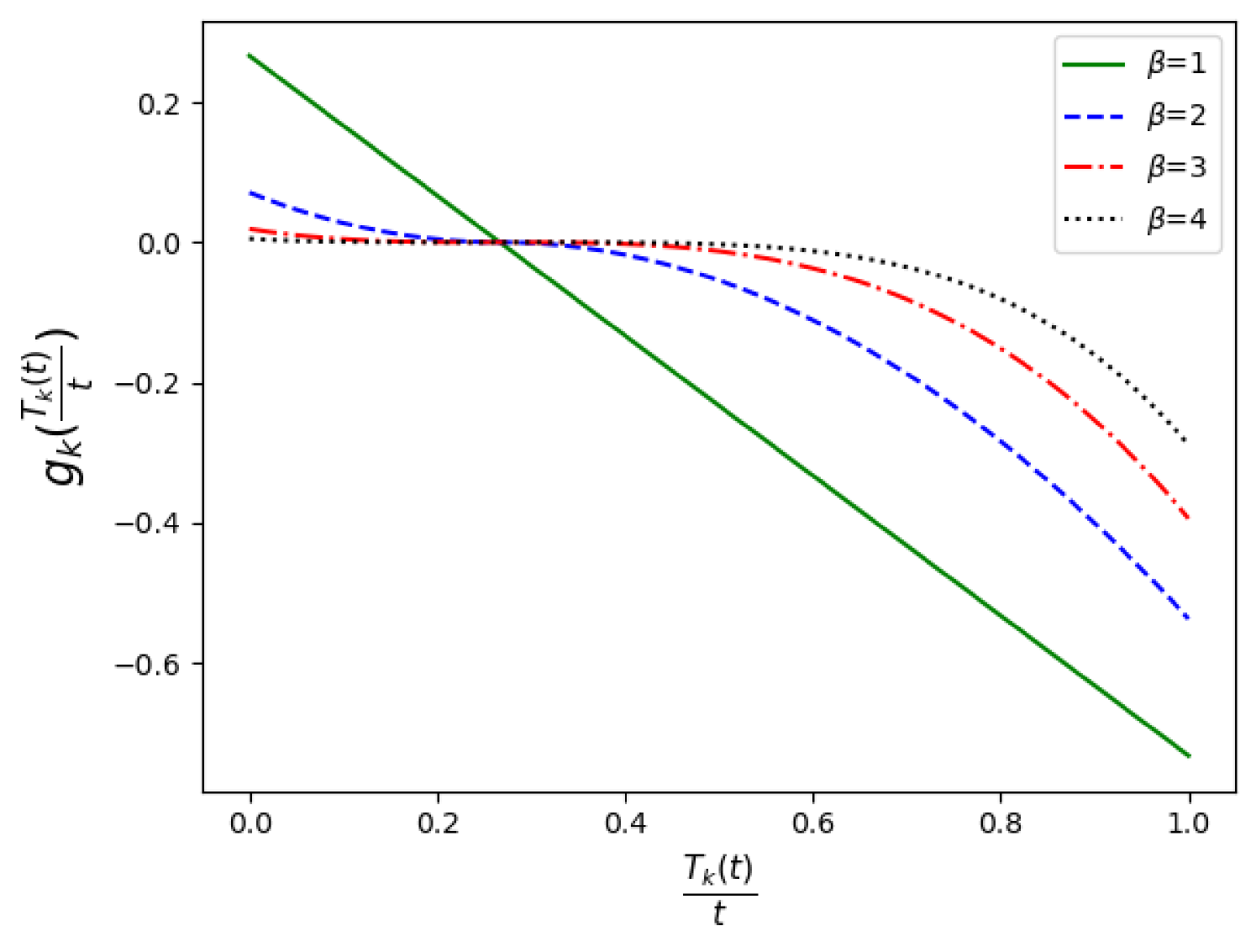
The second term is the generalization reward, designed to meet C1. It assigns higher values for users whose data have been underutilized compared to the relative size of their data from the whole available data, $\frac{|\mathcal{D}_{k}|}{|\mathcal{D}|}$. We adopt the generalization reward proposed in [23], which was shown to account for both i.i.d. balanced data and non-i.i.d. imbalanced data cases, and rewards the $k$th user in an $m$-sized group at round $t$ via the function

In (8), $\beta>1$ is a hyper-parameter that adjusts the fuzziness of the function, i.e., higher $\beta$ yields lower absolute value where the other parameters are fixed. Fig. 1 describes $g_{k}(\cdot)$ as a function of ${T_{k}(t)}/{t}$, and illustrates the effect of different $\beta$ values as means of balancing the reward assigned to users that participated much (high ${T_{k}(t)}/{t}$).

Our proposed reward encompasses the above terms, grading the selection of a group of users $\mathcal{S}$ of size $m$ at round $t$ as

The reward in (9) is composed of three additive terms which correspond to C2, C1 and C3, respectively, with $\alpha$ and $\gamma$ being hyper-parameters balancing these considerations. At this point we can make two remarks regarding the reward (9):

1. 1.

   Both $g_{k}(\cdot)$ and $p_{k}(\cdot)$ penalize repeated selection of the same users. However, each rewards differently, based on generalization and privacy considerations. The former accounts for the relative dataset sizes of the users, while the latter doesn’t. In the case of homogeneous data, where for all $k\in\mathbb{K}$, $|\mathcal{D}_{k}|=\frac{|\mathcal{D}|}{K}$, both $g_{k}(\cdot)$ and $p_{k}(\cdot)$ play a similar role. However, they differ significantly in the non-i.i.d case.

2. 2.

   The value of the first term is determined solely by the slowest user. This non-linearity, combined with the two other terms, directs the algorithm we derive from this reward to select a group of users with similar latency in a given round.

Here, we present PAUSE, which is a combinatorical -based [42] algorithm based on the reward (9). To derive PAUSE, we seek a policy $\Pi\triangleq(\mathcal{S}_{1},\mathcal{S}_{2},...)$ such that $\mathbb{E}[\sum_{t=1}^{n}r(\mathcal{S}_{t},t)]$ is maximized over $n$. To maximize the given term, as is customary in MAB settings, we aim to minimize the regret, defined as the loss of the algorithm compared to an algorithm composed by a Genie that has prior knowledge of the expectations of the random variables, i.e., of $\mu_{k}\triangleq\mathbb{E}[\frac{\tau_{\min}}{\tau_{k}}]$.

We define the Genie’s algorithm as selecting

where

The Genie policy (10) attempts to maximize the expectation of the reward (9) in each round, by replacing the order of the expectation and the $\min_{k\in\mathcal{S}}$ operator. As the reward $C^{\mathcal{G}}$ is history-dependent, the Genie’s policy is history-dependent as well.

We use the Genie policy to derive PAUSE, denoted $\mathcal{P}\triangleq(\mathcal{P}_{1},\mathcal{P}_{2},\ldots)$, as an upper confidence bound (ucb)-type algorithm [41]. Accordingly, PAUSE estimates the unknown expectations $\{\mu_{k}\}$ with their empirical means, computed using the latency measured in previous rounds via

Note that (11) can be efficiently updated in a recursive manner, as

PAUSE uses (11) to compute the ucb terms for each user at the end of the $t$th round [41], via

The ucb term in (13) is designed to tackle C2. Its formulation encapsulates the inherent exploration vs. exploitation trade-off in MAB problems, boosting exploitation of the fastest users in expectation using $\overline{\mu_{k}}(t)$, while encouraging to explore other users in its second term. The resulting user selection rule at round $t$ is

The overall active user selection procedure is summarized as Algorithm 1. The chosen users send their noisy local model updates to the server which updates the global model by (2) and sends it back to all the users in $\mathbb{K}$. At the end of every round, we update the users’ reward terms for the next round, in which $p_{k}(t)$ and $\overline{\mu_{k}}(t)$ change their values only for participating users $k\in\mathcal{P}_{t}$. Note that, by the formulation of Algorithm 1, it holds that when $m$ is an integer divisor of $K$, then in the first $\frac{K}{m}$ rounds, the server chooses every user exactly once due to the initial conditions.

To evaluate PAUSE, we next analyze its regret, which for a policy $\Pi$ is defined as the expectation of the reward gap between the given policy and the Genie’s policy:

We define the maximal reward gap for any policy as $\Delta_{\max}\triangleq\max_{t\in\mathbb{N},\Pi}r(\mathcal{G}_{t},t)-r(\mathcal{S}_{t},t)$. This quantity is bounded as stated the following lemma:

We bound the regret of PAUSE in the following theorem:

Theorem 3 bounds the regret accumulated at every round $n$. In the asymptotic regime, it implies that PAUSE achieves a regret growth whose order does not exceed $\mathcal{O}(\log(n))$, being the best-known regret rate in MAB [41, 42].

PAUSE is particularly designed to facilitate privacy and communication constrained FL. It leverages MAB-based active user selection to dynamically cope with privacy leakage accumulation, without restricting the overall number of FL rounds as in [36, 20, 24]. PAUSE is theoretically shown to achieve best-known regret growth and it demonstrated promising results in our experiments as detailed in Section V.

The formulation of PAUSE in Algorithm 1 focuses on the server operation, requiring the users only to send their updates with the proper PPN. As such, it can be naturally combined with existing methods for alleviating latency and privacy via update encoding [4]. Moreover, the statement of Algorithm 1 complies with any privacy policy imposed, while adhering to the constraints C1-C3. This inherent adaptability makes it an agile solution across diverse policy frameworks.

A core challenge associated with applying PAUSE stems from the fact that (14) involves a brute search over $\binom{K}{m}$ options. Such computation is expected to become infeasible at large networks, i.e., as $K$ grows; making it incompatible with consideration C4. This complexity can be alleviated by approximating the brute search with low-complexity policies based on (14), as we do in the sequel.

To ease the computational efficiency of the search procedure in (14), we construct a graph structure where the set of vertices $\mathbb{V}$ comprises all possible subsets of $m$ users in $\mathbb{K}$. For each vertex (i.e., set of users) $\mathcal{V}\in\mathbb{V}$, we denote its neighboring set as $\mathcal{N}_{\mathcal{V}}$. Two vertices $\mathcal{V},\mathcal{U}\in\mathbb{V}$ are designated as neighbors, when they satisfy the following requirements:

1. R1

   The intersection of the vertices contains exactly $m-1$ elements, i.e., the sets of users $\mathcal{V}$ and $\mathcal{U}$ differ in a single user, thus $|\mathcal{V}\cap\mathcal{U}|=m-1$.

2. R2

   One of the users which appears in only a single set minimizes one of the terms of the selection rule (14) in its designated group. i.e., one of the sets is an active neighbor of the other. Mathematically, we say that $\mathcal{U}$ is an active neighbor of $\mathcal{V}$ (and $\mathcal{V}$ is a passive neighbor of $\mathcal{U}$) if the distinct node in $\mathcal{V}$, i.e., $k=\mathcal{V}\setminus\mathcal{U}$, holds

   	$\displaystyle k\in\Big{\{}$	$\displaystyle\operatorname*{arg\,min}\limits_{k^{\prime}\in\mathcal{V}}{\rm ucb}(k^{\prime},t-1),\operatorname*{arg\,min}\limits_{k^{\prime}\in\mathcal{V}}p_{k^{\prime}}(t-1),$
   		$\displaystyle\operatorname*{arg\,min}\limits_{k^{\prime}\in\mathcal{V}}g_{k^{\prime}}(t-1)\Big{\}}.$

The above graph construction is inherently undirected due to the symmetric nature of the neighbor relationships.

To formalize our optimization objective, we define the energy of each vertex as the quantity we seek to maximize in PAUSE’s search (14). Specifically, for any vertex $\mathcal{V}$, define

To identify a vertex exhibiting maximal energy, we introduce an optimized SA-based algorithm [43], which iteratively inspects vertices (i.e., candidate user sets) in the graph. The resulting procedure, detailed in Algorithm 2, is comprised of two stages taking place on FL round $t$: initilalziaiton and iterative search.

Initialization: Following established SA methodology, we maintain an auxiliary temperature sequence, whose $j$th entry is defined as $\tau_{j}=\frac{C}{\log(j+1)}$, where parameter $C>0$ exceeds the maximum energy differential between any pair of vertices in the graph. Thus, one must first set the value of $C$.

Accordingly, the initialization phase at round $t$ involves sorting all $K$ users according to their respective ${\rm ucb}(k,t-1)$, $p_{k}(t-1)$, and $g_{k}(t-1)$ values into three distinct lists. These three sorted lists are used first to determine an appropriate value for $C$. For each list $i\in{1,2,3}$, we denote $\mathcal{A}_{m}^{i}$ and $\mathcal{B}_{m}^{i}$ as the sets containing the $m$ users with minimal and maximal values, respectively. The parameter $C$ is then established as follows, where $\omega$ represents a small positive constant:

Iterative Search: The algorithm’s iterative phase updates an inspected vertex, moving at iteration $j$ from the previously inspected $\mathcal{V}_{j}$ into an updated $\mathcal{V}_{j+1}$. This necessitates the identification of $\mathcal{N}_{\mathcal{V}_{j}}$. We decompose this task into the discovery of active and passive neighbors as specified in R2, utilizing the previously constructed sorted lists:

1. N1

   Active Neighbor Identification - To determine the active neighbors in iteration $i$, we examine each sorted list (${\rm ucb}(k,t-1)$, $p_{k}(t-1)$, and $g_{k}(t-1)$) to identify the user with the minimal value within $\mathcal{V}_{j}$. An active neighbor is generated by substituting any of these minimal-value users with a user not present in $\mathcal{V}_{j}$. This procedure yields at most $3(K-m)$ active neighbors of $\mathcal{V}_{j}$.

2. N2

   Passive Neighbor Identification - For passive neighbors, we establish that a vertex $\mathcal{U}$ qualifies as a passive neighbor of $\mathcal{V}_{j}$ if it can be constructed through one of two mechanisms, illustrated using the ${\rm ucb}(k,t-1)$ sorted list. Let $a$ denote the user with minimal ${\rm ucb}(k,t-1)$ in $\mathcal{V}_{j}$ and $b$ represent the user with the second-minimal value. $\mathcal{U}$ is a passive neighbor of $\mathcal{V}_{j}$ if it is obtained by either:

   1. (a)

      Replace any user in $\mathcal{V}_{j}$ except $a$ with a user whose ${\rm ucb}(k,t-1)$ value is lower than $a$’s (positioned before $a$ in the sorted list).

   2. (b)

      Replace $a$ with a user whose ${\rm ucb}(k,t-1)$ value is lower than $b$’s (positioned before $b$ in the sorted list).

Once the neighbors set $\mathcal{N}_{\mathcal{V}_{j}}$ is formulated, the algorithm inspects a random neighbor $\mathcal{U}$. This set is inspected in the following iteration if it improves in terms of the energy (18) (for which it is also saved as the best set explored so far), or alternatively it is randomly selected with probability $\exp{\big{(}-\frac{E(\mathcal{U})-E(\mathcal{V}_{j})}{\tau_{j}}\big{)}}$. The resulting procedure is summarized as Algorithm 2.

The proposed SA-PAUSE implements its FL procedure with active user selection formulated, while using Algorithm 2 to approximate PAUSE’s search 14. SA-PAUSE thus realizes Algorithm 1 while replacing its Step 1 with Algorithm 2.

Optimality: The SA search of SA-PAUSE, detailed in Algorithm 2, replaces searching over all possible user selections with exploration over a graph. To show its validity, we first prove that it indeed finds the reward-maximizing set of users, as done in PAUSE. Since in general there may be more than one set of users that maximizes the reward (or equivalently, the energy (18)), we use $\mathcal{J}$ to denote the set of vertices exhibiting maximal energy in the graph. The ability of Algorithm 2 to recover the same users set as brute search via (14) (or one that is equivalent in terms of reward) is stated in the following theorem:

Theorem 4 shows that Algorithm 2 is guaranteed to recover the reward-maximizing users set in the horizon of infinite number of iterations. While the SA algorithm operates over a finite number of iterations, and Theorem 4 applies as $j\rightarrow\infty$, the carefully designed cooling temperature sequence and algorithmic structure ensure robust practical performance of SA algorithms [50, 51]. This efficacy is empirically validated in Section V.

Time-Complexity: Having shown that Algorithm 2 can approach the users set recovered via PAUSE, we next show that it satisfies its core motivation, i.e., carry out this computation with reduced complexity, and thus supports scalability. While inherently the number of selected users $m$ is smaller than the overall number of users $K$, and often $m\ll K$, we accommodate in our analysis computationally intensive settings where $m$ is allowed to grow with $K$, but in the order of $m=\Theta(K)$.

On each FL round $t$, the initialization phase requires $\mathcal{O}(K\log K)$ operations due to the list sorting procedures. During each iteration $j$, locating $\mathcal{V}_{j}$’s users’ indices in the sorted lists can be accomplished in $\mathcal{O}(K\log K)$ operations through pointer manipulation. The identification of $\mathcal{N}_{\mathcal{V}_{j}}$ exhibits complexity $\mathcal{O}(|\mathcal{N}_{\mathcal{V}_{j}}|)$, as each neighbor can be found in constant time. While the number of active neighbors is bounded by $3(K-m)$, the quantity of passive neighbors varies across users and iterations. Given that each passive neighbor of $\mathcal{V}_{j}$ corresponds to that node being an active neighbor of $\mathcal{V}_{j}$, and considering the bounded number of active neighbors per user, a balanced graph typically exhibits approximately $3(K-m)$ passive neighbors per user. Specifically, in the average case where each user in $\mathbb{V}$ has $\mathcal{O}(K\log K)$ passive neighbors, the complexity order of Algorithm 2 is $\mathcal{O}(K\log K)$.

For comparative purposes, consider a simplified SA variant (termed Vanilla-SA) where the neighboring criterion is reduced to only the first condition in R1 (i.e., nodes are neighbors if they share exactly $m-1$ users). This algorithm closely resembles Algorithm 2, but eliminates list sorting and determines $N_{\mathcal{V}_{j}}$ by exhaustively replacing each user in $\mathcal{V}_{j}$ with each user in $\mathbb{K}\setminus\{\mathcal{V}_{j}\}$. In this case, by setting $C$ to be an upper bound on $\Delta_{max}$ (16), e.g., $C\triangleq 2\alpha+\gamma+1$ we satisfy the conditions for Theorem 4 as well, ensuring asymptotic convergence. However, this approach results in $|N_{\mathcal{V}_{j}}|=m(K-m)$, producing a densely connected graph that impedes search efficiency and invariably yields $\mathcal{O}(K^{2})$ complexity. Table I presents a comprehensive comparison of time complexities across different scenarios.

Here, we numerically evaluate PAUSE in FL¹¹1The source code used in our experimental study, including all the hyper-parameters, is available online at https://github.com/oritalp/PAUSE/tree/production. We consider the training of a DNN for image classification based on MNIST and CIFAR-10. The trained model is comprised of a convolutional neural network (CNN) with three hidden layers. These layers are followed by a fully-connected network (FC) with two hidden layers for CIFAR-10, and a three-layer FC with 32 neurons at its widest layer for MNIST.

We examine our approach in both small and large network settings with varying privacy budgets. In the former, the data is divided between $K=30$ users, and $m=5$ of them being chosen at each round, while the latter corresponds to $K=300$ and $m=15$ users. The communication latency $\tau_{k}$ obeys a normal distribution for every $k\in\mathbb{K}$. The users are equally divided into two groups: fast users, who had lower communication latency expectations, and slower users. For each configuration, we test our approach both in i.i.d and non-i.i.d data distributions. In the imbalnaced case, the data quantities are sampled from a Dirichlet distribution with parameter $\bm{\alpha}$, where each user exhibits a dominant label comprising approximately a quarter of the data.

As PAUSE becomes computationally infeasible in the large network case, it is only tested on small networks, while SA-PAUSE is being tested in both scenarios. These algorithms are compared with the following benchmarks:

• •

  Random, uniformly sampling $m=5$ users without replacements [44], solely in the i.i.d balanced case.

• •

  FedAvg with privacy and FedAvg w.o. privacy, choosing all $K$ users, with and without privacy, respectively.

• •

  Fastest in expectation, using only the same pre-known five fastest $m$ users in expectation at each round.

• •

  The clustered sampling selection algorithm proposed in [20].

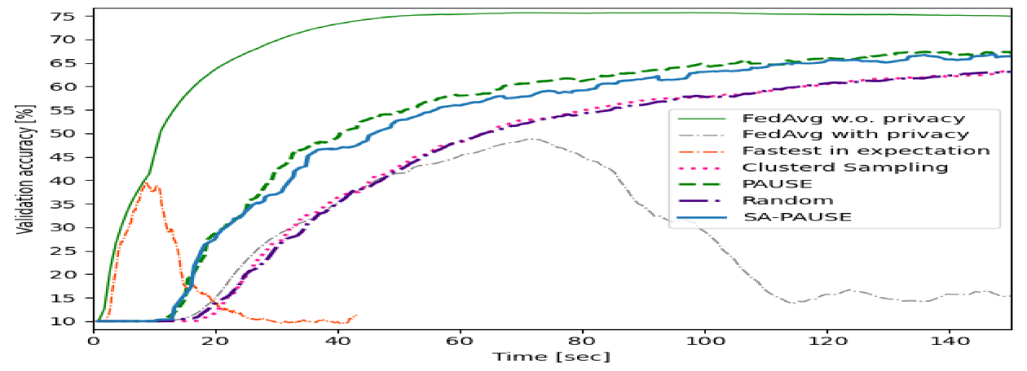
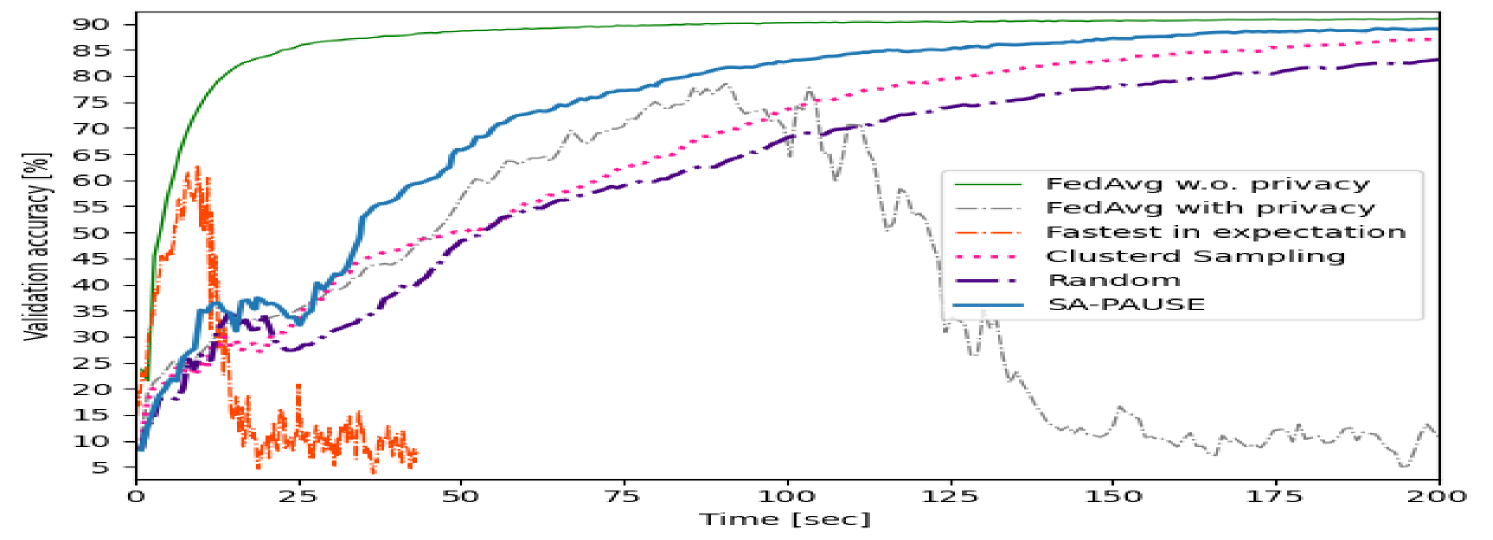
Our first study trains the mentioned CNN with an overall privacy budget of $\bar{\epsilon}=40$ for image classification using the CIFAR-10 dataset. The resulting FL accuracy versus communication latency are illustrated in Fig. 2. The error curves were smoothened with an averaging window of size $10$ to attenuate the fluctuations. As expected, due to privacy leakage accumulation, the more rounds a user participates in, the noisier its updates are. This is evident in Fig. 2, where choosing all users quickly results in ineffective updates. PAUSE consistently achieves both accurate learning and rapid convergence. Further observing this figure indicates SA-PAUSE successfully approximates PAUSE’s brute-force search as well.

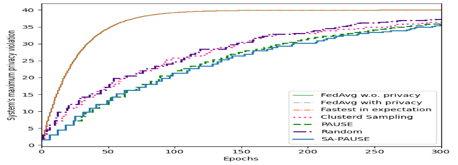
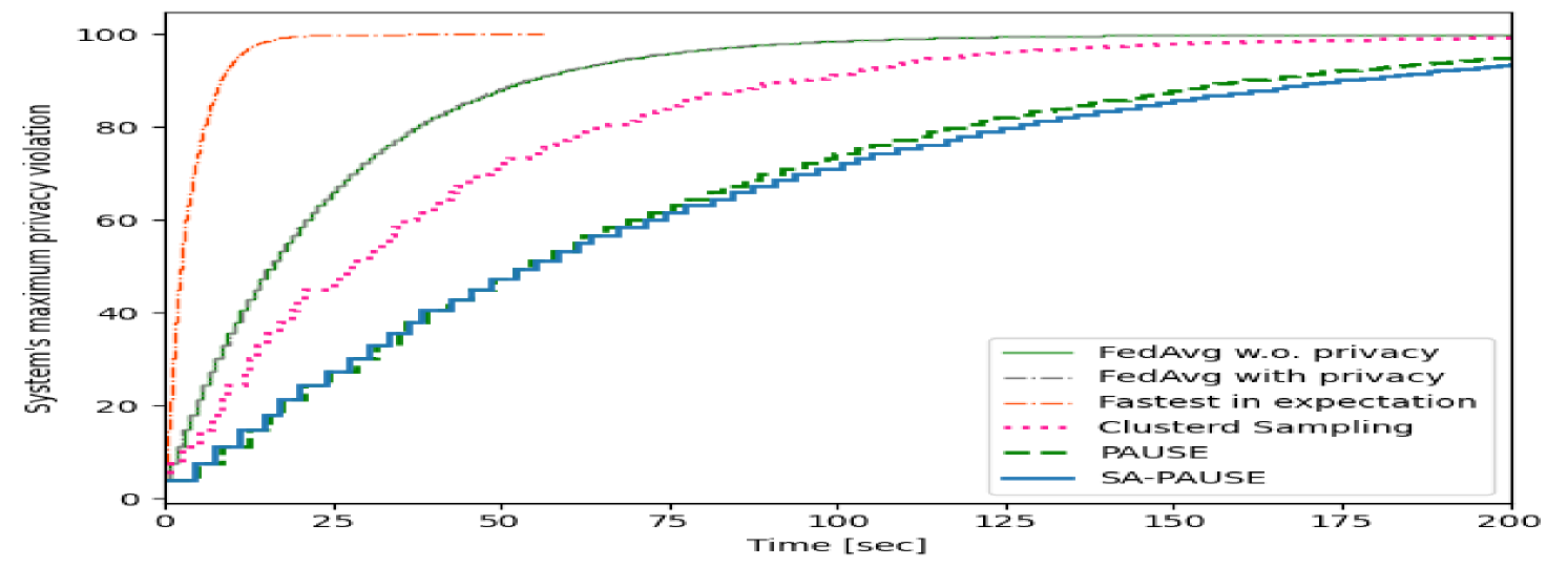
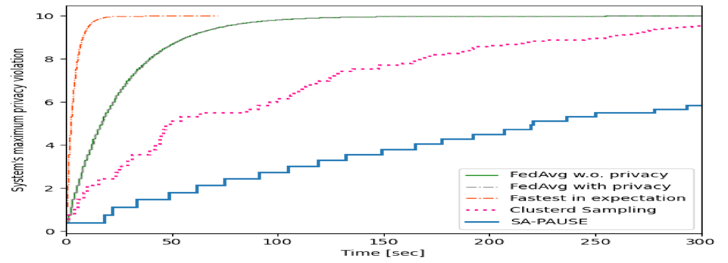
PAUSE’s ability to mitigate privacy accumulation is showcased in Fig. 3. There, we report the overall leakage as it evolves over epochs. Fig. 3 reveals that the privacy violation at each given epoch using PAUSE is lower compared to the random and the clustered sampling methods, adding to its improved accuracy and latency noted in Fig. 2. Note FedAvg with privacy and fastest in expectation methods’ maximum privacy violation coincide as in every epoch it’s raised by an $\epsilon_{i}$.

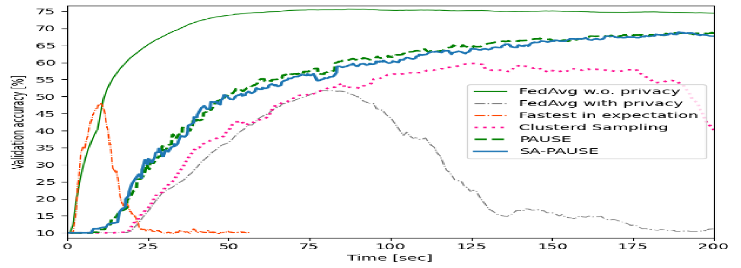
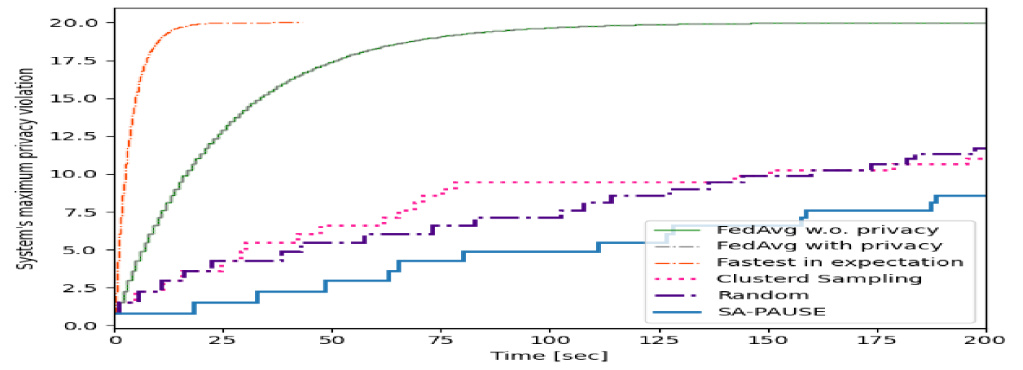
Subsequently, we train the same DNN with CIFAR-10 in the non-i.i.d case as described previously with an overall privacy budget of $\bar{\epsilon}=100$. As opposed to the balanced data test, this setting necessitates balancing between users with varying quantities of data, which might contribute differently to the learning process. The data quantities were sampled from a Dirichlet distribution with parameter ${\bm{\alpha}}={\bm{3}}$. Analyzing the validation accuracy versus communication latency in Fig. 4 indicates the superiority of our algorithms also in this case in terms of accuracy and latency. Fig. 5 depicts the maximum privacy violation of the system, this time, versus the communication latency, and facilitates this statement by demonstrating both PAUSE and its approximation’s ability to maintain privacy better though performing more sever-clients iterations in any given time.

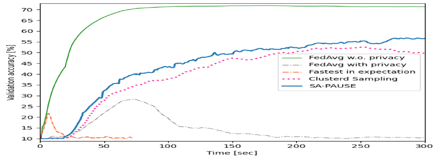
We proceed to consider the large network settings. Here, we train two models: one for MNIST with i.i.d. data distribution, and on for CIFAR-10 with data distributed non-i.i.d. For these scenarios, we implemented two modifications. First, to accelerate the convergence of the SA procedure in Algorithm 2 under a reasonable amount of iterations, we modulate the temperature coefficient $C$ as in  [52, 53]. This is accomplished by dividing the temperature coefficient by a constant $\kappa=30$, i.e., the temperature in the $j$th iteration becomes $\tau_{j}=\frac{C}{\kappa\log(1+j)}$ [52, 53]. Second, to enhance exploitation [54, 55], we amplified the empirical mean $\overline{\mu_{k}}(t)$ in 13 by another constant, $\zeta=3$.

The overall privacy budgets for the MNIST and CIFAR-10 evaluations are set to $\bar{\epsilon}=20$ and $\bar{\epsilon}=10$, respectively. In the former, the data quantities were sampled from a Dirichlet distribution with parameter ${\bm{\alpha}}={\bm{2}}$. Both cases exhibited consistent trends with the small networks tests, systematically demonstrating SA-PAUSE’s robustness across diverse privacy budgets, datasets, and network scales.

As before, the validation accuracy versus communication latency graphs are presented in Fig. 6 and Fig. 8, while the maximum overall privacy leakage versus time graphs are depicted in 7 and Fig. 9. These results systematically demonstrate the ability of our proposed SA-PAUSE to facilitate rapid learning over large networks with balanced and limited privacy leakage.

In the following, define $h_{k}(t)\triangleq\sqrt{\frac{(m+1)\log(t)}{T_{k}(t)}}$. The regret can be bounded following the definition of $\Delta_{max}$ as

We introduce another indicator function for every $i\in\mathbb{K}$ along with its cumulative sum, denoted:

Let $\mathcal{C}_{t}\triangleq\mathcal{P}_{t}\cup\mathcal{G}_{t}$. In every round $t$ where $r(\mathcal{P}_{t})\neq r(\mathcal{G}_{t})$, the counter $N_{k}(t)$ is incremented for only a single user in $\mathcal{C}_{t}$, while for the remaining users $N_{k}(t-1)=N_{k}(t)$. Thus, it holds that $\sum_{t=1}^{n}\mathbf{1}\big{(}(\mathcal{G}_{t},t)\neq r(\mathcal{P}_{t},t)\big{)}=\sum_{k=1}^{K}N_{k}(n)$. Substituting this into (-A.1), we obtain that

In the remainder, we focus on bounding $\mathbb{E}[N_{k}(n)]$ for every $k\in\mathbb{K}$. After that, we substitute the derived upper bound into (-A.2). To that aim, let $k\in\mathbb{K}$ and fix some $l\in\mathbb{N}$ whose value is determined later). We note that:

where $(a)$ arises from considering the cases $N_{k}(n)\leq l$ and its complementary state.

PAUSE’s policy (14) implies that in every iteration:

Since this happens with probability one, we can incorporate it into the mentioned inequality (-A.3):

We now denote the users chosen in the $t$th iteration by the PAUSE algorithm and by the Genie as: $\mathcal{G}_{t}=\tilde{u}_{t,1},...,\tilde{u}_{t,m}$ and $\mathcal{P}_{t}=u_{t,1},...,u_{t,m}$, respectively. For every $t$, the indicator function in the sum is equal to 1 only if the $k$th user is chosen the least at the beginning of the $t$th iteration, i.e., $T_{k}(t-1)\leq T_{j}(t-1)$ for every $j\in\mathcal{C}_{t}$. The intersection of $I_{k}(t)=1$ with $N_{k}(t)>l$ implies $T_{k}(t-1)\leq l$. Therefore, this intersection of events implies that for every $j\in\mathcal{C}_{t},l\leq T_{j}(t-1)\leq t-1$. Using this result, we can further bound every event in the indicator functions in the upper bound of $\mathbb{E}[N_{k}(n)]$:

Using the fact that for any finite set of events of size $q$, it holds that $\{A_{i}\}_{i=1}^{q}$, $\mathbf{1}(\cup_{i=1}^{q}A_{i})\leq\sum_{i=1}^{q}\mathbf{1}(A_{i})$, and that the expectation of an indicator function is the probability of the internal event occurring, we have that

In the following steps we focus on bounding the terms in the double sum. To that aim, we define the following:

Using these notations and writing $h_{a_{t}}\triangleq h_{a_{t}}(t)$, we state the following lemma:

References

- [1] O. Peleg, N. Lang, S. Rini, N. Shlezinger, and K. Cohen, “PAUSE: Privacy-aware active user selection for federated learning,” in IEEE International Conference on Acoustics, Speech and Signal Processing (ICASSP), 2025.
- [2] B. McMahan, E. Moore, D. Ramage, S. Hampson, and B. A. y Arcas, “Communication-efficient learning of deep networks from decentralized data,” in Artificial Intelligence and Statistics. PMLR, 2017, pp. 1273–1282.
- [3] P. Kairouz et al., “Advances and open problems in federated learning,” Foundations and trends® in machine learning, vol. 14, no. 1–2, pp. 1–210, 2021.
- [4] T. Gafni, N. Shlezinger, K. Cohen, Y. C. Eldar, and H. V. Poor, “Federated learning: A signal processing perspective,” IEEE Signal Process. Mag., vol. 39, no. 3, pp. 14–41, 2022.
- [5] T. Li, A. K. Sahu, A. Talwalkar, and V. Smith, “Federated learning: Challenges, methods, and future directions,” IEEE Signal Process. Mag., vol. 37, no. 3, pp. 50–60, 2020.
- [6] M. Chen, N. Shlezinger, H. V. Poor, Y. C. Eldar, and S. Cui, “Communication-efficient federated learning,” Proceedings of the National Academy of Sciences, vol. 118, no. 17, 2021.
- [7] D. Alistarh, T. Hoefler, M. Johansson, N. Konstantinov, S. Khirirat, and C. Renggli, “The convergence of sparsified gradient methods,” Advances in Neural Information Processing Systems, vol. 31, 2018.
- [8] P. Han, S. Wang, and K. K. Leung, “Adaptive gradient sparsification for efficient federated learning: An online learning approach,” in IEEE International Conference on Distributed Computing Systems (ICDCS), 2020, pp. 300–310.
- [9] A. Reisizadeh, A. Mokhtari, H. Hassani, A. Jadbabaie, and R. Pedarsani, “Fedpaq: A communication-efficient federated learning method with periodic averaging and quantization,” in International Conference on Artificial Intelligence and Statistics. PMLR, 2020, pp. 2021–2031.
- [10] N. Shlezinger, M. Chen, Y. C. Eldar, H. V. Poor, and S. Cui, “UVeQFed: Universal vector quantization for federated learning,” IEEE Trans. Signal Process., vol. 69, pp. 500–514, 2020.
- [11] M. M. Amiri and D. Gündüz, “Machine learning at the wireless edge: Distributed stochastic gradient descent over-the-air,” IEEE Trans. Signal Process., vol. 68, pp. 2155–2169, 2020.
- [12] T. Sery and K. Cohen, “On analog gradient descent learning over multiple access fading channels,” IEEE Trans. Signal Process., vol. 68, pp. 2897–2911, 2020.
- [13] K. Yang, T. Jiang, Y. Shi, and Z. Ding, “Federated learning via over-the-air computation,” IEEE Trans. Wireless Commun., vol. 19, no. 3, pp. 2022–2035, 2020.
- [14] S. Mayhoub and T. M. Shami, “A review of client selection methods in federated learning,” Archives of Computational Methods in Engineering, vol. 31, no. 2, pp. 1129–1152, 2024.
- [15] J. Li, T. Chen, and S. Teng, “A comprehensive survey on client selection strategies in federated learning,” Computer Networks, p. 110663, 2024.
- [16] L. Fu, H. Zhang, G. Gao, M. Zhang, and X. Liu, “Client selection in federated learning: Principles, challenges, and opportunities,” IEEE Internet Things J., vol. 10, no. 24, pp. 21 811–21 819, 2023.
- [17] J. Xu and H. Wang, “Client selection and bandwidth allocation in wireless federated learning networks: A long-term perspective,” IEEE Trans. Wireless Commun., vol. 20, no. 2, pp. 1188–1200, 2020.
- [18] S. AbdulRahman, H. Tout, A. Mourad, and C. Talhi, “FedMCCS: Multicriteria client selection model for optimal iot federated learning,” IEEE Internet Things J., vol. 8, no. 6, pp. 4723–4735, 2020.
- [19] E. Rizk, S. Vlaski, and A. H. Sayed, “Federated learning under importance sampling,” IEEE Trans. Signal Process., vol. 70, pp. 5381–5396, 2022.
- [20] Y. Fraboni, R. Vidal, L. Kameni, and M. Lorenzi, “Clustered sampling: Low-variance and improved representativity for clients selection in federated learning,” in International Conference on Machine Learning. PMLR, 2021, pp. 3407–3416.
- [21] W. Xia, T. Q. Quek, K. Guo, W. Wen, H. H. Yang, and H. Zhu, “Multi-armed bandit-based client scheduling for federated learning,” IEEE Trans. Wireless Commun., vol. 19, no. 11, pp. 7108–7123, 2020.
- [22] B. Xu, W. Xia, J. Zhang, T. Q. Quek, and H. Zhu, “Online client scheduling for fast federated learning,” IEEE Wireless Commun. Lett., vol. 10, no. 7, pp. 1434–1438, 2021.
- [23] D. Ben-Ami, K. Cohen, and Q. Zhao, “Client selection for generalization in accelerated federated learning: A multi-armed bandit approach,” IEEE Access, 2025.
- [24] Y. Chen, W. Xu, X. Wu, M. Zhang, and B. Luo, “Personalized local differentially private federated learning with adaptive client sampling,” in IEEE International Conference on Acoustics, Speech and Signal Processing (ICASSP), 2024, pp. 6600–6604.
- [25] L. Zhu and S. Han, “Deep leakage from gradients,” in Federated learning. Springer, 2020, pp. 17–31.
- [26] B. Zhao, K. R. Mopuri, and H. Bilen, “iDLG: Improved deep leakage from gradients,” arXiv preprint arXiv:2001.02610, 2020.
- [27] Y. Huang, S. Gupta, Z. Song, K. Li, and S. Arora, “Evaluating gradient inversion attacks and defenses in federated learning,” Advances in Neural Information Processing Systems, vol. 34, 2021.
- [28] H. Yin, A. Mallya, A. Vahdat, J. M. Alvarez, J. Kautz, and P. Molchanov, “See through gradients: Image batch recovery via gradinversion,” in Proceedings of the IEEE/CVF Conference on Computer Vision and Pattern Recognition, 2021, pp. 16 337–16 346.
- [29] M. Kim, O. Günlü, and R. F. Schaefer, “Federated learning with local differential privacy: Trade-offs between privacy, utility, and communication,” in IEEE International Conference on Acoustics, Speech and Signal Processing (ICASSP), 2021, pp. 2650–2654.
- [30] K. Wei et al., “Federated learning with differential privacy: Algorithms and performance analysis,” IEEE Trans. Inf. Forensics Security, vol. 15, pp. 3454–3469, 2020.
- [31] L. Lyu, “DP-SIGNSGD: When efficiency meets privacy and robustness,” in IEEE International Conference on Acoustics, Speech and Signal Processing (ICASSP), 2021, pp. 3070–3074.
- [32] A. Lowy and M. Razaviyayn, “Private federated learning without a trusted server: Optimal algorithms for convex losses,” in International Conference on Learning Representations, 2023.
- [33] N. Lang, E. Sofer, T. Shaked, and N. Shlezinger, “Joint privacy enhancement and quantization in federated learning,” IEEE Trans. Signal Process., vol. 71, pp. 295–310, 2023.
- [34] N. Lang, N. Shlezinger, R. G. D’Oliveira, and S. E. Rouayheb, “Compressed private aggregation for scalable and robust federated learning over massive networks,” arXiv preprint arXiv:2308.00540, 2023.
- [35] C. Dwork, G. N. Rothblum, and S. Vadhan, “Boosting and differential privacy,” in IEEE Annual Symposium on Foundations of Computer Science, 2010, pp. 51–60.
- [36] J. Zhang, D. Fay, and M. Johansson, “Dynamic privacy allocation for locally differentially private federated learning with composite objectives,” in IEEE International Conference on Acoustics, Speech and Signal Processing (ICASSP), 2024, pp. 9461–9465.
- [37] L. Sun, J. Qian, X. Chen, and P. S. Yu, “LDP-FL: Practical private aggregation in federated learning with local differential privacy,” in International Joint Conference on Artificial Intelligence, 2021.
- [38] A. Cheu, A. Smith, J. Ullman, D. Zeber, and M. Zhilyaev, “Distributed differential privacy via shuffling,” in Advances in Cryptology–EUROCRYPT 2019: 38th Annual International Conference on the Theory and Applications of Cryptographic Techniques, Darmstadt, Germany, May 19–23, 2019, Proceedings, Part I 38. Springer, 2019, pp. 375–403.
- [39] B. Balle, J. Bell, A. Gascón, and K. Nissim, “The privacy blanket of the shuffle model,” in Advances in Cryptology–CRYPTO 2019: 39th Annual International Cryptology Conference, Santa Barbara, CA, USA, August 18–22, 2019, Proceedings, Part II 39. Springer, 2019, pp. 638–667.
- [40] Q. Zhao, Multi-armed bandits: Theory and applications to online learning in networks. Springer Nature, 2022.
- [41] P. Auer, N. Cesa-Bianchi, and P. Fischer, “Finite-time analysis of the multiarmed bandit problem,” Machine learning, vol. 47, pp. 235–256, 2002.
- [42] W. Chen, Y. Wang, and Y. Yuan, “Combinatorial multi-armed bandit: General framework and applications,” in International conference on machine learning. PMLR, 2013, pp. 151–159.
- [43] B. Hajek, “Cooling schedules for optimal annealing,” Mathematics of operations research, vol. 13, no. 2, pp. 311–329, 1988.
- [44] X. Li, K. Huang, W. Yang, S. Wang, and Z. Zhang, “On the convergence of FedAvg on non-iid data,” in International Conference on Learning Representations, 2019.
- [45] N. Lang, A. Cohen, and N. Shlezinger, “Stragglers-aware low-latency synchronous federated learning via layer-wise model updates,” IEEE Trans. on Commun., 2024, early access.
- [46] S. P. Kasiviswanathan, H. K. Lee, K. Nissim, S. Raskhodnikova, and A. Smith, “What can we learn privately?” SIAM Journal on Computing, vol. 40, no. 3, pp. 793–826, 2011.
- [47] Y. Wang, Y. Tong, and D. Shi, “Federated latent dirichlet allocation: A local differential privacy based framework,” in Proceedings of the AAAI Conference on Artificial Intelligence, vol. 34, no. 04, 2020, pp. 6283–6290.
- [48] T. Wang, X. Zhang, J. Feng, and X. Yang, “A comprehensive survey on local differential privacy toward data statistics and analysis,” Sensors, vol. 20, no. 24, p. 7030, 2020.
- [49] C. Dwork, F. McSherry, K. Nissim, and A. Smith, “Calibrating noise to sensitivity in private data analysis,” Journal of Privacy and Confidentiality, vol. 7, no. 3, pp. 17–51, 2016.
- [50] D. Henderson, S. H. Jacobson, and A. W. Johnson, “The theory and practice of simulated annealing,” Handbook of metaheuristics, pp. 287–319, 2003.
- [51] S. Ledesma, G. Aviña, and R. Sanchez, “Practical considerations for simulated annealing implementation,” Simulated annealing, vol. 20, pp. 401–420, 2008.
- [52] W. Ben-Ameur, “Computing the initial temperature of simulated annealing,” Computational optimization and applications, vol. 29, pp. 369–385, 2004.
- [53] I. Bezáková, D. Štefankovič, V. V. Vazirani, and E. Vigoda, “Accelerating simulated annealing for the permanent and combinatorial counting problems,” SIAM Journal on Computing, vol. 37, no. 5, pp. 1429–1454, 2008.
- [54] H. Wu, X. Guo, and X. Liu, “Adaptive exploration-exploitation tradeoff for opportunistic bandits,” in International Conference on Machine Learning. PMLR, 2018, pp. 5306–5314.
- [55] M. M. Drugan, A. Nowé, and B. Manderick, “Pareto upper confidence bounds algorithms: an empirical study,” in IEEE Symposium on Adaptive Dynamic Programming and Reinforcement Learning (ADPRL), 2014.
- [56] W. Hoeffding, “Probability inequalities for sums of bounded random variables,” The collected works of Wassily Hoeffding, pp. 409–426, 1994.