PDE-Net 2.0: Learning PDEs from Data with A Numeric-Symbolic Hybrid Deep Network
Abstract
Partial differential equations (PDEs) are commonly derived based on empirical observations. However, recent advances of technology enable us to collect and store massive amount of data, which offers new opportunities for data-driven discovery of PDEs. In this paper, we propose a new deep neural network, called PDE-Net 2.0, to discover (time-dependent) PDEs from observed dynamic data with minor prior knowledge on the underlying mechanism that drives the dynamics. The design of PDE-Net 2.0 is based on our earlier work [1] where the original version of PDE-Net was proposed. PDE-Net 2.0 is a combination of numerical approximation of differential operators by convolutions and a symbolic multi-layer neural network for model recovery. Comparing with existing approaches, PDE-Net 2.0 has the most flexibility and expressive power by learning both differential operators and the nonlinear response function of the underlying PDE model. Numerical experiments show that the PDE-Net 2.0 has the potential to uncover the hidden PDE of the observed dynamics, and predict the dynamical behavior for a relatively long time, even in a noisy environment.
Keywords Partial differential equations dynamic system convolutional neural network symbolic neural network
1 Introduction
Differential equations, especially partial differential equations(PDEs), play a prominent role in many disciplines to describe the governing physical laws underlying a given system of interest. Traditionally, PDEs are derived mathematically or physically based on some basic principles, e.g. from Schrödinger’s equations in quantum mechanics to molecular dynamic models, from Boltzmann equations to Navier-Stokes equations, etc. However, the mechanisms behind many complex systems in modern applications (such as many problems in multiphase flow, neuroscience, finance, biological science, etc.) are still generally unclear, and the governing equations of these systems are commonly obtained by empirical formulas [2, 3]. With the recent rapid development of sensors, computational power, and data storage in the last decade, huge quantities of data can now be easily collected, stored and processed. Such vast quantity of data offers new opportunities for data-driven discovery of (potentially new) physical laws. Then, one may ask the following interesting and intriguing question: can we learn a PDE model to approximate the observed complex dynamic data?
1.1 Existing Work and Motivations
Earlier attempts on data-driven discovery of hidden physical laws include [4, 5]. Their main idea is to compare numerical differentiations of the experimental data with analytic derivatives of candidate functions, and apply the symbolic regression and the evolutionary algorithm to determining the nonlinear dynamic system. When the form of the nonlinear response function of a PDE is known, except for some scalar parameters, [6] presented a framework to learn these unknown parameters by introducing regularity between two consecutive time step using Gaussian process. Later in [7], a PDE constraint interpolation method was introduced to uncover the unknown parameters of the PDE model. An alternative approach is known as the sparse identification of nonlinear dynamics (SINDy) [8, 9, 10, 11, 12, 13]. The key idea of SINDy is to first construct a dictionary of simple functions and partial derivatives that are likely to appear in the equations. Then, it takes the advantage of sparsity promoting techniques (e.g. regularization) to select candidates that most accurately represent the data. In [14], the authors studied the problem of sea surface temperature prediction (SSTP). They assumed that the underlying physical model was an advection-diffusion equation. They designed a special neural network according to the general solution of the equation. Comparing with traditional numerical methods, their approach showed improvements in accuracy and computation efficiency.
Recent work greatly advanced the progress of PDE identification from observed data. However, SINDy requires to build a sufficiently large dictionary which may lead to high memory load and computation cost, especially when the number of model variables is large. Furthermore, the existing methods based on SINDy treat spatial and temporal information of the data separately and does not take full advantage of the temporal dependence of the PDE model. Although the framework presented by [6, 7] is able to learn hidden physical laws using less data than the approach based on SINDy, the explicit form of the PDEs is assumed to be known except for a few scalar learnable parameters. The approach of [14] is specifically designed for advection-diffusion equations, and cannot be readily extended to other types of equations. Therefore, extracting governing equations from data in a less restrictive setting remains a great challenge.
The main objective of this paper is to design a transparent deep neural network to uncover hidden PDE models from observed complex dynamic data with minor prior knowledge on the mechanisms of the dynamics, and to perform accurate predictions at the same time. The reason we emphasize on both model recovery and prediction is because: 1) the ability to conduct accurate long-term prediction is an important indicator of accuracy of the learned PDE model (the more accurate is the prediction, the more confident we have on the underlying recovered PDE model); 2) the trained neural network can be readily used in applications and does not need to be re-trained when initial conditions are altered. Our inspiration comes from the latest development of deep learning techniques in computer vision. An interesting fact is that some popular networks in computer vision, such as ResNet[15, 16], have close relationship with ODEs/PDEs and can be naturally merged with traditional computational mathematics in various tasks [17, 18, 19, 20, 21, 22, 23, 24, 25, 26]. However, existing deep networks designed in deep learning mostly emphasis on expressive power and prediction accuracy. These networks are not transparent enough to be able to reveal the underlying PDE models, although they may perfectly fit the observed data and perform accurate predictions. Therefore, we need to carefully design the network by combining knowledge from deep learning and numerical PDEs.
1.2 Our Approach
The proposed deep neural network is an upgraded version of our original PDE-Net [1]. The main difference is the use of a symbolic network to approximate the nonlinear response function, which significantly relaxes the requirement on the prior knowledge on the PDEs to be recovered. During training, we no longer need to assume the general type of the PDE (e.g. convection, diffusion, etc.) is known. Furthermore, due to the lack of prior knowledge on the general type of the unknown PDE models, more carefully designed constraints on the convolution filters as well as the parameters of the symbolic network are introduced. We refer to this upgraded network as PDE-Net 2.0.
Assume that the PDE to be recovered takes the following generic form
PDE-Net 2.0 is designed as a feed-forward network by discretizing the above PDE using forward Euler in time and finite difference in space. The forward Euler approximation of temporal derivative makes PDE-Net 2.0 ResNet-like [15, 18, 21], and the finite difference is realized by convolutions with trainable kernels (or filters). The nonlinear response function is approximated by a symbolic neural network, which shall be referred to as . All the parameters of the and the convolution kernels are jointly learned from data. To grant full transparency to the PDE-Net 2.0, proper constraints are enforced on the and the filters. Full details on the architecture and constraints will be presented in Section 2.
1.3 Relation with Model Reduction
Data-driven discovery of hidden physical laws and model reduction have a lot in common. Both of them concern on representing observed data using relatively simple models. The main difference is that, model reduction emphasis more on numerical precision rather than acquiring the analytic form of the model.
It is common practice in model reduction to use a function approximator to express the unknown terms in the reduced models, such as approximating subgrid stress for large-eddy simulation[27, 28, 29] or approximating interatomic forces for coarse-grained molecular dynamic systems[30, 31]. Our work may serve as an alternative approach to model reduction and help with analyzing the reduced models.
1.4 Novelty
The particular novelties of our approach are that we impose appropriate constraints on the learnable filters and use a properly designed symbolic neural network to approximate the response function . Using learnable filters makes the PDE-Net 2.0 more flexible, and enables more powerful approximation of unknown dynamics and longer time prediction (see numerical experiments in Section 3 and Section 4). Furthermore, the constraints on the learnable filters and the use of a deep symbolic neural network enable us to uncover the analytic form of with minor prior knowledge on the dynamic, which is the main advantage of PDE-Net 2.0 over the original PDE-Net. In addition, the composite representation by the symbolic network is more efficient and flexible than SINDy. Therefore, the proposed PDE-Net 2.0 is distinct from the existing learning based methods to discover PDEs from data.
2 PDE-Net 2.0: Architecture, Constraints and Training
Given a series of measurements of some physical quantities with being the number of physical quantities of interest, we want to discover the governing PDEs from the observed data . We assume that the observed data are associated with a PDE that takes the following general form:
| (1) |
here , , , . Our objective is to design a feed-forward network, called PDE-Net 2.0, to approximate the unknown PDE (1) from its solution samples in the way that: 1) we are able to reveal the analytic form of the response function and the differential operators involved; 2) we can conduct long-term prediction on the dynamical behavior of the equation for any given initial conditions. There are two main components of the PDE-Net 2.0 that are combined together in the same network: one is automatic determination on the differential operators involved in the PDE and their discrete approximations; the other is to approximate the nonlinear response function . In this section, we start with discussions on the overall framework of the PDE-Net 2.0 and then introduce the details on these two components. Regularization and training strategies will be given near the end of this section.
2.1 Architecture of PDE-Net 2.0
Inspired by the dynamic system perspective of deep neural networks [17, 18, 19, 20, 21, 22], we consider forward Euler as the temporal discretization of the evolution PDE (1), and unroll the discrete dynamics to a feed-forward network. One may consider more sophisticated temporal discretization which naturally leads to different network architectures [21]. For simplicity, we focus on forward Euler in this paper.
2.1.1 -block:
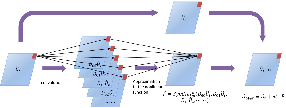
Let be the predicted value at time based on . Then, we design an approximation framework as follows
| (2) |
Here, the operators are convolution operators with the underlying filters denoted by , i.e. . The operators , , , etc. approximate differential operators, i.e. . In particular, the operators is a certain averaging operator. The purpose of introducing the average operators in stead of simply using the identity is to improve the expressive power of the network and enables it to capture more complex dynamics.
Other than the assumption that the observed dynamics is governed by a PDE of the form (1), we assume that the highest order of the PDE is less than some positive integer. Then, we can assume that is a function of variables with known . The task of approximating in (1) is equivalent to a multivariate regression problem. In order to be able to identify the analytic form of , we use a symbolic neural network denote by to approximate , where denotes the depth of the network. Note that, if is a vector function, we use multiple to approximate the components of separately.
Combining the aforementioned approximation of differential operators and the nonlinear response function, we obtain an approximation framework (2) which will be referred to as a -block (see Figure 1). Details of these two components can be found later in Section 2.2 and Section 2.3.
2.1.2 Multiple -Blocks:
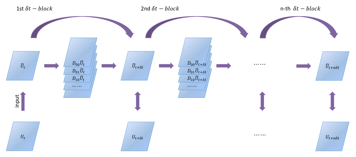
One -block only guarantees the accuracy of one-step dynamics, which does not take error accumulation into consideration. In order to facilitate a long-term prediction, we stack multiple -blocks into a deep network, and call this network the PDE-Net 2.0 (see Figure 2). The importance of stacking multiple -blocks will be demonstrated by our numerical experiments in Section 3 and 4.
The PDE-Net 2.0 can be easily described as: (1) stacking one -block multiple times; (2) sharing parameters in all -blocks. Given a set of observed data , training a PDE-Net 2.0 with -blocks needs to minimize the accumulated error , where is the output from the PDE-Net 2.0 (i.e. -blocks) with input , and is observed training data.
2.2 Convolutions and Differentiations
In the original PDE-Net [1], the learnable filters are properly constrained so that we can easily identify their correspondence to differential operators. PDE-Net 2.0 adopts the same constrains as the original version of the PDE-Net. For completeness, we shall review the related notions and concepts, and provide more details.
A profound relationship between convolutions and differentiations was presented by [32, 33], where the authors discussed the connection between the order of sum rules of filters and the orders of differential operators. Note that the definition of convolution we use follows the convention of deep learning, which is defined as
This is essentially correlation instead of convolution in the mathematics convention. Note that if is of finite size, we use periodic boundary condition.
The order of sum rules is closely related to the order of vanishing moments in wavelet theory [34, 35]. We first recall the definition of the order of sum rules.
Definition 2.1 (Order of Sum Rules)
For a filter , we say to have sum rules of order , where , provided that
| (3) |
for all with and for all with but . If (3) holds for all with except for with certain and , then we say to have total sum rules of order .
In practical implementation, the filters are normally finite and can be understood as matrices. For an filter ( being an odd number), assuming the indices of start from , (3) can be written in the following simpler form
The following proposition from [33] links the orders of sum rules with orders of differential operators.
Proposition 2.1
Let be a filter with sum rules of order . Then for a smooth function on , we have
| (4) |
If, in addition, has total sum rules of order for some , then
| (5) |
According to Proposition 2.1, an th order differential operator can be approximated by the convolution of a filter with order of sum rules. Furthermore, according to (5), one can obtain a high order approximation of a given differential operator if the corresponding filter has an order of total sum rules with . For example, consider filter
It has a sum rules of order , and a total sum rules of order . Thus, up to a constant and a proper scaling, corresponds to a discretization of with second order accuracy.
For an filter , define the moment matrix of as
| (6) |
where
| (7) |
We shall call the -element of the -moment of for simplicity. For any smooth function , we apply convolution on the sampled version of with respect to the filter . By Taylor’s expansion, one can easily obtain the following formula
| (8) | |||||
From (8) we can see that filter can be designed to approximate any differential operator with prescribed order of accuracy by imposing constraints on .
For example, if we want to approximate (up to a constant) by convolution where is a filter, we can consider the following constrains on :
| (9) |
Here, means no constraint on the corresponding entry. The constraints described by the moment matrix on the left of (9) guarantee the approximation accuracy is at least first order, and the one on the right guarantees an approximation of at least second order. In particular, when all entries of are constrained, e.g.
the corresponding filter can be uniquely determined. In the PDE-Net 2.0, all filters are learned subjected to partial constraints on their associated moment matrices, with at least second order accuracy.
2.3 Design of : a Symbolic Neural Network
The symbolic neural network of the PDE-Net 2.0 is introduced to approximate the multivariate nonlinear response function of (1). Neural networks have recently been proven effective in approximating multivariate functions in various scenarios [36, 37, 38, 39, 40]. For the problem we have in hand, we not only require the network to have good expressive power, but also good transparency so that the analytic form of can be readily inferred after training. Our design of is motivated by EQL/EQL÷ proposed by [41, 42].
The , as illustrated in Figure 3, is a network that takes an dimensional vector as input and has hidden layers.
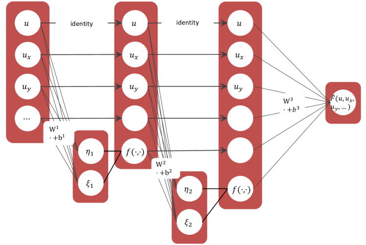
Figure 3 shows the symbolic neural network with two hidden layers, i.e. , where is a dyadic operation unit, e.g. multiplication or division. In this paper, we focus on multiplication, i.e. we take . Different from EQL/EQL÷, each hidden layer of the directly takes the outputs from the preceding layer as inputs, rather than a linear combination of them. Furthermore, it adds one additional variable (i.e. ) at each hidden layer. To better understand , we present an example in Algorithm 1 showing how is constructed. In particular, when ,
and , then which is the right-hand-side of of the Burgers’ equation without viscosity.
Input: ,
Output: .
The can represent all polynomials of variables with the total number of multiplications not exceeding . If needed, one can add more operations to the to increase the capacity of the network.
Now, we show that is more compact than the dictionaries of SINDy. For that, we first introduce some notions.
Definition 2.2
Define the set of all polynomials of variables with the total number of multiplications not exceeding as . Here, the total number of multiplications of is counted as follows:
-
•
For any monomial of degree , if , then the number of multiplications of the monomial is counted as . When or , the count is 0.
-
•
For any polynomial , the total number of multiplications is counted as the sum of the number of multiplications of its monomials.
For example, and with are all members of . The elements in are of simple forms when is relatively small. The following proposition shows that can represent all polynomials of variables with the total number of multiplications not exceeding . Note that the actual capacity of is larger than , i.e. is a subset of the set of functions that can represent.
Proposition 2.2
For any , there exists a set of parameters for such that
Proof: We prove this proposition by induction. When , the conclusion obviously holds. Suppose the conclusion holds for . For any polynomial , we only need to consider the cases when has a total number of multiplications greater than 1.
We take any monomial of that has degree greater than 1, which we suppose take the form where is a monomial of variable . Then, can be written as . Define new variable . Then, we have
By the induction hypothesis, there exists a set of parameters such that .
We take the linear transform between the input layer and the first hidden layer of as
Then, the output of the first hidden layer is . If we use it as the input of , we have
which concludes the proof.
SINDy constructs a dictionary that incudes all possible monomials up to a certain degree. Observe that there are totally monomials with variables and a degree not exceeding . Our symbolic network, however, is more compact than SINDy. The following proposition compares the complexity of and SINDy, whose proof is straightforward.
Proposition 2.3
Let and suppose have monomials of degree .
-
•
The memory load of that approximates is . The number of flops for evaluating is .
-
•
Constructing a dictionary with all possible polynomials of degree requires a memory load of , and evaluation of a linear combination of dictionary members requires flops.
We use the following example to show the advantage of over SINDy. Consider two variables and all of their derivatives of order :
Suppose the polynomial to be approximated is . For , the size of the dictionary of SINDy is and the computation of linear combination of the elements requires flops. The memory load of , however, is 15 and an evaluation of the network requires 180 flops. Therefore, can significantly reduce memory load and computation cost when input data is large. Note that when is large and small, is worse than SINDy. However, for system identification problems, we normally wish to obtain a compact representation (i.e. smaller ). Thus, takes full advantage of this prior knowledge and can significantly save on memory and computation cost which is crucial in the training of the PDE-Net 2.0.
2.4 Loss Function and Regularization
We adopt the following loss function to train the proposed PDE-Net 2.0:
where the hyper-parameters and are chosen as and . Now, we present details on each of the term of the loss function and introduce pseudo-upwind as an additional constraint on PDE-Net 2.0.
2.4.1 Data Approximation
Consider the data set , where is the number of -blocks and is the total number of samples. The index indicates the -th solution path with a certain initial condition of the unknown dynamics. Note that one can split a long solution path into multiple shorter ones. We would like to train the PDE-Net 2.0 with -blocks. For a given , every pair of the data , for each and , is a training sample, where is the input and is the label that we need to match with the output from the network. For that, we define the data approximation term as:
where is the output of the PDE-Net 2.0 with as the input.
2.4.2 Regularization: and
For a given threshold , defined Huber’s loss function as
Then, we define as
where are the filters of PDE-Net 2.0 and is the moment matrix of . We use this loss function to regularize the learnable filters to reduce overfitting. In our numerical experiments, we will use .
Given as defined above, we use it to enforce sparsity on the parameters of . This will help to reduce overfitting and enable more stable prediction. The loss function is defined as
We set in our numerical experiments.
2.4.3 Pseudo-upwind
In numerical PDEs, to ensure stability of a numerical scheme, we need to design conservation schemes or use upwind schemes [43, 44, 45]. This is also important for PDE-Net 2.0 during inferencing. However, the challenge we face is that we do not know apriori the form or the type of the PDE. Therefore, we introduce a method called pseudo-upwind to help with maintaining stability of the PDE-Net 2.0.
Given a 2D filter , define the flipping operators and as
and
In each -block of the PDE-Net 2.0, before we apply convolution with a filter, we first use to determine whether we should use the filter or flip it first. We use the following univariate PDE as an example to demonstrate our idea. Given PDE , suppose the input of a -block is . The algorithm of pseudo-upwind is described by the following Algorithm 2.
Input:
Return:
Remark 2.1
Note that the algorithm does not exactly enforce upwind in general. This is why we call it pseudo-upwind. We further note that:
-
•
Given a PDE of the form , we can use and to determine whether we should flip a filter or not.
-
•
For a vector PDE, such as , we can use, for instance, to determine how we should approximate and in the -block [44].
2.5 Initialization and training
In the PDE-Net 2.0, parameters can be divided into three groups: 1) moment matrices to generate convolution kernels; 2) the parameters of ; and 3) hyper-parameters, such as the number of filters, the size of filters, the number of -Blocks and number of hidden layers of , regularization weights , etc. The parameters of the are shared across the computation domain , and are initialized by random sampling from a Gaussian distribution. For the filters, we initialize with second order pseudo-upwind scheme and central difference for all other filters. For example, if the size of the filters were set to be , then the initial values of the convolution kernels are
We use layer-wise training to train the PDE-Net 2.0. We start with training the PDE-Net 2.0 on the first t-block with a batch of data, and then use the results of the first t-block as the initialization and restart training on the first two t-blocks with another batch. Repeat this procedure until we complete all t-blocks. Note that all the parameters in each of the t-block are shared across layers. In addition, we add a warm-up step before the training of the first t-block by fixing filters and setting regularization term to be 0 (i.e. ). The warm-up step is to obtain a good initial guess of the parameters of .
To demonstrate the necessity of having learnable filters, we will compare the PDE-Net 2.0 containing learnable filters with the PDE-Net 2.0 having fixed filters. To differentiate the two cases, we shall call the PDE-Net 2.0 with fixed filters the “Frozen-PDE-Net 2.0”. Note that for Frozen-PDE-Net 2.0, the filters are fixed to be the initial values we choose to train the regular PDE-Net 2.0. This is a natural choice since when we know apriori that the PDE is Burgers’ equation, it would be a stable finite difference scheme. However, intuitively speaking, freezing any finite difference approximations of the differential operators during training of PDE-Net 2.0 is not ideal, because you cannot possibly know which numerical scheme to use without knowing the form of the PDE. Therefore, for inverse problem, it is better to learn both the PDE model and the discretization of the PDE model simultaneously. This assertion is supported by our emperical comparisons between frozen and regular PDE-Net 2.0 in Table 1 and 3.
3 Numerical Studies: Burgers’ Equation
Burgers’ equation is a fundamental partial differential equation in many areas such as fluid mechanics and traffic flow modeling. It has a lot in common with the Navier-Stokes equation, e.g. the same type of advective nonlinearity and the presence of viscosity.
3.1 Simulated data, training and testing
In this section we consider a 2-dimensional Burger’s equation with periodic boundary condition on ,
| (10) |
with where
The training data is generated by a finite difference scheme on a mesh and then restricted to a mesh. The temporal discretization is 2nd order Runge-Kutta with time step , the spatial discretization uses a 2nd order upwind scheme for and the central difference scheme for . The initial value takes the following form,
| (11) |
where , . Here, represents the standard normal distribution and uniform distribution on respectively. We also add noise to the generated data:
| (12) |
where , .
Suppose we know a priori that the order of the underlying PDE is no more than 2, we can use two to approximate the right-hand-side nonlinear response function of (10) component-wise. Let . We denote the two as and respectively. Then, each -block of the PDE-Net 2.0 can be written as
where are convolution operators.
During training and testing, the data is generated on-the-fly. The size of the filters that will be used is . The total number of parameters in and is 336, and the number of trainable parameters in moment matrices is 105 for filters ( (constraint on moment)). During training, we use BFGS, instead of SGD, to optimize the parameters. We use 28 data samples per batch to train each -block and we only construct the PDE-Net 2.0 up to 9 layers, which requires totally 420 data samples during the whole training procedure.
3.2 Results and discussions
We first demonstrate the ability of the trained PDE-Net 2.0 to recover the analytic form of the unknown PDE model. We use the symbolic math tool in python to obtain the analytic form of . Results are summarized in Table 1. As one can see from Table 1 that we can recover the terms of the Burgers’ equation with good accuracy, and using learnable filters helps with the identification of the PDE model. Furthermore, the terms that are not included in the Burgers’ equation all have relatively small weights in the (see Figure 7).
| Correct PDE | |
|---|---|
| Frozen-PDE-Net 2.0 | |
| PDE-Net 2.0 | |
We also demonstrate the ability of the trained PDE-Net 2.0 in prediction, i.e. the ability to generalize. After the PDE-Net 2.0 with -blocks () is trained, we randomly generate 1000 initial guesses based on (11) and (12), feed them to the PDE-Net 2.0, and measure the relative error between the predicted dynamics (i.e. the output of the PDE-Net 2.0) and the actual dynamics (obtained by solving (10) using high precision numerical scheme). The relative error between the true data and the predicted data is defined as where is the spatial average of . The error plots are shown in Figure 4. Some of the images of the predicted dynamics are presented in Figure 5 and the errors maps are presented in Figure 6. As we can see that, even trained with noisy data, the PDE-Net 2.0 is able to perform long-term prediction. Having multiple -blocks indeed improves predict accuracy. Furthermore, PDE-Net 2.0 performs significantly better than Frozen-PDE-Net 2.0. This suggests that when we do not know the PDE, we cannot possibly know how to properly discretize it. Therefore, for inverse problems, it is better to learn both the PDE model and its discretization simultaneously.

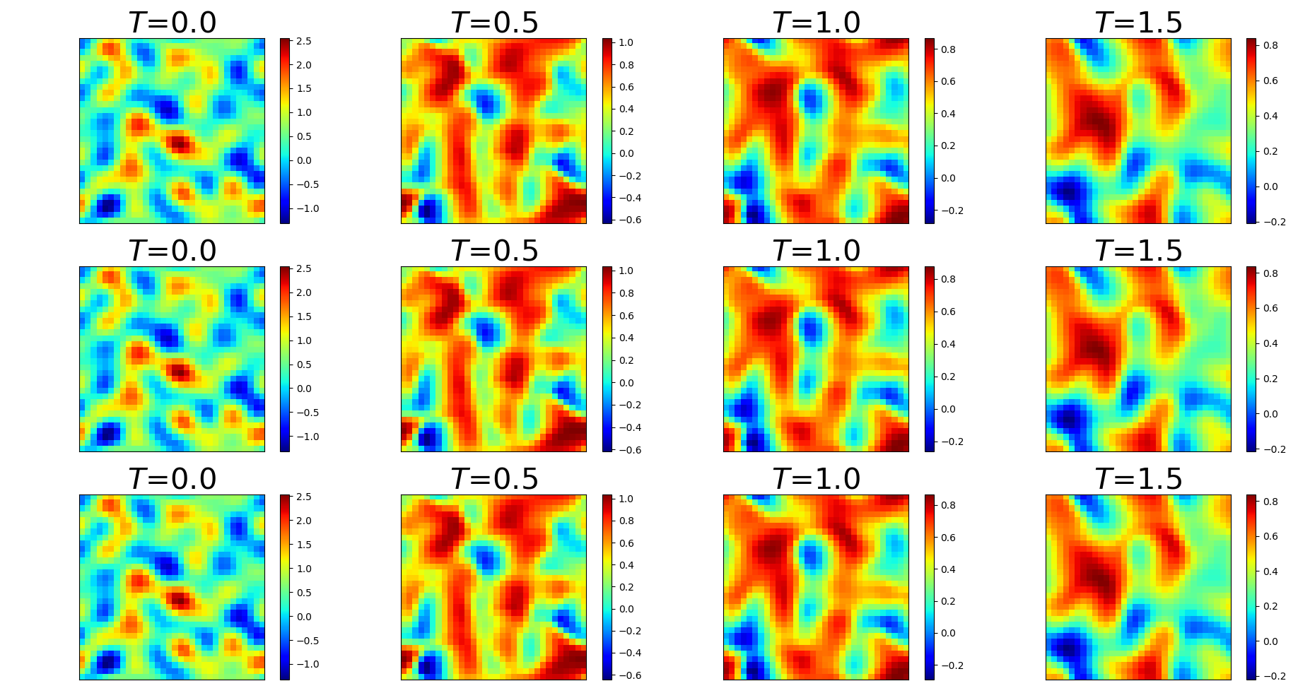
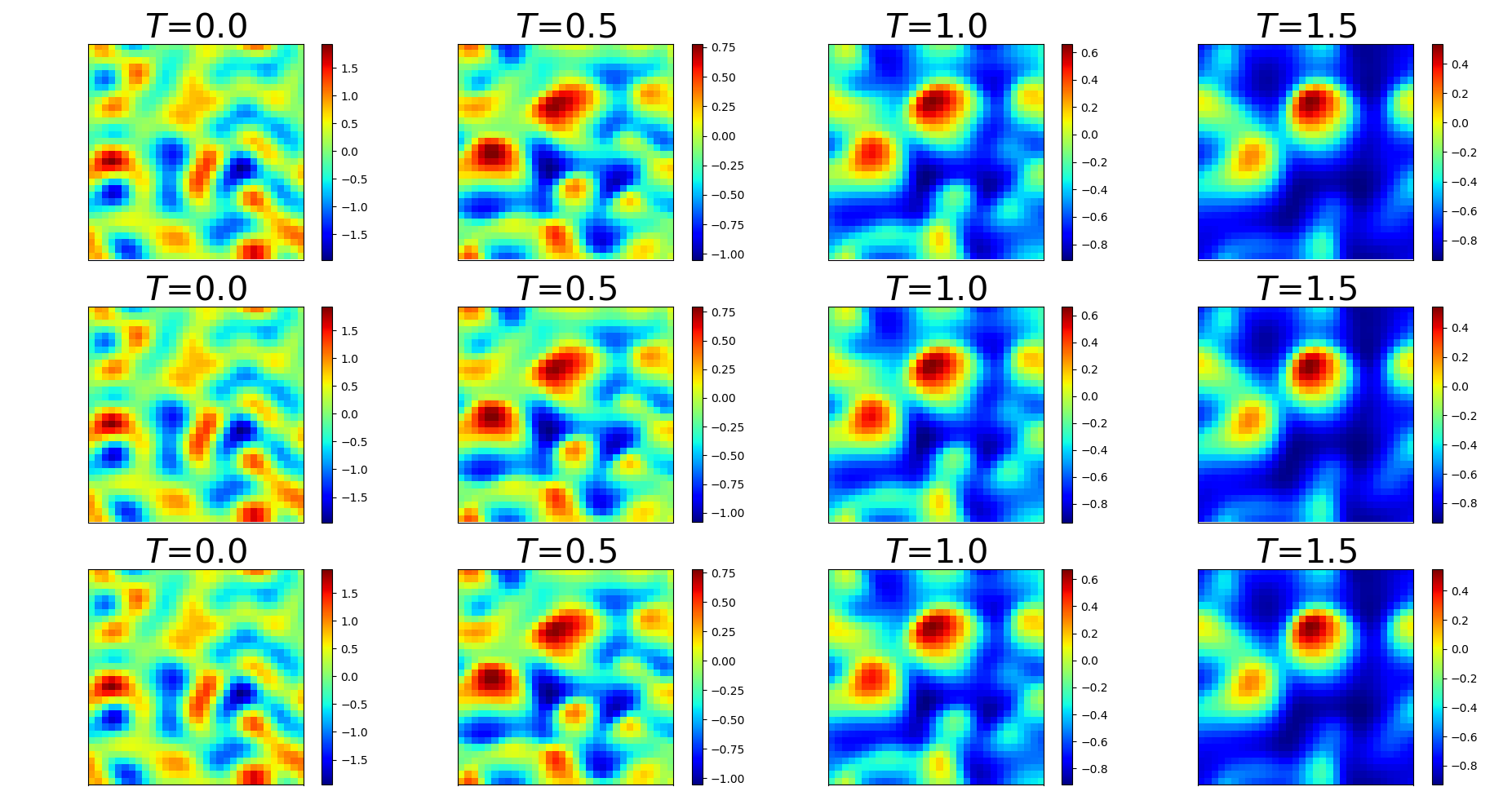
Dynamics of
Dynamics of
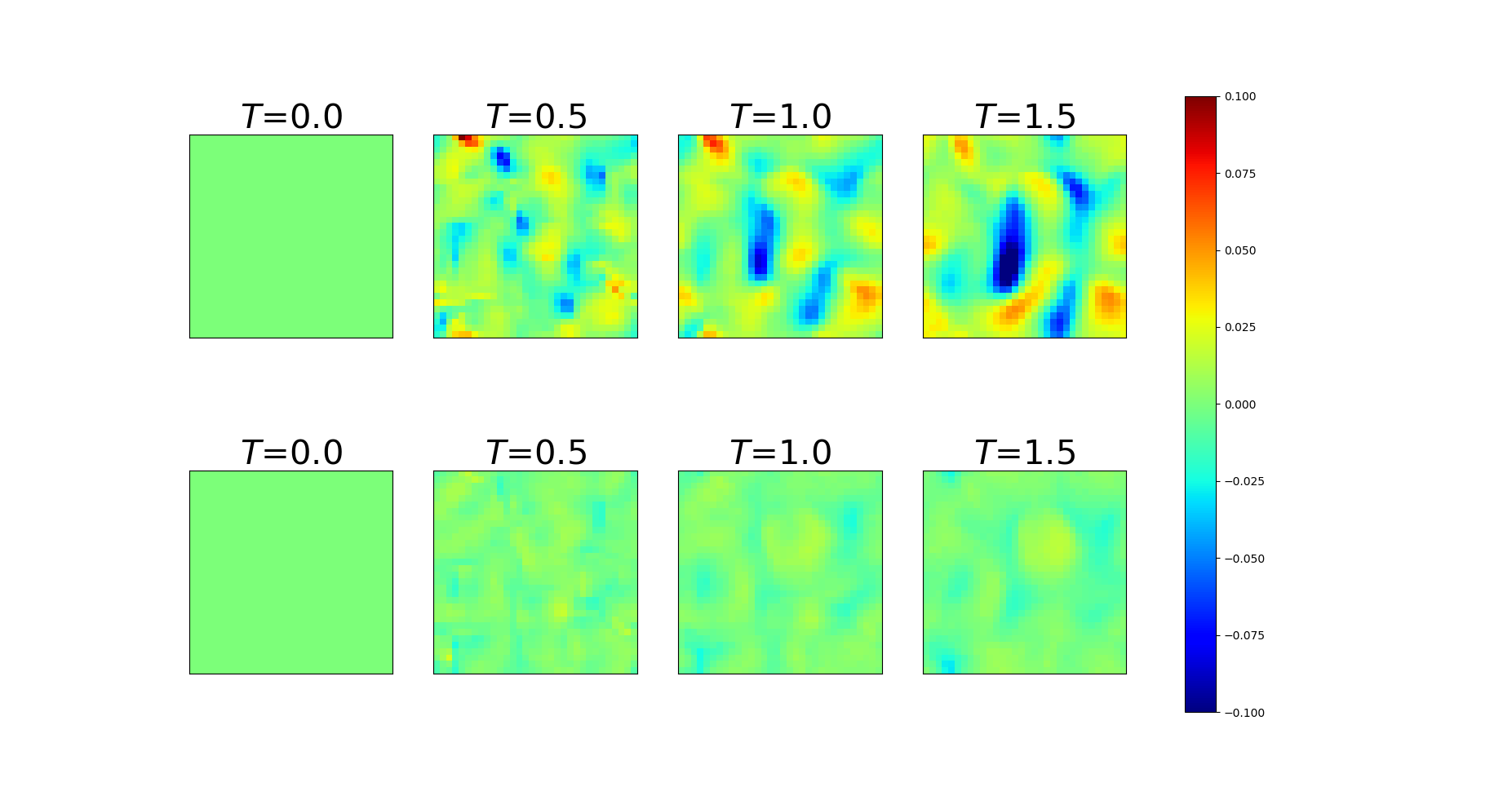
Error maps of
Error maps of
3.3 Importance of and Pseudo-upwind
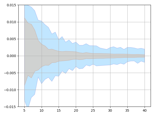
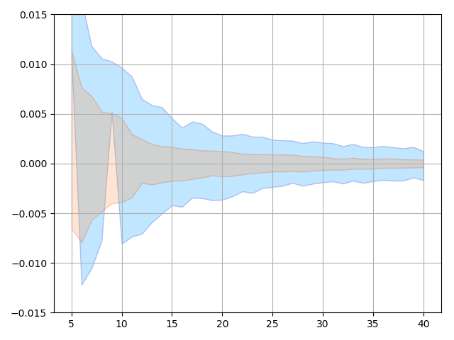
This subsection demonstrates the importance of enforcing sparsity on the and using pseudo-upwind. As we can see from Figure 7 that having sparsity constraints on the helps with suppressing the weights on the terms that do not exist in the Burgers’ equation. Furthermore, Figure 8 and Figure 9 show that having sparsity constraint on the or using pseudo-upwind can significantly reduce prediction errors.


4 Numerical Studies: Diffusion Equation
Diffusion phenomenon has been studied in many applications in physics e.g. the collective motion of micro-particles in materials due to random movement of each particle, or modeling the distribution of temperature in a given region over time.
4.1 Simulated data, training and testing
Consider the 2-dimensional heat equation with periodic boundary condition on
| (13) |
where . The training data of the heat equation is generated by 2nd order Runge-Kutta in time with , and central difference scheme in space on a mesh. We then restrict the data to a mesh. The initial value is also generated from (11).
4.2 Results and discussions
The demonstration on the ability of the trained PDE-Net 2.0 to identify the PDE model is given in Table 2. As one can see from Table 2 that we can recover the terms of the heat equation with good accuracy. Furthermore, all the terms that are not included in the heat equation have much smaller weights in the .
We also demonstrate the ability of the trained PDE-Net 2.0 in prediction. The testing method is exactly the same as the method described in Section 3. Comparisons between PDE-Net 2.0 and Frozen-PDE-Net 2.0 are shown in Figure 10, where we can clearly see the advantage of learning the filters. Visualization of the predicted dynamics is given in Figure 11. All these results show that the learned PDE-Net 2.0 performs well in prediction.
| Correct PDE | |
|---|---|
| Frozen-PDE-Net 2.0 | |
| PDE-Net 2.0 |


5 Numerical Studies: Convection Diffusion Equation with A Reactive Source
Convection diffusion systems are mathematical models which correspond to the transferring of some physical quantities such as energy or materials due to diffusion and convection. Specifically, a convection diffusion system with a reactive source can be used to model a large range of chemical systems in which the transferring of materials competes with productions of materials induced by several chemical reactions.
5.1 Simulated data, training and testing
Consider a 2-dimensional convection diffusion equation with a reactive source and the periodic boundary condition on :
| (14) |
where and . Training data is generated the same way as what we did for Burgers’ equation in Section 3. A 2nd order Runge-Kutta with time step is adopted for temporal discretization. We choose a 2nd order upwind scheme for the convection terms and the central difference scheme for on a mesh. We then restrict the data to a mesh. Noise is added the same way as the Burgers’ equation. The initial values are also generated from (11).
5.2 Results and discussions
The capability of the trained PDE-Net 2.0 to identify the underlying PDE model is demonstrated in Table 3. As one can see that we can recover the terms of the reaction convection diffusion equation with good accuracy. Furthermore, all the terms that are not included in this equation have relatively small weights in the .
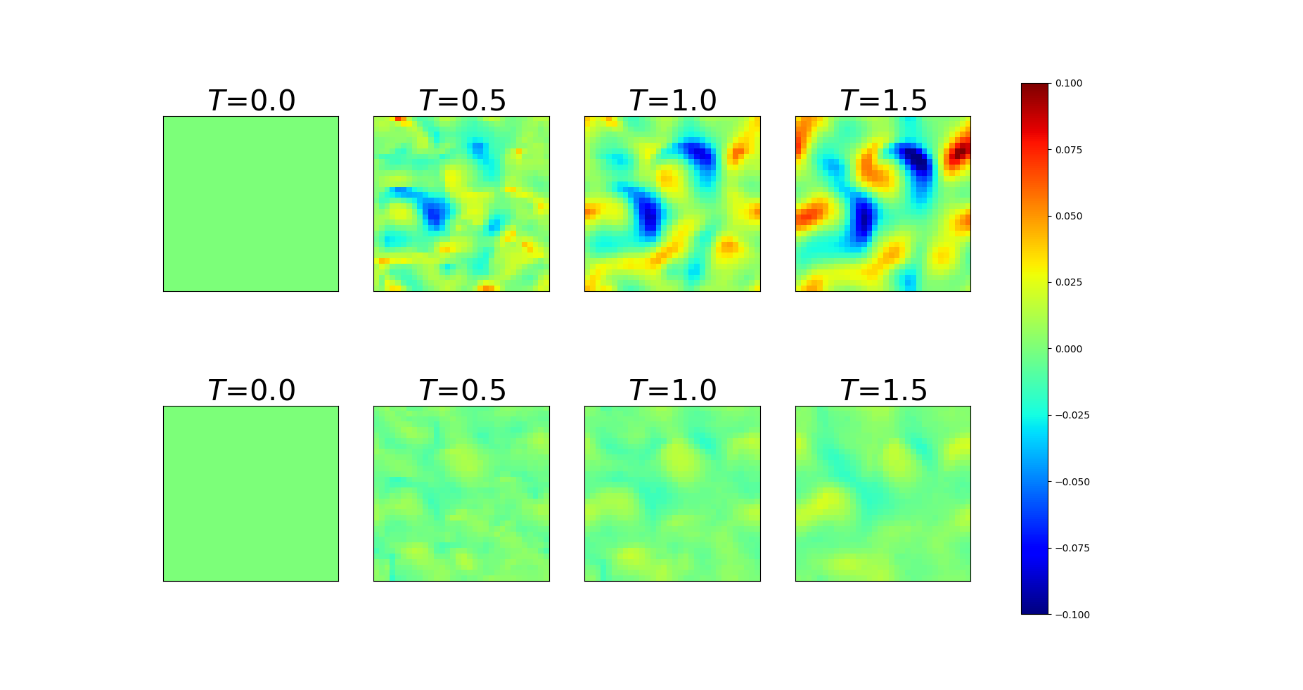
We also demonstrate the ability of the trained PDE-Net 2.0 in prediction. The testing method is exactly the same as the method described in Section 3. Comparisons between PDE-Net 2.0 and Frozen-PDE-Net 2.0 are shown in Figure 12. Visualization of the predicted dynamics and errors maps are given in Figure 13 and Figure 14. Similar to what we observed in Section 3, we can clearly see the benefit from learning discretizations. PDE-Net 2.0 obtains more accurate estimations of the coefficients for the nonlinear convection terms (i.e. the term in Table 3) and makes more accurate predictions (Figure 12) than Frozen-PDE-Net 2.0.
| Correct PDE | |
|---|---|
| Frozen-PDE-Net 2.0 | |
| PDE-Net 2.0 | |


Dynamics of
Dynamics of


Error maps of
Error maps of
6 Conclusions and Future Work
In this paper, we proposed a numeric-symbolic hybrid deep network, called PDE-Net 2.0, for PDE model recovery from observed dynamic data. PDE-Net 2.0 is able to recover the analytic form of the PDE model with minor assumptions on the mechanisms of the observed dynamics. For example, it is able to recover the analytic form of Burgers’ equation with good confidence without any prior knowledge on the type of the equation. Therefore, PDE-Net 2.0 has the potential to uncover potentially new PDEs from observed data. Furthermore, after training, the network can perform accurate long-term prediction without re-training for new initial conditions. The limitations and possible future extensions of the current version of PDE-Net 2.0 is twofold: 1) having only addition and multiplication in the may still be too restrictive, and one may include division as an additional operation in to further improve its expressive power; 2) using forward Euler as temporal discretization is the most straightforward treatment, while a more sophisticated temporal scheme may help with the model recovery and prediction. Both of these worth further exploration. Furthermore, we would like to apply the network to real biological dynamic data. We will further investigate the reliability of the network and explore the possibility to uncover new dynamical principles that have meaningful scientific explanations.
Acknowledgments
Zichao Long is supported by The Elite Program of Computational and Applied Mathematics for PhD Candidates of Peking University. Yiping Lu is supported by the Elite Undergraduate Training Program of the School of Mathematical Sciences at Peking University. Bin Dong is supported in part by Beijing Natural Science Foundation (No. 180001) and Beijing Academy of Artificial Intelligence (BAAI).
References
- [1] Zichao Long, Yiping Lu, Xianzhong Ma, and Bin Dong. Pde-net: Learning pdes from data. In International Conference on Machine Learning, pages 3214–3222, 2018.
- [2] Christopher Earls Brennen and Christopher E Brennen. Fundamentals of multiphase flow. Cambridge university press, 2005.
- [3] Messoud Efendiev. Mathematical modeling of mitochondrial swelling.
- [4] Josh Bongard and Hod Lipson. Automated reverse engineering of nonlinear dynamical systems. Proceedings of the National Academy of Sciences, 104(24):9943–9948, 2007.
- [5] Michael Schmidt and Hod Lipson. Distilling free-form natural laws from experimental data. science, 324(5923):81–85, 2009.
- [6] Maziar Raissi and George Em Karniadakis. Hidden physics models: Machine learning of nonlinear partial differential equations. Journal of Computational Physics, 357:125–141, 2018.
- [7] Maziar Raissi, Paris Perdikaris, and George Em Karniadakis. Physics informed deep learning (part ii): data-driven discovery of nonlinear partial differential equations. arXiv preprint arXiv:1711.10566, 2017.
- [8] Steven L Brunton, Joshua L Proctor, and J Nathan Kutz. Discovering governing equations from data by sparse identification of nonlinear dynamical systems. Proceedings of the National Academy of Sciences, page 201517384, 2016.
- [9] Hayden Schaeffer. Learning partial differential equations via data discovery and sparse optimization. Proc. R. Soc. A, 473(2197):20160446, 2017.
- [10] Samuel H Rudy, Steven L Brunton, Joshua L Proctor, and J Nathan Kutz. Data-driven discovery of partial differential equations. Science Advances, 3(4):e1602614, 2017.
- [11] Haibin Chang and Dongxiao Zhang. Identification of physical processes via combined data-driven and data-assimilation methods. arXiv preprint arXiv:1810.11977, 2018.
- [12] Hayden Schaeffer, Giang Tran, Rachel Ward, and Linan Zhang. Extracting structured dynamical systems using sparse optimization with very few samples. arXiv preprint arXiv:1805.04158, 2018.
- [13] Zongmin Wu and Ran Zhang. Learning physics by data for the motion of a sphere falling in a non-newtonian fluid. Communications in Nonlinear Science and Numerical Simulation, 67:577–593, 2019.
- [14] Emmanuel de Bezenac, Arthur Pajot, and Patrick Gallinari. Deep learning for physical processes: Incorporating prior scientific knowledge. arXiv preprint arXiv:1711.07970, 2017.
- [15] Kaiming He, Xiangyu Zhang, Shaoqing Ren, and Jian Sun. Deep residual learning for image recognition. In Proceedings of the IEEE conference on computer vision and pattern recognition, pages 770–778, 2016.
- [16] Kaiming He, Xiangyu Zhang, Shaoqing Ren, and Jian Sun. Identity mappings in deep residual networks. In European conference on computer vision, pages 630–645. Springer, 2016.
- [17] Yunjin Chen, Wei Yu, and Thomas Pock. On learning optimized reaction diffusion processes for effective image restoration. In Proceedings of the IEEE conference on computer vision and pattern recognition, pages 5261–5269, 2015.
- [18] E Weinan. A proposal on machine learning via dynamical systems. Communications in Mathematics and Statistics, 5(1):1–11, 2017.
- [19] Eldad Haber and Lars Ruthotto. Stable architectures for deep neural networks. Inverse Problems, 34(1):014004, 2017.
- [20] Sho Sonoda and Noboru Murata. Double continuum limit of deep neural networks. In ICML Workshop Principled Approaches to Deep Learning, 2017.
- [21] Yiping Lu, Aoxiao Zhong, Quanzheng Li, and Bin Dong. Beyond finite layer neural networks: Bridging deep architectures and numerical differential equations. In International Conference on Machine Learning, pages 3282–3291, 2018.
- [22] Bo Chang, Lili Meng, Eldad Haber, Frederick Tung, and David Begert. Multi-level residual networks from dynamical systems view. In ICLR, 2018.
- [23] Tian Qi Chen, Yulia Rubanova, Jesse Bettencourt, and David Duvenaud. Neural ordinary differential equations. arXiv preprint arXiv:1806.07366, 2018.
- [24] Tong Qin, Kailiang Wu, and Dongbin Xiu. Data driven governing equations approximation using deep neural networks. arXiv preprint arXiv:1811.05537, 2018.
- [25] Steffen Wiewel, Moritz Becher, and Nils Thuerey. Latent-space physics: Towards learning the temporal evolution of fluid flow. arXiv preprint arXiv:1802.10123, 2018.
- [26] Byungsoo Kim, Vinicius C Azevedo, Nils Thuerey, Theodore Kim, Markus Gross, and Barbara Solenthaler. Deep fluids: A generative network for parameterized fluid simulations. arXiv preprint arXiv:1806.02071, 2018.
- [27] Karthikeyan Duraisamy, Ze J Zhang, and Anand Pratap Singh. New approaches in turbulence and transition modeling using data-driven techniques. In 53rd AIAA Aerospace Sciences Meeting, page 1284, 2015.
- [28] Karthik Duraisamy, Gianluca Iaccarino, and Heng Xiao. Turbulence modeling in the age of data. Annual Review of Fluid Mechanics, 51:357–377, 2019.
- [29] Chao Ma, Jianchun Wang, et al. Model reduction with memory and the machine learning of dynamical systems. arXiv preprint arXiv:1808.04258, 2018.
- [30] WG Noid, Jhih-Wei Chu, Gary S Ayton, Vinod Krishna, Sergei Izvekov, Gregory A Voth, Avisek Das, and Hans C Andersen. The multiscale coarse-graining method. i. a rigorous bridge between atomistic and coarse-grained models. The Journal of chemical physics, 128(24):244114, 2008.
- [31] Linfeng Zhang, Jiequn Han, Han Wang, Roberto Car, and E Weinan. Deep potential molecular dynamics: a scalable model with the accuracy of quantum mechanics. Physical review letters, 120(14):143001, 2018.
- [32] Jian-Feng Cai, Bin Dong, Stanley Osher, and Zuowei Shen. Image restoration: total variation, wavelet frames, and beyond. Journal of the American Mathematical Society, 25(4):1033–1089, 2012.
- [33] Bin Dong, Qingtang Jiang, and Zuowei Shen. Image restoration: Wavelet frame shrinkage, nonlinear evolution pdes, and beyond. Multiscale Modeling & Simulation, 15(1):606–660, 2017.
- [34] Ingrid Daubechies. Ten lectures on wavelets, volume 61. Siam, 1992.
- [35] Stéphane Mallat. A wavelet tour of signal processing. Elsevier, 1999.
- [36] Tomaso Poggio, Hrushikesh Mhaskar, Lorenzo Rosasco, Brando Miranda, and Qianli Liao. Why and when can deep-but not shallow-networks avoid the curse of dimensionality: a review. International Journal of Automation and Computing, 14(5):503–519, 2017.
- [37] Uri Shaham, Alexander Cloninger, and Ronald R Coifman. Provable approximation properties for deep neural networks. Applied and Computational Harmonic Analysis, 2016.
- [38] Hadrien Montanelli and Qiang Du. Deep relu networks lessen the curse of dimensionality. arXiv preprint arXiv:1712.08688, 2017.
- [39] Qingcan Wang et al. Exponential convergence of the deep neural network approximation for analytic functions. arXiv preprint arXiv:1807.00297, 2018.
- [40] Juncai He, Lin Li, Jinchao Xu, and Chunyue Zheng. Relu deep neural networks and linear finite elements. arXiv preprint arXiv:1807.03973, 2018.
- [41] Georg Martius and Christoph H Lampert. Extrapolation and learning equations. arXiv preprint arXiv:1610.02995, 2016.
- [42] Subham Sahoo, Christoph Lampert, and Georg Martius. Learning equations for extrapolation and control. In International Conference on Machine Learning, pages 4439–4447, 2018.
- [43] Xu-Dong Liu, Stanley Osher, and Tony Chan. Weighted essentially non-oscillatory schemes. Journal of computational physics, 115(1):200–212, 1994.
- [44] Chi-Wang Shu. Essentially non-oscillatory and weighted essentially non-oscillatory schemes for hyperbolic conservation laws. In Advanced numerical approximation of nonlinear hyperbolic equations, pages 325–432. Springer, 1998.
- [45] Randall J LeVeque. Finite volume methods for hyperbolic problems, volume 31. Cambridge university press, 2002.