PEAR: Primitive enabled Adaptive
Relabeling for boosting Hierarchical
Reinforcement Learning
Abstract
Hierarchical reinforcement learning (HRL) has the potential to solve complex long horizon tasks using temporal abstraction and increased exploration. However, hierarchical agents are difficult to train due to inherent non-stationarity. We present primitive enabled adaptive relabeling (PEAR), a two-phase approach where we first perform adaptive relabeling on a few expert demonstrations to generate efficient subgoal supervision, and then jointly optimize HRL agents by employing reinforcement learning (RL) and imitation learning (IL). We perform theoretical analysis to bound the sub-optimality of our approach and derive a joint optimization framework using RL and IL. Since PEAR utilizes only a few expert demonstrations and considers minimal limiting assumptions on the task structure, it can be easily integrated with typical off-policy RL algorithms to produce a practical HRL approach. We perform extensive experiments on challenging environments and show that PEAR is able to outperform various hierarchical and non-hierarchical baselines and achieve upto success rates in complex sparse robotic control tasks where other baselines typically fail to show significant progress. We also perform ablations to thoroughly analyse the importance of our various design choices. Finally, we perform real world robotic experiments on complex tasks and demonstrate that PEAR consistently outperforms the baselines.
1 Introduction
Reinforcement learning has been successfully applied to a number of short-horizon robotic manipulation tasks (Rajeswaran et al., 2018; Kalashnikov et al., 2018; Gu et al., 2017; Levine et al., 2016). However, solving long horizon tasks requires long-term planning and is hard (Gupta et al., 2019) due to inherent issues like credit assignment and ineffective exploration. Consequently, such tasks require a large number of environment interactions for learning, especially in sparse reward scenarios (Andrychowicz et al., 2017). Hierarchical reinforcement learning (HRL) (Sutton et al., 1999; Dayan and Hinton, 1993; Vezhnevets et al., 2017; Klissarov et al., 2017; Bacon et al., 2017) is an elegant framework that employs temporal abstraction and promises improved exploration (Nachum et al., 2019). In goal-conditioned feudal architecture (Dayan and Hinton, 1993; Vezhnevets et al., 2017), the higher policy predicts subgoals for the lower primitive, which in turn tries to achieve these subgoals by executing primitive actions directly on the environment. Unfortunately, HRL suffers from non-stationarity (Nachum et al., 2018; Levy et al., 2018) in off-policy HRL. Due to continuously changing policies, previously collected off-policy experience is rendered obsolete, leading to unstable higher level state transition and reward functions.
Some hierarchical approaches (Gupta et al., 2019; Fox et al., 2017; Krishnan et al., 2019) segment the expert demonstrations into subgoal transition dataset, and consequently leverage the subgoal dataset to bootstrap learning. Ideally, the segmentation process should produce subgoals that properly balance the task split between hierarchical levels. One possible approach of task segmentation is to perform fixed window based relabeling (Gupta et al., 2019) on expert demonstrations. Despite being simple, this is effectively a brute force segmentation approach which may generate subgoals that are either too easy or too hard according to the current goal achieving ability of the lower primitive, thus leading to degenerate solutions.
The main motivation of this work is to produce a curriculum of feasible subgoals according to the current goal achieving capability of the lower primitive. Concretely, the value function of the lower primitive is used to perform adaptive relabeling on expert demonstrations to dynamically generate a curriculum of achievable subgoals for the lower primitive. This subgoal dataset is then used to train an imitation learning based regularizer, which is used to jointly optimize off-policy RL objective with IL regularization. Hence, our approach ameliorates non-stationarity in HRL by using primitive enabled IL regularization, while enabling efficient exploration using RL. We call our approach: primitive enabled adaptive relabeling (PEAR) for boosting HRL.
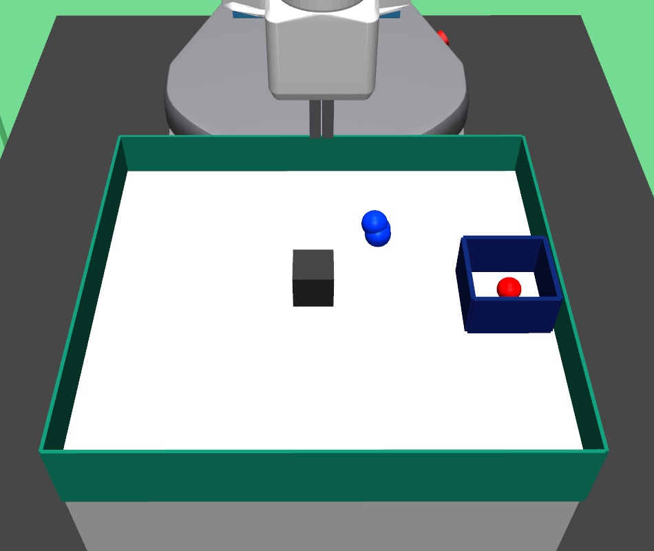
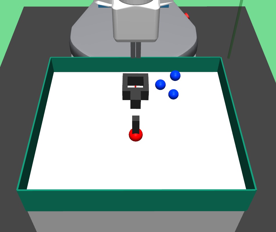
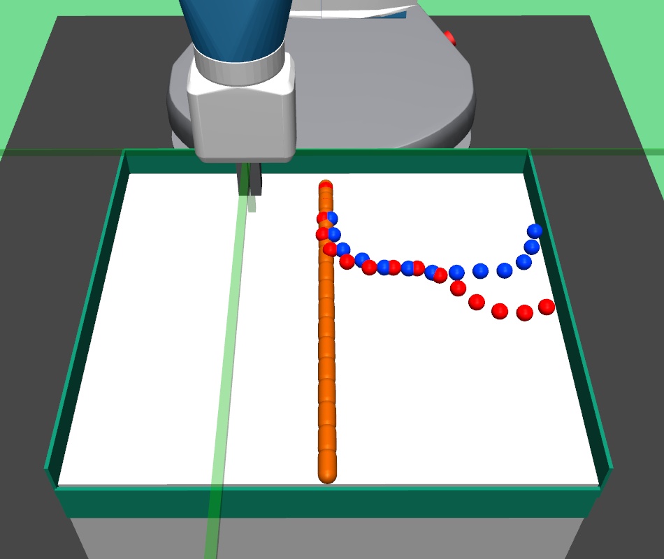
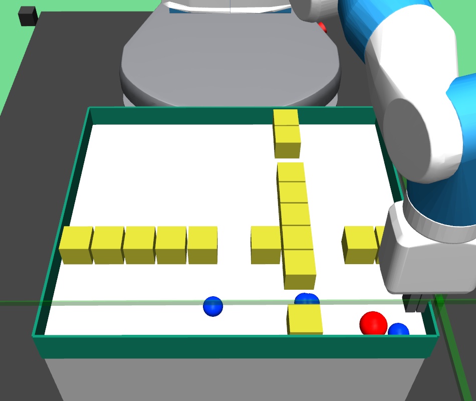
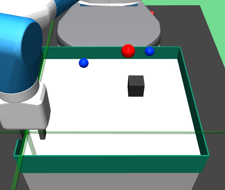
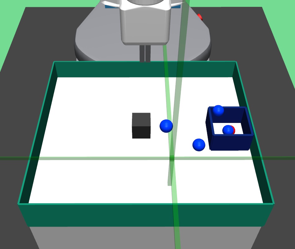
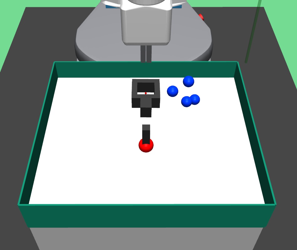
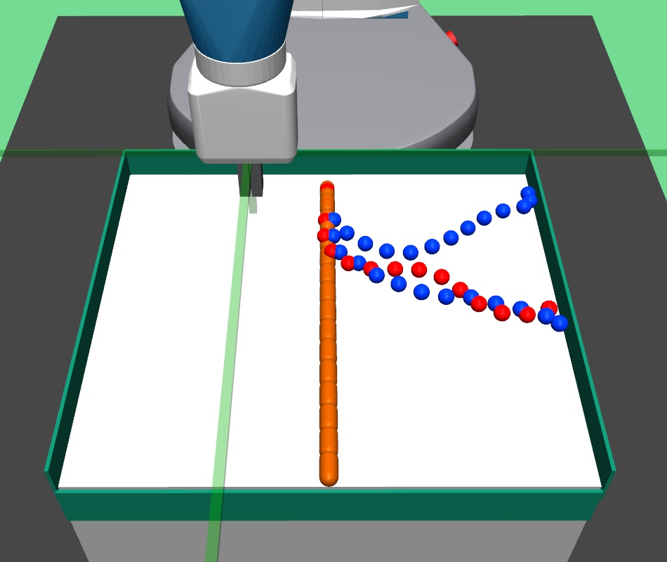
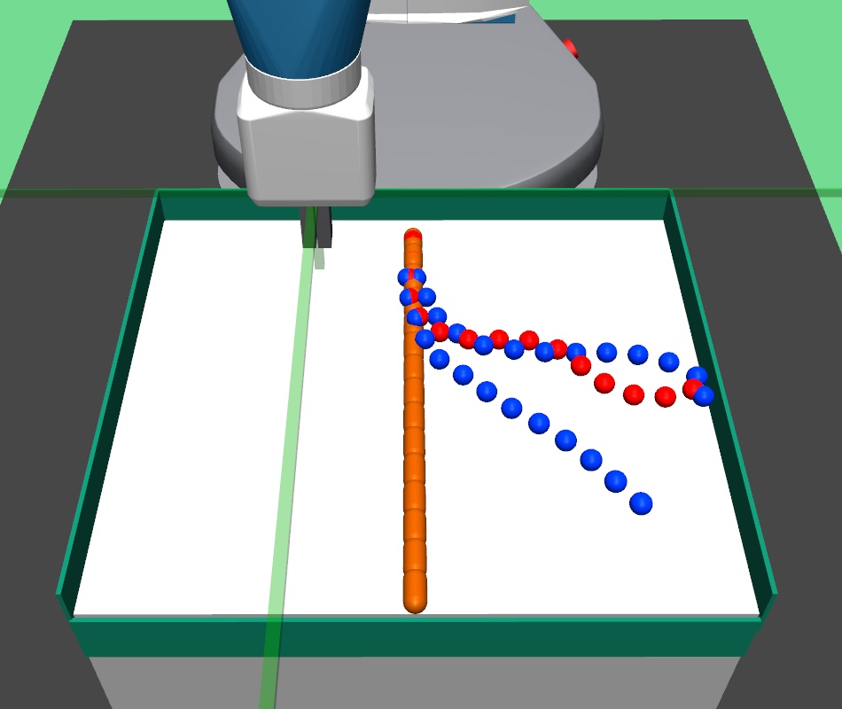
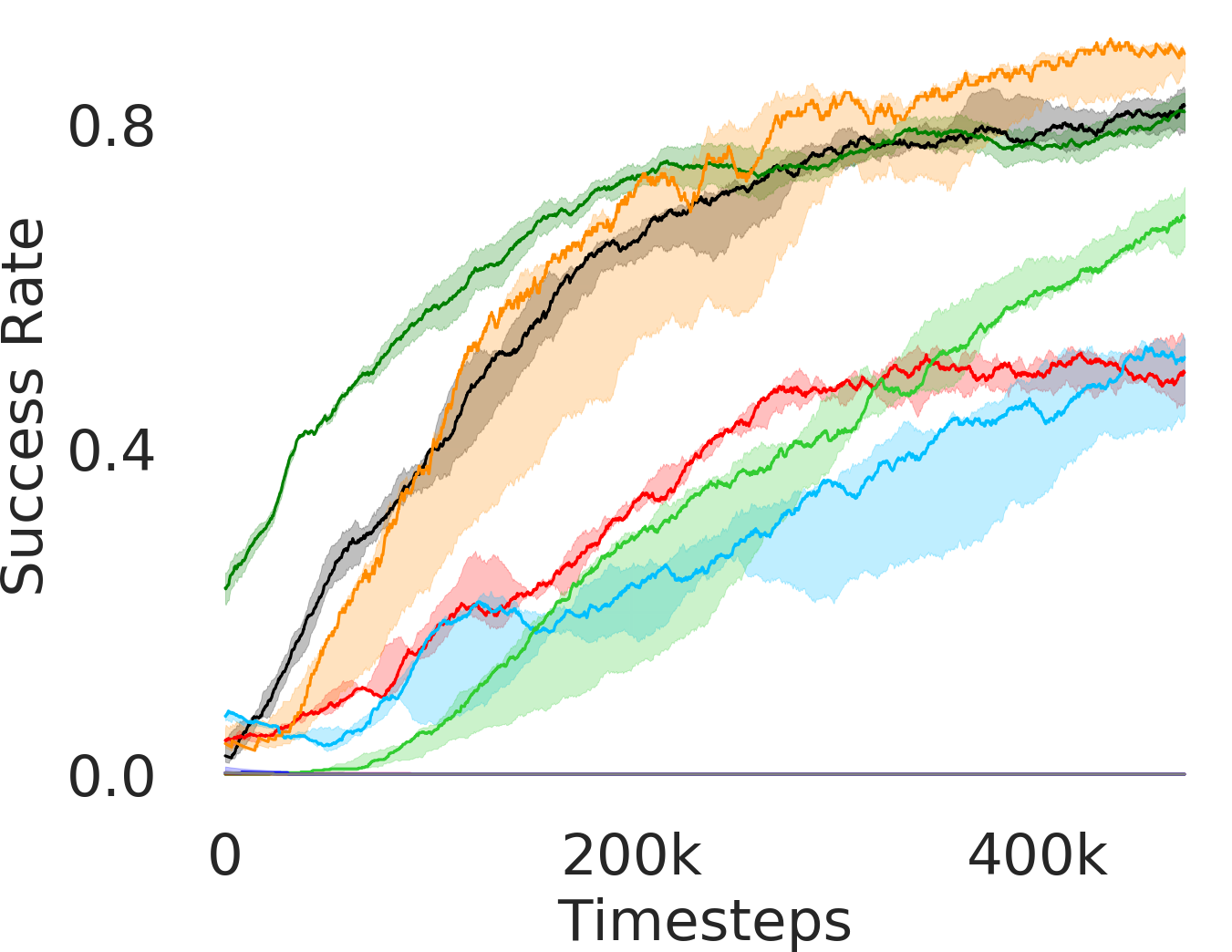
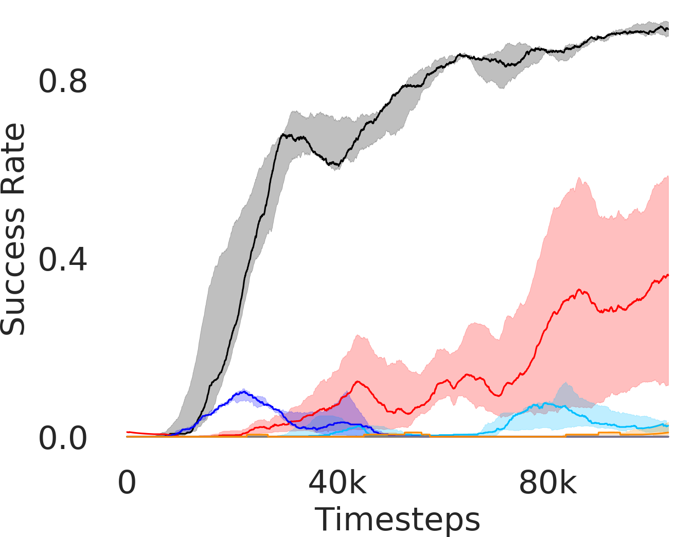
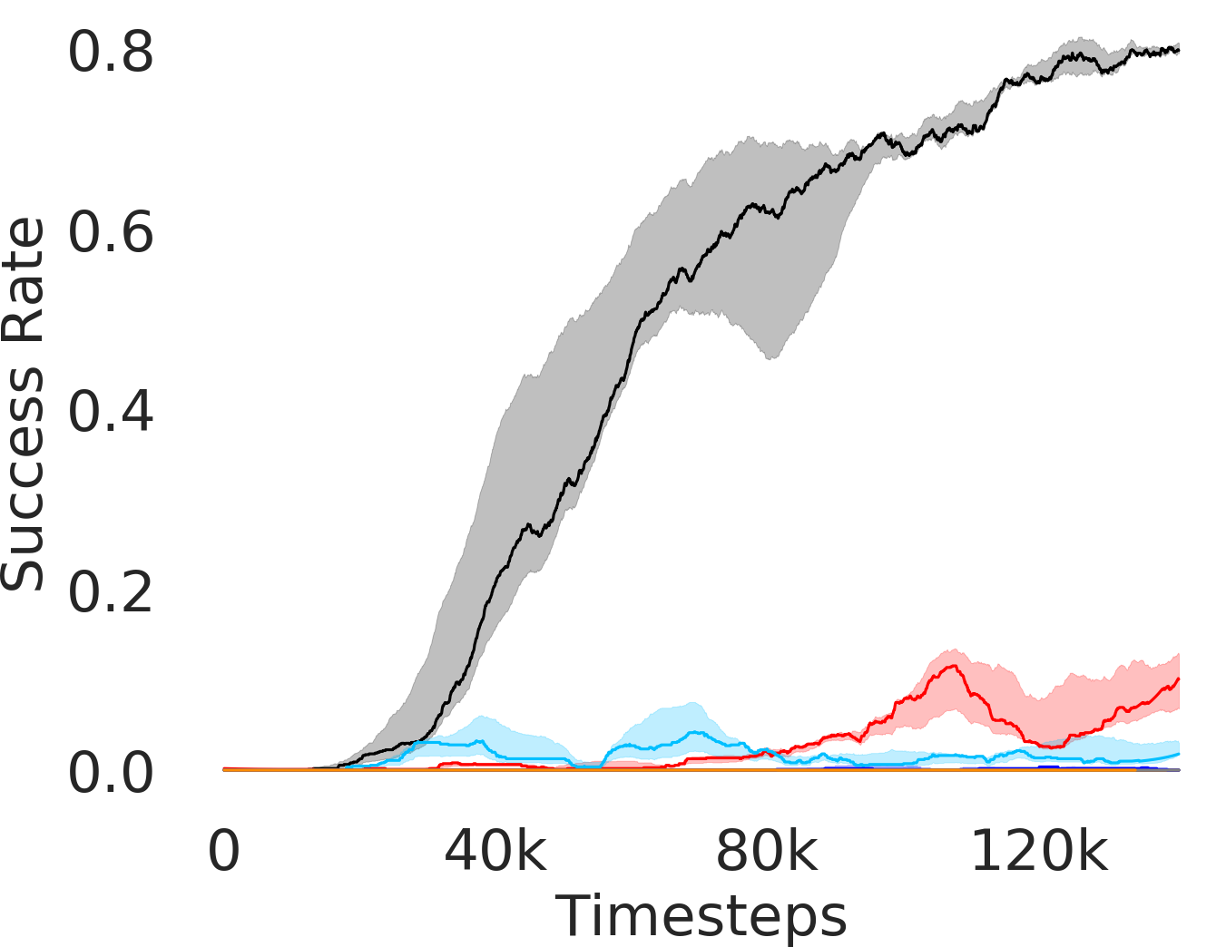
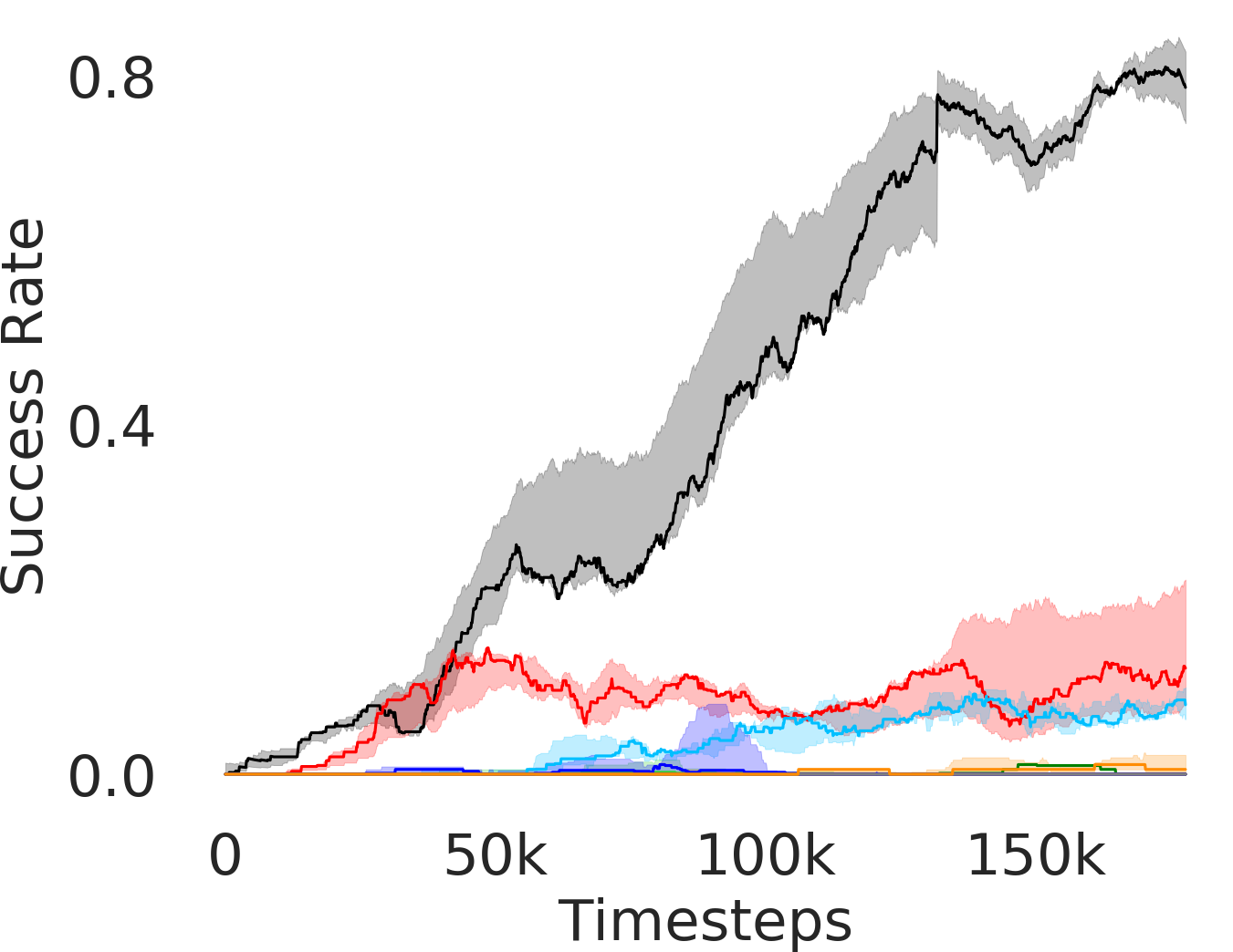
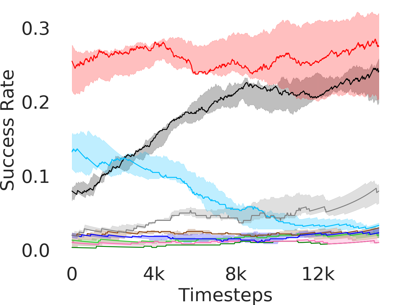
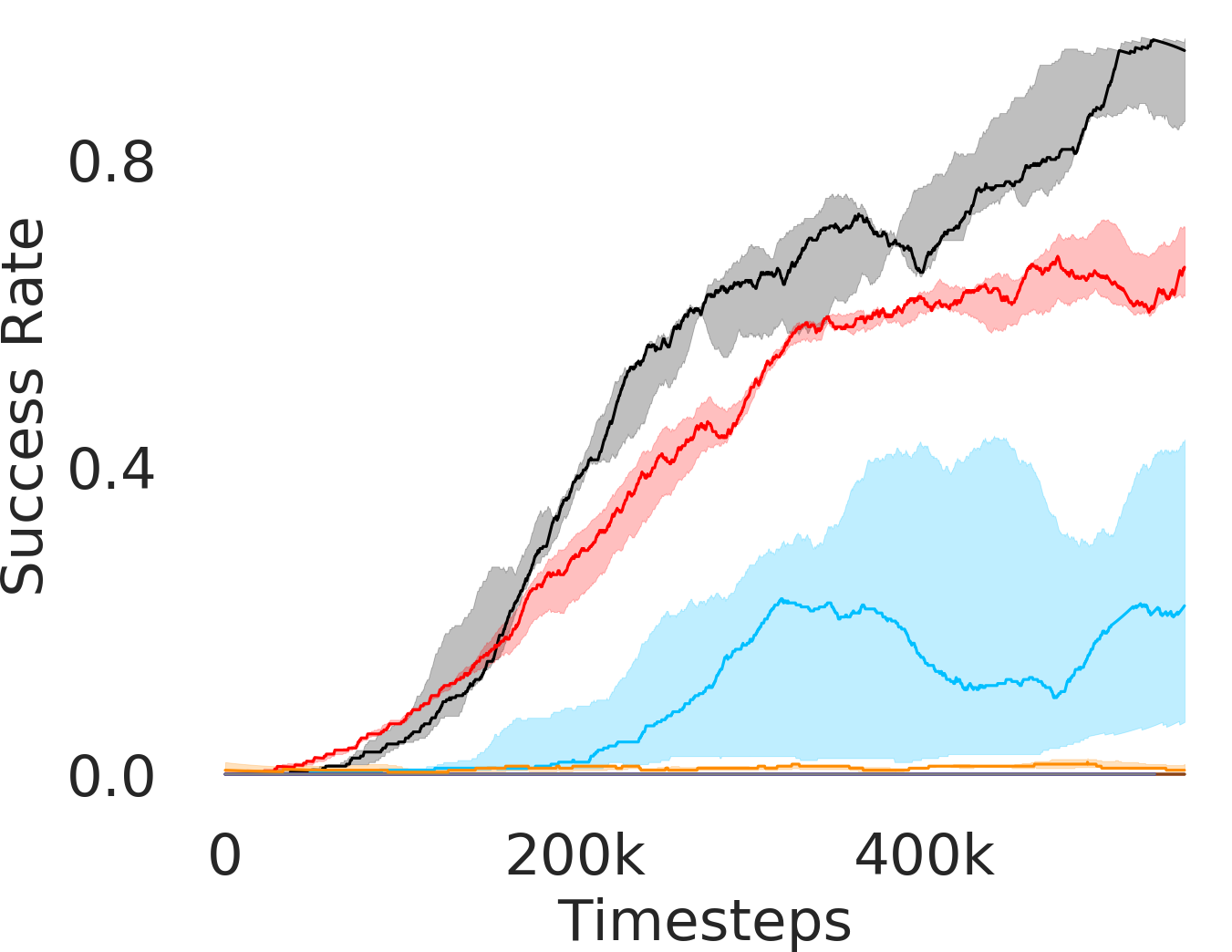
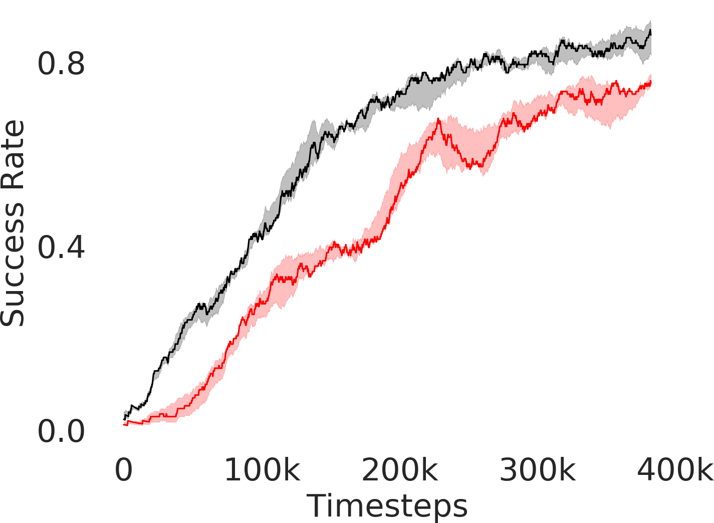
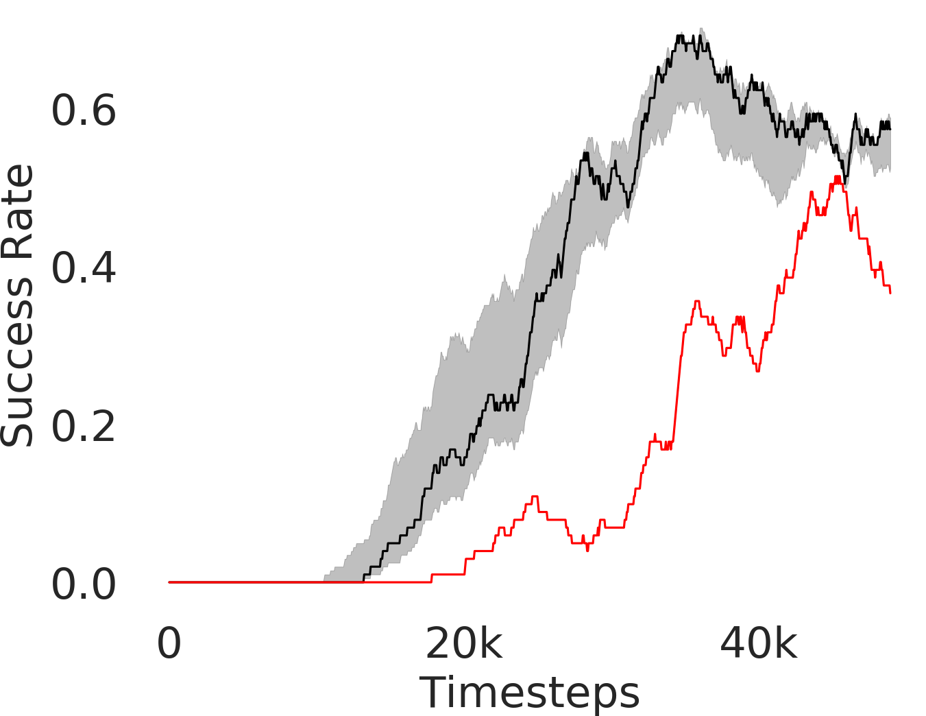
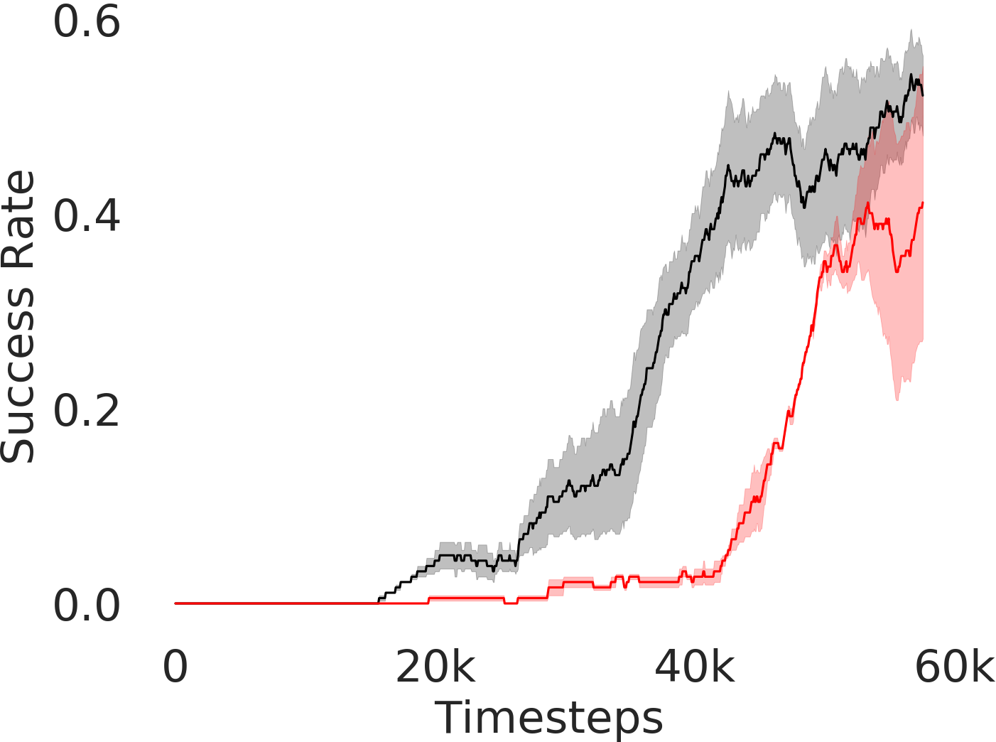
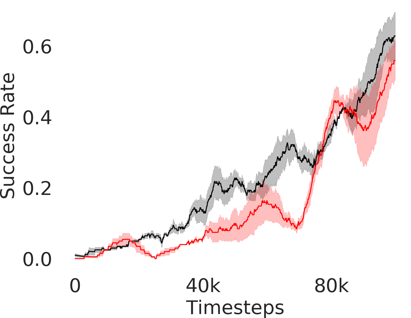
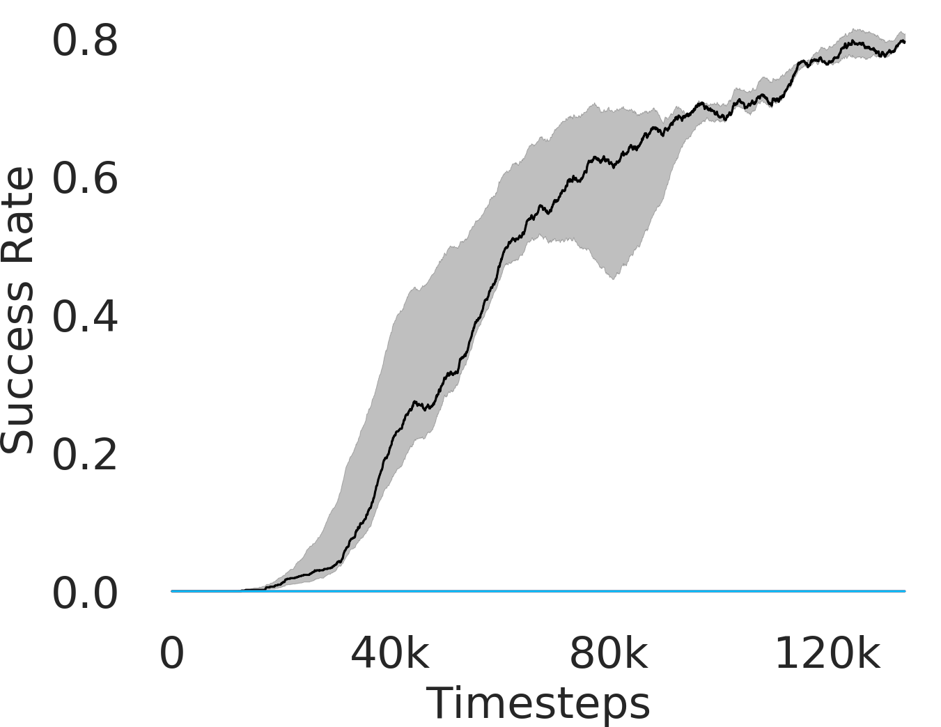
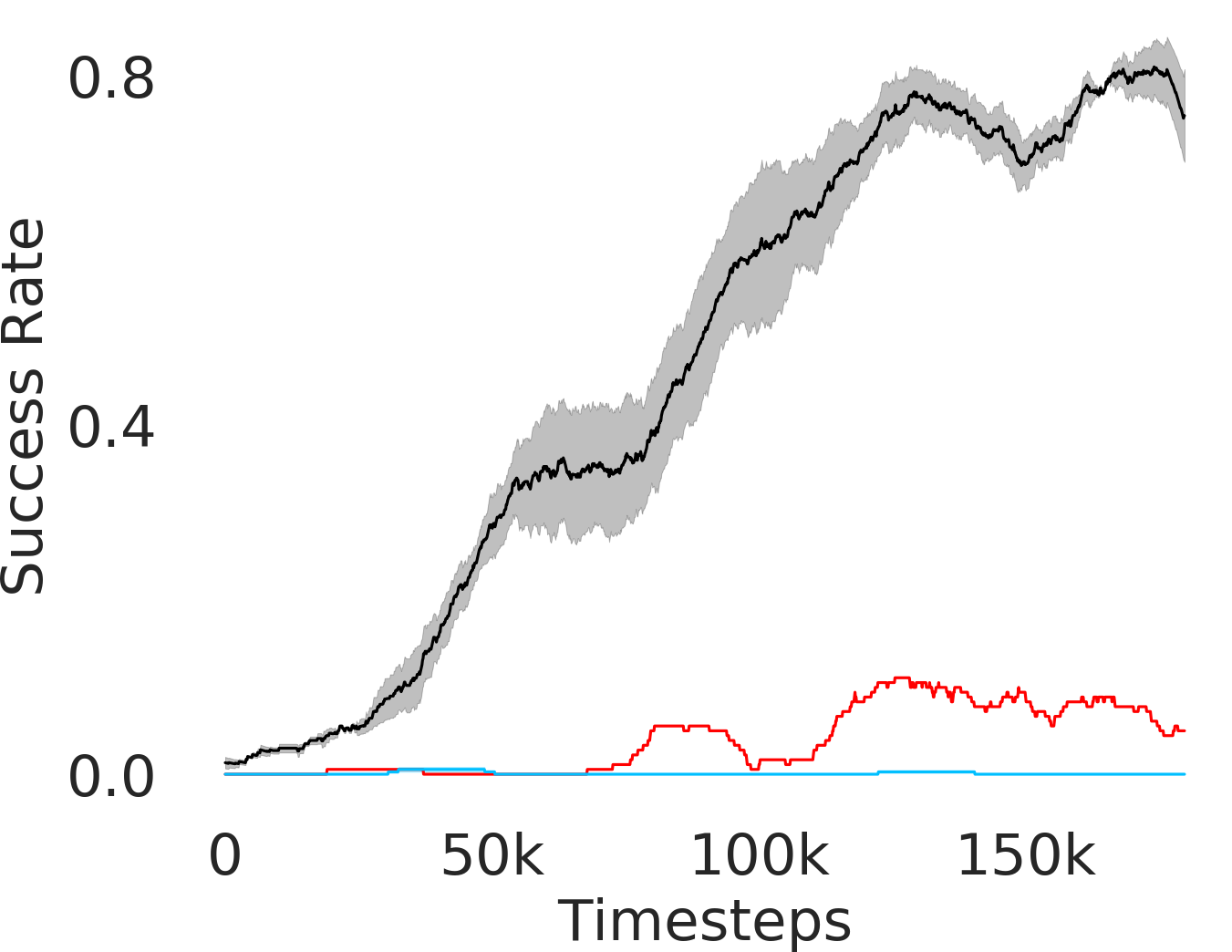
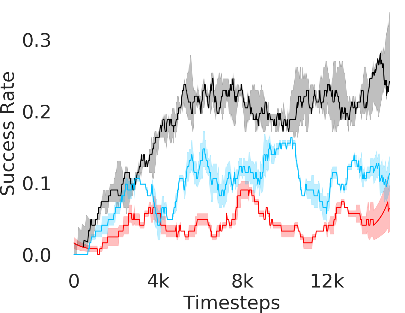
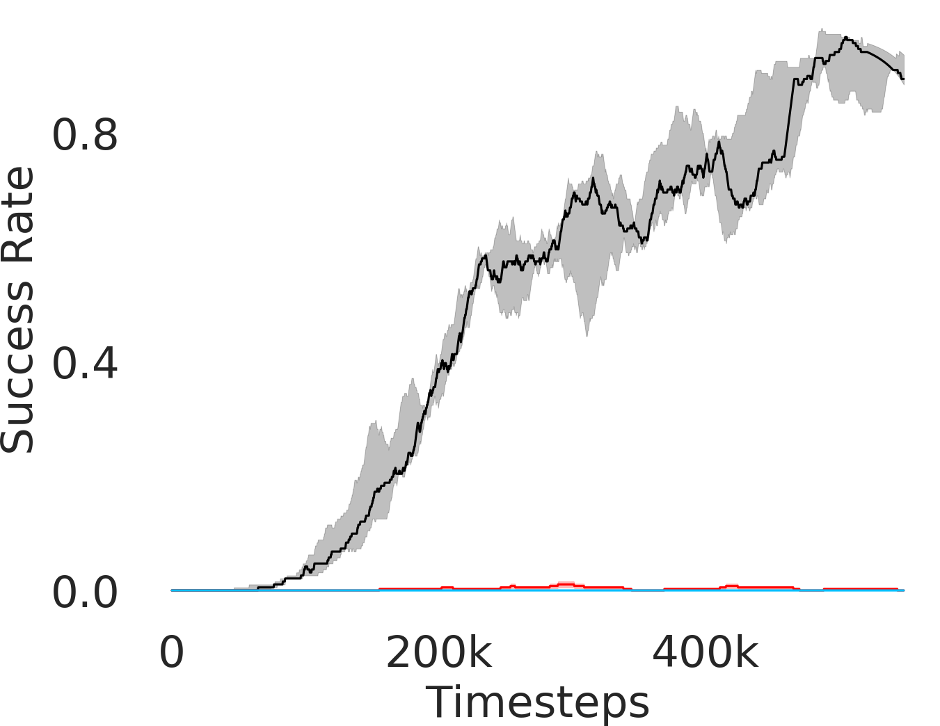
The major contributions of this work are: our adaptive relabeling based approach generates efficient higher level subgoal supervision according to the current goal achieving capability of the lower primitive (Figure 2), we derive sub-optimality bounds to theoretically justify the benefits of periodic re-population using adaptive relabeling (Section 4.3), we perform extensive experimentation on sparse robotic tasks: maze navigation, pick and place, bin, hollow, rope manipulation and franka kitchen to empirically demonstrate superior performance and sample efficiency of PEAR over prior baselines (Section 5 Figure 3), and finally, we show that PEAR demonstrates impressive performance in real world tasks: pick and place, bin and rope manipulation (Figure 6).
2 Related Work
Hierarchical reinforcement learning (HRL) (Barto and Mahadevan, 2003; Sutton et al., 1999; Parr and Russell, 1998; Dietterich, 2000) promises the advantages of temporal abstraction and increased exploration (Nachum et al., 2019). The options architecture (Sutton et al., 1999; Bacon et al., 2017; Harutyunyan et al., 2018; Harb et al., 2018; Harutyunyan et al., 2019; Klissarov et al., 2017) learns temporally extended macro actions and a termination function to propose an elegant hierarchical framework. However, such approaches may produce degenerate solutions in the absence of proper regularization. Some approaches restrict the problem search space by greedily solving for specific goals (Kaelbling, 1993; Foster and Dayan, 2002), which has also been extended to hierarchical RL (Wulfmeier et al., 2019; 2021; Ding et al., 2019). In goal-conditioned feudal learning (Dayan and Hinton, 1993; Vezhnevets et al., 2017), the higher level agent produces subgoals for the lower primitive, which in turn executes atomic actions on the environment. Unfortunately, off-policy HRL approaches are cursed by non-stationarity issue. Prior works (Nachum et al., 2018; Levy et al., 2018) deal with the non-stationarity by relabeling previously collected transitions for training goal-conditioned policies. In contrast, our proposed approach deals with non-stationarity by leveraging adaptive relabeling for periodically producing achievable subgoals, and subsequently using an imitation learning based regularizer. We empirically show in Section 5 that our regularization based approach outperforms relabeling based hierarchical approaches on various long horizon tasks.
Prior methods (Rajeswaran et al., 2018; Nair et al., 2018; Hester et al., 2018) leverage expert demonstrations to improve sample efficiency and accelerate learning, where some methods use imitation learning to bootstrap learning (Shiarlis et al., 2018; Krishnan et al., 2017; 2019; Kipf et al., 2019). Some approaches use fixed relabeling (Gupta et al., 2019) for performing task segmentation. However, such approaches may cause unbalanced task split between hierarchical levels. In contrast, our approach sidesteps this limitation by properly balancing hierarchical levels using adaptive relabeling. Intuitively, we enable balanced task split, thereby avoiding degenerate solutions. Recent approaches restrict subgoal space using adjacency constraints (Zhang et al., 2020), employ graph based approaches for decoupling task horizon (Lee et al., 2023), or incorporate imagined subgoals combined with KL-constrained policy iteration scheme (Chane-Sane et al., 2021). However, such approaches assume additional environment constraints and only work on relatively shorter horizon tasks with limited complexity. (Kreidieh et al., 2020) is an inter-level cooperation based approach for generating achievable subgoals, However, the approach requires extensive exploration for selecting good subgoals, whereas our approach rapidly enables effective subgoal generation using primitive enabled adaptive relabeling. In order to accelerate RL, recent works firstly learn behavior skill priors (Pertsch et al., 2020; Singh et al., 2021) from expert data or pre-train policies over a related task, and then fine-tune using RL. Such approaches largely depend on policies learnt during pre-training, and are hard to train when the source and target task distributions are dissimilar. Other approaches either use bottleneck option discovery (Salter et al., 2022b) or behavior priors (Salter et al., 2022a; Tirumala et al., 2022) to discover and embed behaviors from past experience, or directly hand-design action primitives (Dalal et al., 2021; Nasiriany et al., 2022). While this simplifies the higher level task, explicitly designing action primitives is tedious for hard tasks, and may lead to sub-optimal predictions. Since PEAR learns multi-level policies in parallel, the lower level policies can learn required optimal behavior, thus avoiding the issues with prior approaches.
3 Background
Off-policy Reinforcement Learning We define our goal-conditioned off-policy RL setup as follows: Universal Markov Decision Process (UMDP) (Schaul et al., 2015) is a Markov decision process augmented with the goal space , where . Here, is state space, is action space, is the state transition probability function, is reward function, and is discount factor. represents the goal-conditioned policy which predicts the probability of taking action when the state is and goal is . The overall objective is to maximize expected future discounted reward distribution: .
Hierarchical Reinforcement Learning In our goal-conditioned HRL setup, the overall policy is divided into multi-level policies. We consider bi-level scheme, where the higher level policy predicts subgoals for the lower primitive . generates subgoals after every timesteps and tries to achieve within timesteps. gets sparse extrinsic reward from the environment, whereas gets sparse intrinsic reward from . gets rewarded with reward if the agent reaches within distance of the predicted subgoal , and otherwise: . Similarly, gets extrinsic reward if the achieved goal is within distance of the final goal , and otherwise: . We assume access to a small number of directed expert demonstrations , where .
Limitations of existing approaches to HRL Off-policy HRL promises the advantages of temporal abstraction and improved exploration (Nachum et al., 2019). Unfortunately, HRL approaches suffer from non-stationarity due to unstable lower primitive. Consequently, HRL approaches fail to perform in complex long-horizon tasks, especially when the rewards are sparse. The primary motivation of this work is to efficiently leverage a few expert demonstrations to bootstrap RL using IL regularization, and thus devise an efficient HRL approach to mitigate non-stationarity.
4 Methodology
In this section, we explain PEAR: Primitive Enabled Adaptive Relabeling for boosting HRL, which leverages a few expert demonstrations to solve long horizon tasks. We propose a two step approach: the current lower primitive is used to adaptively relabel expert demonstrations to generate efficient subgoal supervision , and off-policy RL objective is jointly optimized with additional imitation learning based regularization objective using . We also perform theoretical analysis to bound the sub-optimality of our approach, and propose a practical generalized based framework for joint optimization using RL and IL, where typical off-policy RL and IL algorithms can be plugged in to generate various joint optimization based algorithms.
4.1 Primitive Enabled Adaptive Relabeling
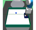
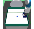
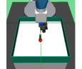
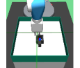
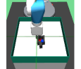
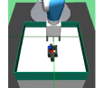
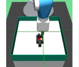
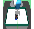
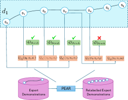
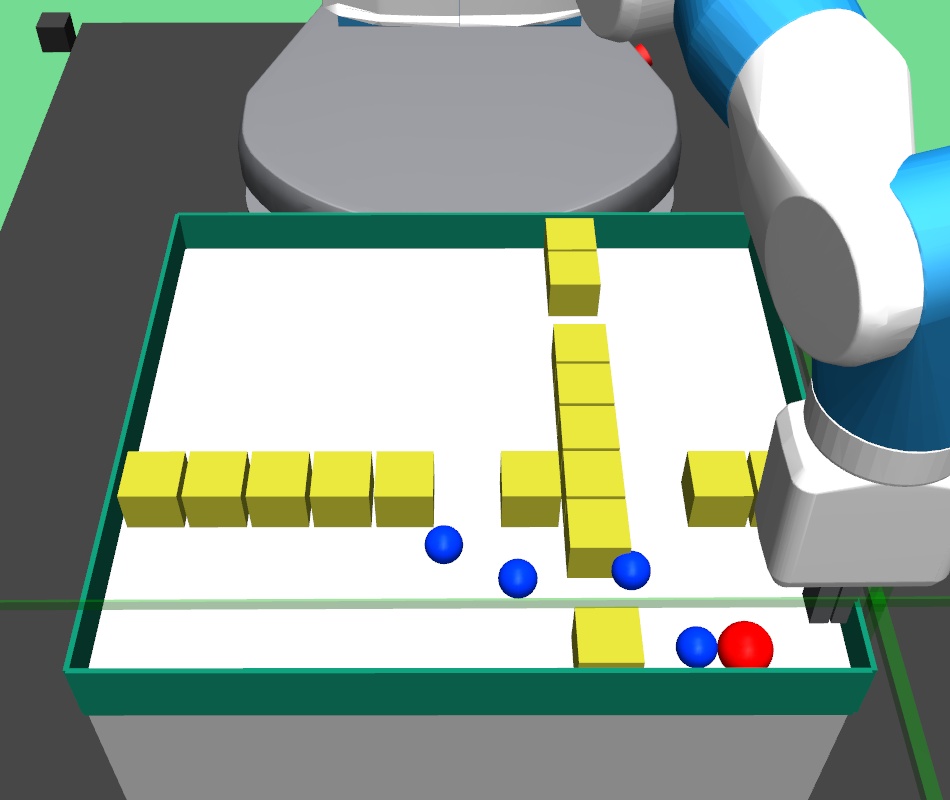
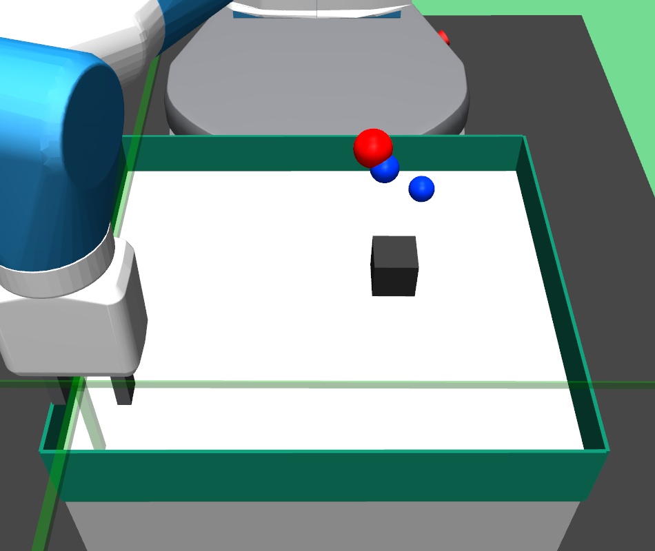
PEAR performs adaptive relabeling on expert demonstration trajectories to generate efficient higher level subgoal transition datatset , by employing the current lower primitive’s action value function . In a typical goal-conditioned RL setting, describes the expected cumulative reward where the start state and subgoal are and , and the lower primitive takes action while following policy . While parsing , we consecutively pass the expert demonstrations states as subgoals, and computes the expected cumulative reward when the start state is , subgoal is and the next primitive action is . Intuitively, a high value of implies that the current lower primitive considers to be a good (highly rewarding and achievable) subgoal from current state , since it expects to achieve a high intrinsic reward for this subgoal from the higher policy. Hence, considers goal achieving capability of current lower primitive for populating . We depict a single pass of adaptive relabeling in Figure 2 and explain the procedure in detail below.
Adaptive Relabeling Consider the demonstration dataset , where each trajectory . Let the initial state be . In the adaptive relabeling procedure, we incrementally provide demonstration states for to as subgoals to lower primitive’s action value function , where . At every step, we compare to a threshold ( works consistently for all experiments). If , we move on to next expert demonstration state . Otherwise, we consider to be a good subgoal (since it was the last subgoal with ), and use it to compute subgoal transitions for populating . Subsequently, we repeat the same procedure with as the new initial state, until the episode terminates. This is depicted in Figure 2 and Algorithm 1.
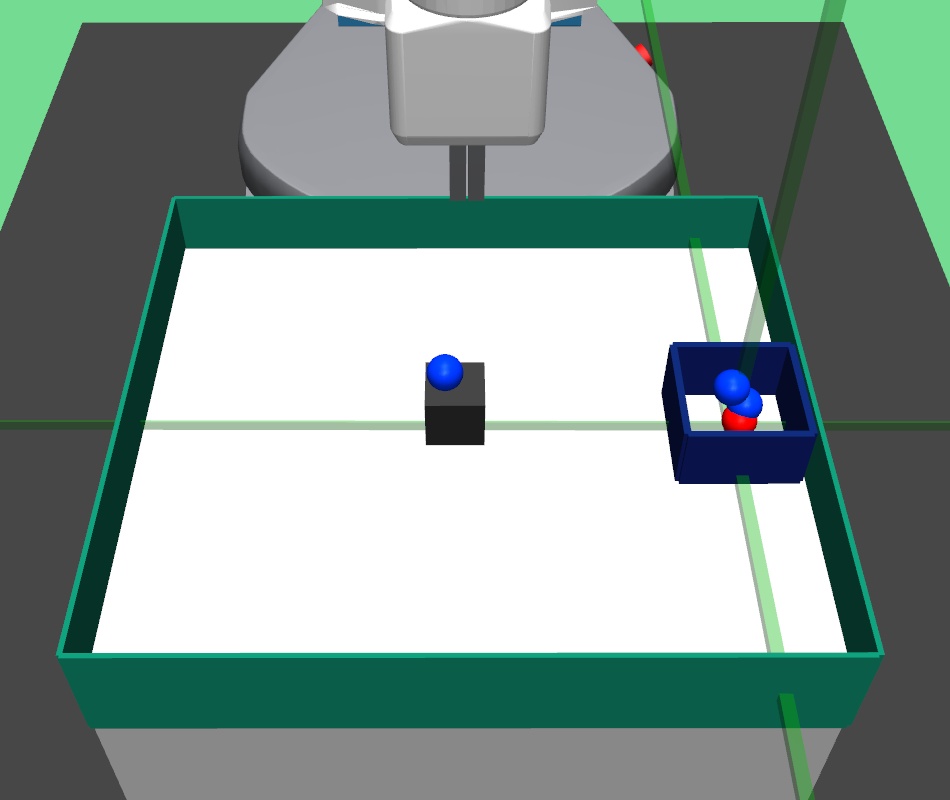
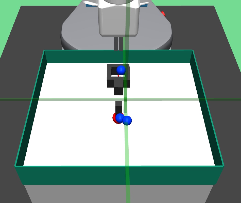
Periodic re-population of higher level subgoal dataset HRL approaches suffer from non-stationarity due to unstable higher level station transition and reward functions. In off-policy HRL, this occurs since previously collected experience is rendered obsolete due to continuously changing lower primitive. We propose to mitigate this non-stationarity by periodically re-populating subgoal transition dataset after every timesteps according to the goal achieving capability of the current lower primitive. Since the lower primitive continuously improves with training and gets better at achieving harder subgoals, always picks reachable subgoals of appropriate difficulty, according to the current lower primitive. This generates a natural curriculum of achievable subgoals for the lower primitive. Intuitively, always contains achievable subgoals for the current lower primitive, which mitigates non-stationarity in HRL. The pseudocode for PEAR is given in Algorithm 2. Figure 2 shows the qualitative evolution of subgoals with training in our experiments.
Dealing with out-of-distribution states Our adaptive relabeling procedure uses to select efficient subgoals when the expert state is within the training distribution of states used to train the lower primitive. However, if the expert states are outside the training distribution, might erroneously over-estimate the values on such states, which might result in poor subgoal selection. In order to address this over-estimation issue, we employ an additional margin classification objective(Piot et al., 2014), where along with the standard objective, we also use an additional margin classification objective to yield the following optimization objective
This surrogate objective prevents over-estimation of by penalizing states that are out of the expert state distribution. We found this objective to improve performance and stabilize learning. In the next section, we explain how we use adaptive relabeling to yield our joint optimization objective.
4.2 Joint optimization
Here, we explain our joint optimization objective that comprises of off-policy RL objective with IL based regularization, using generated using primitive enabled adaptive relabeling. We consider both behavior cloning (BC) and inverse reinforcement learning (IRL) regularization. Henceforth, PEAR-IRL will represent PEAR with IRL regularization and PEAR-BC will represent PEAR with BC regularization. We first explain BC regularization objective, and then explain IRL regularization objectives for both hierarchical levels.
For the BC objective, let represent a higher level subgoal transition from where is current state, is next state, is final goal and is subgoal supervision. Let be the subgoal predicted by the high level policy with parameters . The BC regularization objective for higher level is as follows:
| (1) | ||||
Similarly, let represent lower level expert transition where is current state, is next state, is goal and is the primitive action predicted by with parameters . The lower level BC regularization objective is as follows:
| (2) | ||||
We now consider the IRL objective, which is implemented as a GAIL (Ho and Ermon, 2016) objective implemented using LSGAN (Mao et al., 2016). Let be the higher level discriminator with parameters . Let represent higher level IRL objective, which depends on parameters . The higher level IRL regularization objective is as follows:
| (3) | ||||
Similarly, for lower level primitive, let be the lower level discriminator with parameters . Let represent lower level IRL objective, which depends on parameters . The lower level IRL regularization objective is as follows:
| (4) | ||||
Finally, we describe our joint optimization objective for hierarchical policies. Let the off-policy RL objective be and for higher and lower policies. The joint optimization objectives using BC regularization for higher and lower policies are provided in Equations 5 and 6 respectively.
| (5) |
| (6) |
The joint optimization objectives using IRL regularization for higher and lower policies are provided in Equations 7 and 8 respectively.
| (7) |
| (8) |
Here, is regularization weight hyper-parameter. We describe ablations to choose in Section 5.
4.3 Sub-optimality analysis
In this section, we perform theoretical analysis to derive sub-optimality bounds for our proposed joint optimization objective and show how our periodic re-population based approach affects performance, and propose a generalized framework for joint optimization using RL and IL. Let and be unknown higher level and lower level optimal policies. Let be our high level policy and be our lower primitive policy, where and are trainable parameters. denotes total variation divergence between probability distributions and . Let be an unknown distribution over states and actions, be goal space, be current state, and be the final episodic goal. We use in the importance sampling ratio later to avoid sampling from the unknown optimal policy (Appendix A.1). The higher level policy predicts subgoals for the lower primitive which is executed for timesteps to yield sub-trajectories . Let and be some unknown higher and lower level probability distributions over policies from which we can sample policies and . Let us assume that policies and represent the policies from higher and lower level datasets and respectively. Although and may represent any datasets, in our discussion, we use them to represent higher and lower level expert demonstration datasets. Firstly, we introduce the -common definition (Ajay et al., 2020) in goal-conditioned policies:
Definition 1.
is -common in , if
Now, we define the suboptimality of policy with respect to optimal policy as:
| (9) | ||||
Theorem 1.
Assuming optimal policy is common in , the suboptimality of higher policy , over length sub-trajectories sampled from can be bounded as:
| (10) | ||||
where
Similarly, the suboptimality of lower primitive can be bounded as:
| (11) | ||||
where
The proofs for Equations 10 and 11 are provided in Appendix A.1. We next discuss the effect of training on the two terms in RHS of Equation 10, which bound the suboptimality of .
Effect of adaptive relabeling on sub-optimality bounds We firstly focus on the first term which is dependent on . Since we represent the generated subgoal dataset as , we replace with . In Theorem 1, we assume the optimal policy to be common in . Since denotes the upper bound of the expected TV divergence between and , provides a quality measure of the subgoal dataset populated using adaptive relabeling. Intuitively, a lower value of implies that the optimal policy is closely represented by , or alternatively, the samples from are near optimal. As the lower primitive improves with training and is able to achieve harder subgoals, and since is re-populated using the improved lower primitive after every timesteps, continually gets closer to , which results in reduced value of . This implies that due to decreasing first term, the suboptimality bound in Equation 10 gets tighter, and consequently gets closer to optimal objective. Hence, our periodic re-population based approach generates a natural curriculum of achievable subgoals for the lower primitive, which continuously improves the performance by tightening the upper bound.
Effect of IL regularization on sub-optimality bounds Now, we focus on the second term in Equation 10, which is TV divergence between and with expectation over . As before, is replaced by dataset . This term can be viewed as imitation learning (IL) objective between expert demonstration policy and current policy , where TV divergence is the distance measure. Due to this IL regularization objective, as policy gets closer to expert distribution policy with training, the LHS sub-optimality bounds get tighter. Thus, our proposed periodic IL regularization using tightens the sub-optimality bounds in Equation 10 with training, thereby improving performance.
Generalized framework We now derive our generalized framework for the joint optimization objective, where we can plug in off-the-shelf RL and IL methods to yield a generally applicable practical HRL algorithm. Considering sub-optimality is positive (Equation 9), we can use Equation 10 to derive the following objective:
| (12) | ||||
where (considering as , and as ), .
Notably, the second term in RHS of Equation 12 is constant for a given dataset . Equation 12 can be perceived as a minorize maximize algorithm which intuitively means: the overall objective can be optimized by maximizing the objective via RL, and minimizing the distance measure between and (IL regularization). This formulation serves as a framework where we can plug in RL algorithm of choice for off-policy RL objective , and distance function of choice for IL regularization, to yield various joint optimization objectives.
In our setup, we plug in entropy regularized Soft Actor Critic (Haarnoja et al., 2018a) to maximize . Notably, different parameterizations of yield different imitation learning regularizers. When is formulated as Kullback–Leibler divergence, the IL regularizer takes the form of behavior cloning (BC) objective (Nair et al., 2018) (which results in PEAR-BC), and when is formulated as Jensen-Shannon divergence, the imitation learning objective takes the form of inverse reinforcement learning (IRL) objective (which results in PEAR-IRL). We consider both these objectives in Section 5 and provide empirical performance results.
5 Experiments
In this section, we empirically answer the following questions: does adaptive relabeling approach outperform fixed relabeling based approaches, is PEAR able to mitigate non-stationarity, does IL regularization boost performance in solving complex long horizon tasks, and What is the contribution of each of our design choices? We accordingly perform experiments on six Mujoco (Todorov et al., 2012) environments: maze navigation, pick and place, bin, hollow, rope manipulation, and franka kitchen. Please refer to the supplementary for a video depicting qualitative results, and the implementation code.
Environment and Implementation Details: We provide extensive environment and implementation details, including number and procedure of collecting demonstrations in Appendix A.3. Since the environments are sparsely rewarded, they are complex tasks where the agent must explore the environment extensively before receiving any rewards. Unless otherwise stated, we keep the training conditions consistent across all baselines to ascertain fair comparisons, and empirically tune the hyper-parameter values of our method and all other baselines.

5.1 Evaluation and Results
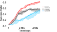
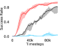
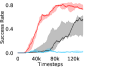
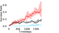
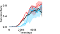
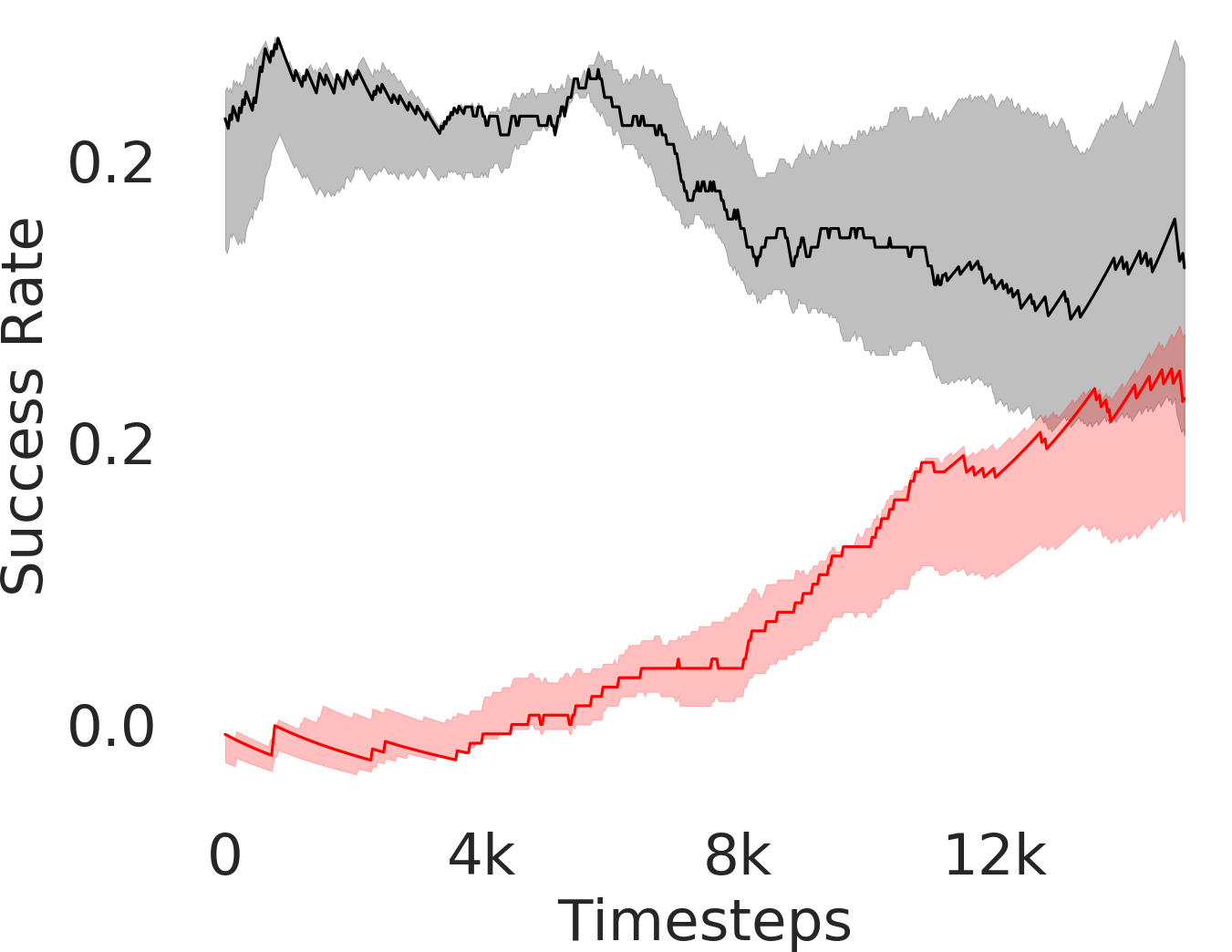
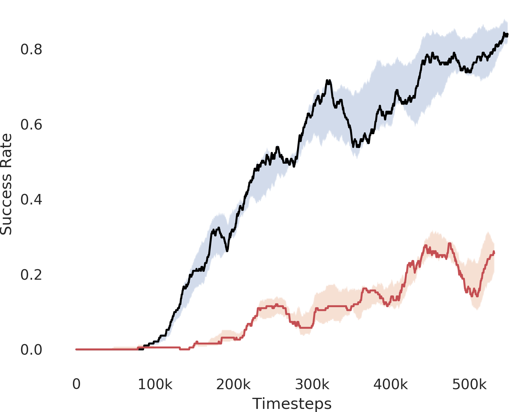
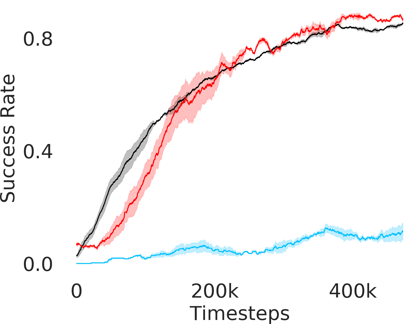
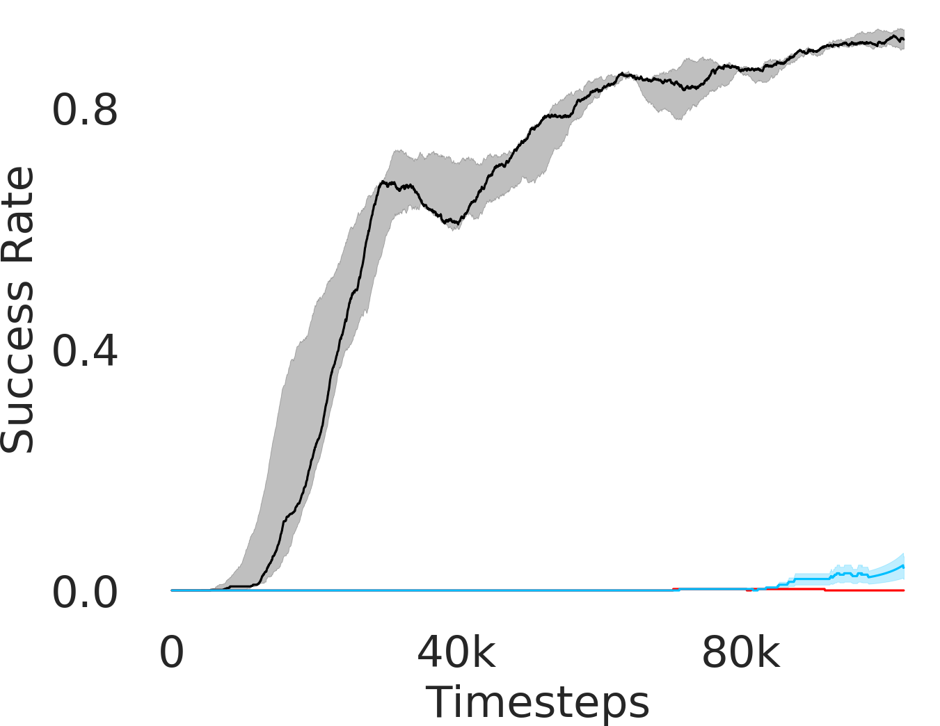
In Figure 3, we depict the success rate performance of PEAR and compare it with other baselines averaged over seeds. The primary goal of these comparisons is to verify that the proposed approach indeed mitigates non-stationarity and demonstrates improved performance and training stability.
Comparing with fixed window based approach
RPL: In order to demonstrate the efficacy of adaptive relabeling, we compare our method with Relay Policy Learning (RPL) baseline. RPL (Gupta et al., 2019) uses supervised pre-training followed by relay fine tuning. In order to ascertain fair comparisons, we use an ablation of RPL which does not use supervised pre-training. PEAR outperforms this baseline, which demonstrates that adaptive relabeling outperforms fixed window based relabeling and is crucial for mitigating non-stationarity. Since PEAR and RPL both employ jointly optimizing RL and IL based learning and only differ in adaptive relabeling, it is evident that adaptive relabeling is crucial for generating feasible subgoals.
Comparing with hierarchical baselines
RAPS: RAPS (Dalal et al., 2021) uses hand designed action primitives at the lower level, where the goal of the upper level is to pick the optimal sequence of action primitives. The performance of such approaches significantly depends on the quality of action primitives, which require substantial effort to hand-design. We found that except maze navigation task, RAPS is unable to perform well on other tasks, which we believe is because selecting appropriate primitive sequences is hard on other harder tasks. Notably, hand designing action primitives is exceptionally complex in environments like rope manipulation. Hence, we do not evaluate RAPS in rope environment.
HAC: Hierarchical actor critic (HAC) (Levy et al., 2018) deals with non-stationarity by relabeling transitions while assuming an optimal lower primitive. Although HAC shows good performance in maze navigation task, PEAR consistently outperforms HAC on all other tasks.
HIER-NEG and HIER: We also compare PEAR with two hierarchical baselines: HIER and HIER-NEG, which are hierarchical baselines that do not leverage expert demonstrations. HIER-NEG is a hierarchical baseline where the upper level is negatively rewarded if the lower primitive fails to achieve the subgoal. Since HIER, HIER-NEG and PEAR all are hierarchical approaches, we use these baseline comparisons to motivate that the performance improvement is not just due to use of hierarchical abstraction, but instead due to adaptive relabeling and primitive-enabled regularization. This is clearly evidenced by superior performance of PEAR.
Comparing with non-hierarchical baselines
Additionally, we consider single-level Discriminator Actor Critic (DAC) (Kostrikov et al., 2019) that leverages expert demos, single-level SAC (FLAT) baseline, and Behavior Cloning (BC) baselines. However, they fail to perform well in any of the tasks.
5.2 Ablative analysis
Here, we perform ablation analysis to elucidate the significance of our design choices. We choose the hyper-parameter values after extensive experiments, and keep them consistent across all baselines.
Dealing with non-stationarity and infeasible subgoal generation in HRL:
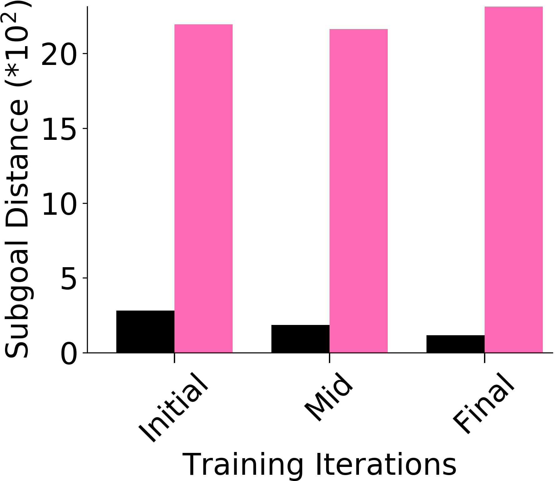
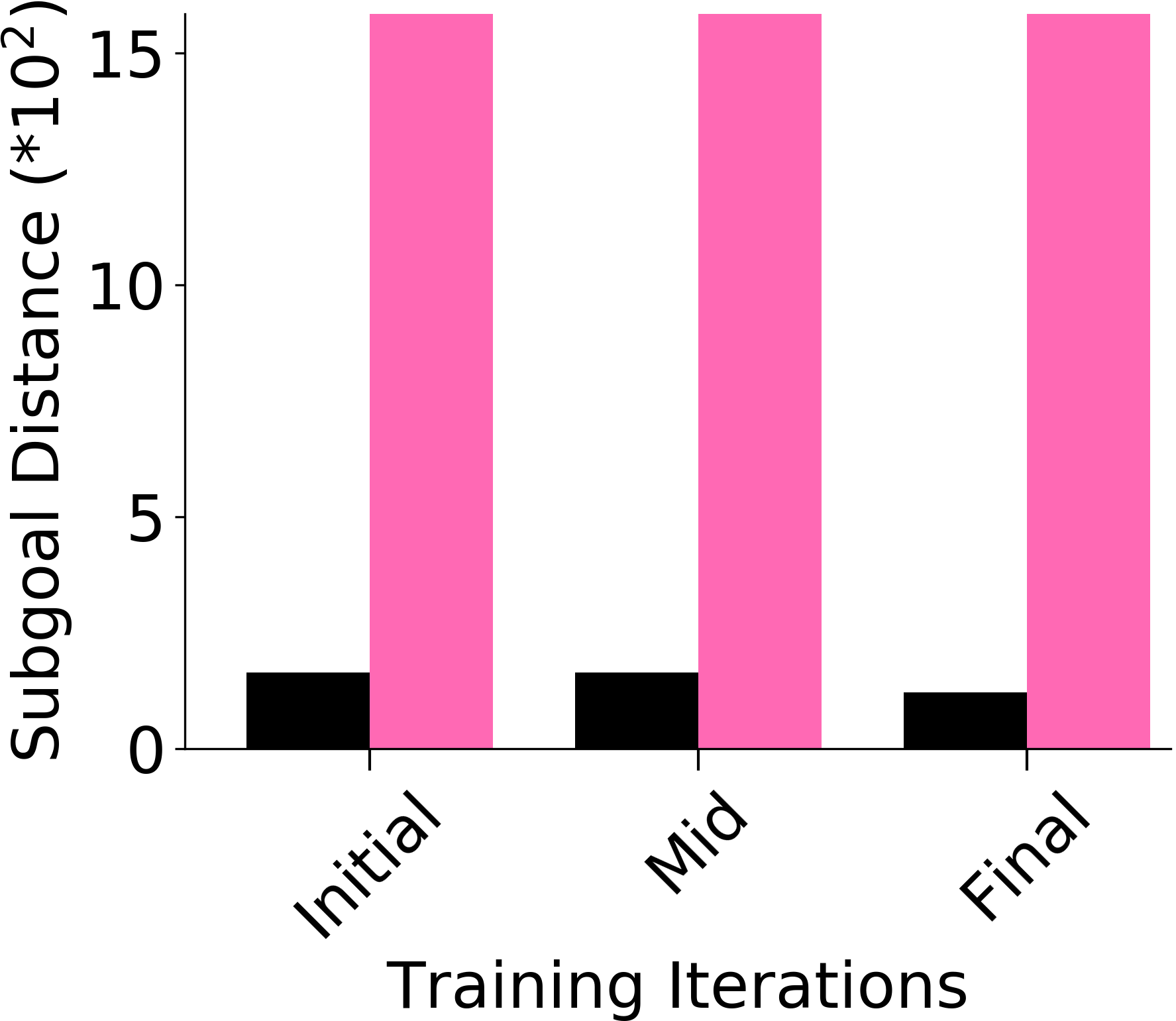
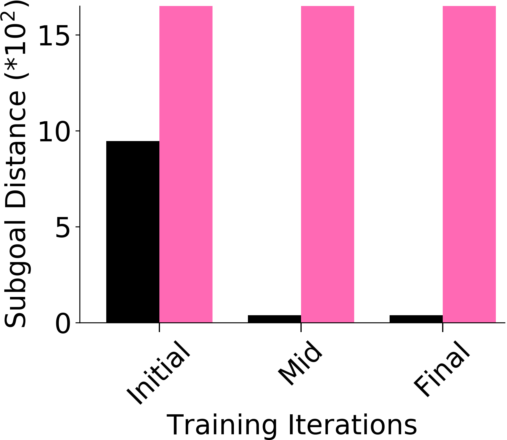
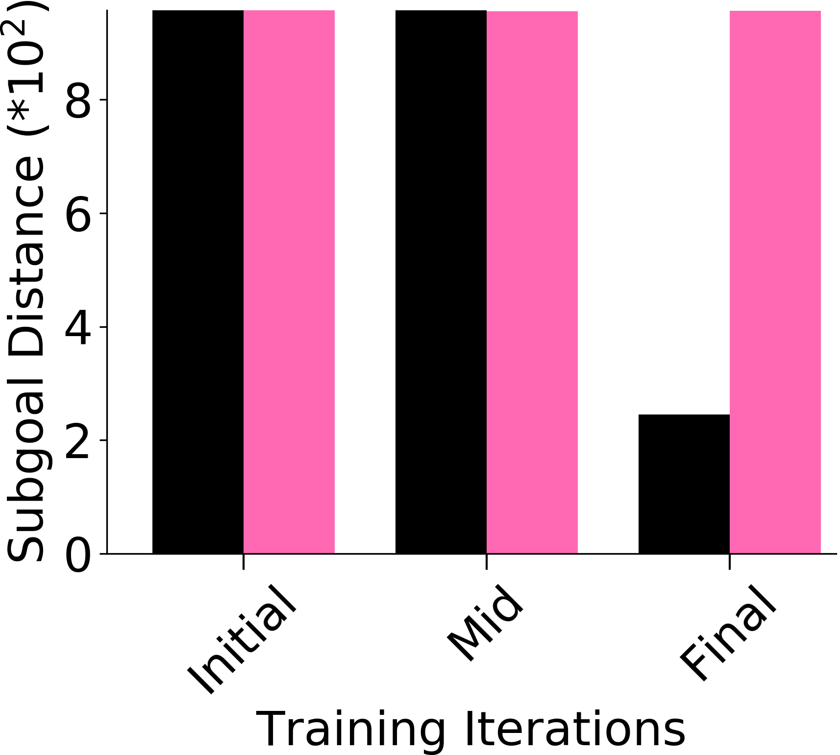
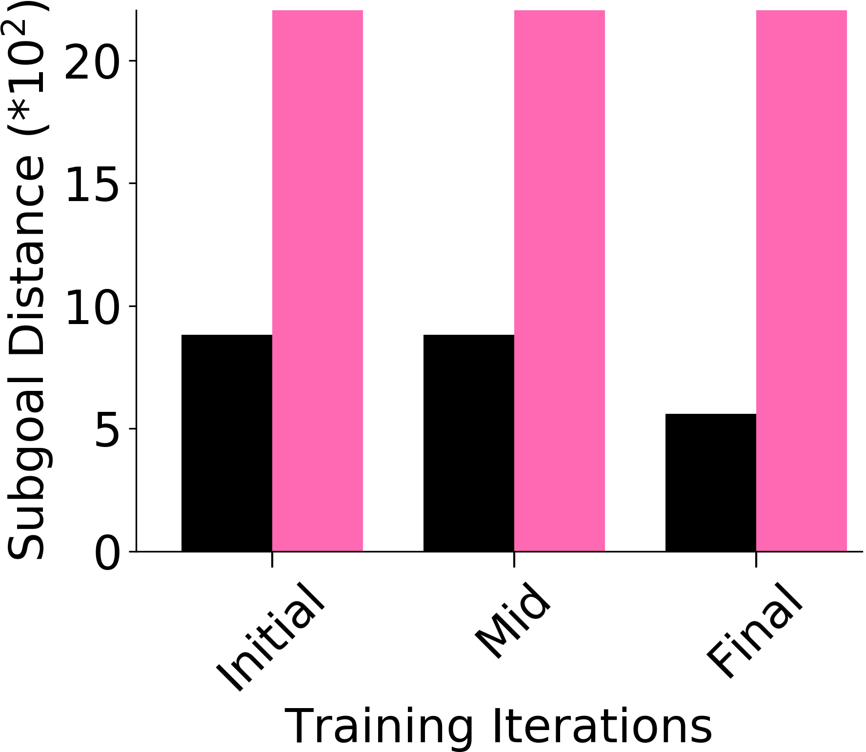
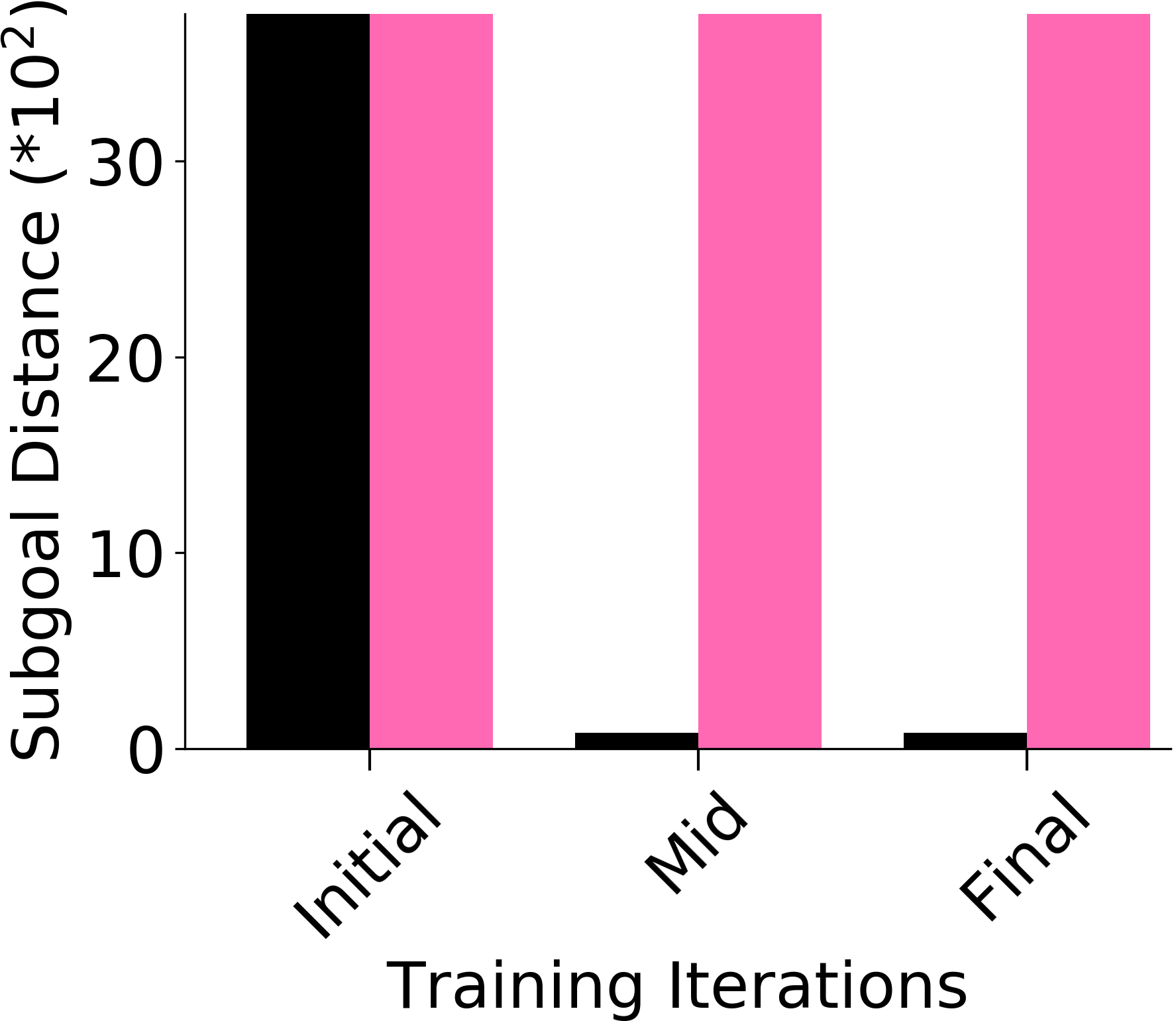

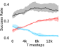
We assess whether PEAR mitigates non-stationarity in HRL by comparing it with the vanilla HIER baseline, as shown in Figure 4. We compute the average distance between subgoals predicted by the higher-level policy and those achieved by the lower-level primitive throughout training. A lower average distance suggests that PEAR generates subgoals achievable by the lower primitive, inducing lower primitive behavior to be optimal. Our findings reveal that PEAR consistently maintains low average distances, validating its effectiveness in reducing non-stationarity. Additionally, as seen in Figure 4, post-training results show that PEAR achieves significantly lower distance values than the HIER baseline, highlighting its ability to generate feasible subgoals through primitive regularization.


Additional Ablations: First, we verify the importance of adaptive relabeling by replacing it in PEAR-IRL by fixed window relabeling (as in RPL (Gupta et al., 2019)). As seen in Figure 6, this ablation (PEAR-IRL) consistently outperforms PEAR-RPL on all tasks, which demonstrates the benefit of adaptive relabeling. Further, we compare PEAR-IRL and PEAR-BC (with margin classification objectives), with PEAR-IRL-No-Margin and PEAR-BC-No-Margin (without margin objectives) in Figure 7. PEAR-IRL and PEAR-BC outperform their No-Margin counterparts, which shows that this objective efficiently deals with the issue of out-of-distribution states, and induces training stability.
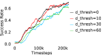
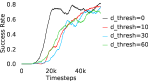
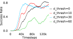
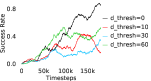
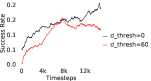
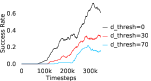
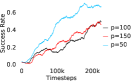
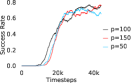
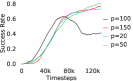
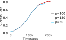
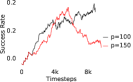
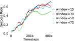
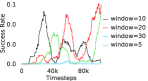
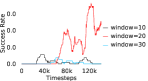
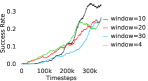
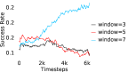
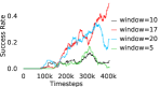
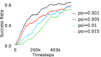
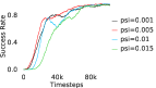
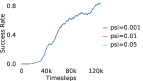
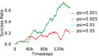
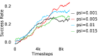
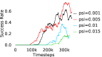
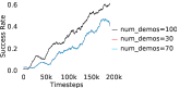
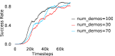
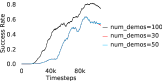
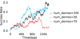
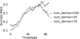
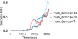
Further, we analyse how varying affects performance in Appendix A.4 Figure 8. We next study the impact of varying . Intuitively, if is too large, it impedes generation of a good curriculum of subgoals (Appendix A.4 Figure 9). Also, a low value of may lead to frequent subgoal dataset re-population and may impede stable learning. We also choose optimal window size for RPL experiments, as shown in Appendix A.4 Figure 10. We also evaluate learning rate in Appendix A.4 Figure 11. If is too small, PEAR is unable to utilize IL regularization, whereas conversely if is too large, the learned policy might overfit. We also deduce the optimal number of expert demonstrations required in Appendix A.4 Figure 12. Next, we compare the performance of PEAR-IRL with HER-BC, which is a single-level implementation of HER with expert demonstrations. As seen in Appendix A.4 Figure 13, PEAR significantly outperforms this baseline, which demonstrates the advantage of our hierarchical formulation. We also provide qualitative visualizations in Appendix A.5.
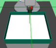
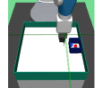
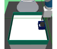
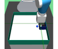
Real world experiments: We perform experiments on real world robotic pick and place, bin and rope environments (Fig 6). We use Realsense D435 depth camera to extract the robotic arm position, block, bin, and rope cylinder positions. Computing accurate linear and angular velocities is hard in real tasks, so we assign them small hard-coded values, which shows good performance. We performed sets of experiments with trial each, and report the average success rates. PEAR-IRL achieves accuracy of , , and , whereas PEAR-BC achieves accuracy of , , on pick and place, bin and rope environments. We also evaluate the performance of next best performing RPL baseline, but it fails to achieve success in any of the tasks.
6 Discussion
Limitations In this work, we assume availability of directed expert demonstrations, which we plan to deal with in future. Additionally, is periodically re-populated, which is an additional overhead and might be a bottleneck in tasks where relabeling cost is high. Notably, we side-step this limitation by passing the whole expert trajectory as a mini-batch for a single forward pass through lower primitive. Nevertheless, we plan to deal with these limitations in future work.
Conclusion and future work We propose primitive enabled adaptive relabeling (PEAR), a HRL and IL based approach that performs adaptive relabeling on a few expert demonstrations to solve complex long horizon tasks. We perform comparisons with a various baselines and demonstrate that PEAR shows strong results in simulation and real world robotic tasks. In future work, we plan to address harder sequential decision making tasks, and plan to analyse generalization beyond expert demonstrations. We hope that PEAR encourages future research in the area of adaptive relabeling and primitive informed regularization, and leads to efficient approaches to solve long horizon tasks.
References
- Ajay et al. [2020] Anurag Ajay, Aviral Kumar, Pulkit Agrawal, Sergey Levine, and Ofir Nachum. Opal: Offline primitive discovery for accelerating offline reinforcement learning. In Advances in Neural Information Processing Systems (NeurIPS), pages 1–12. Curran Associates Inc., 2020. URL https://proceedings.neurips.cc/paper/2020/file/1f1b5c3b8f1b5c3b8f1b5c3b8f1b5c3b-Paper.pdf.
- Andrychowicz et al. [2017] Marcin Andrychowicz, Filip Wolski, Alex Ray, Jonas Schneider, Rachel Fong, Peter Welinder, Bob McGrew, Josh Tobin, OpenAI Pieter Abbeel, and Wojciech Zaremba. Hindsight experience replay. Advances in neural information processing systems, 30, 2017.
- Bacon et al. [2017] Pierre-Luc Bacon, Jean Harb, and Doina Precup. The option-critic architecture. In Proceedings of the AAAI conference on artificial intelligence, volume 31, 2017.
- Barto and Mahadevan [2003] Andrew G Barto and Sridhar Mahadevan. Recent advances in hierarchical reinforcement learning. Discrete Event Dynamic Systems, 13(4):341–379, 2003.
- Chane-Sane et al. [2021] Elliot Chane-Sane, Cordelia Schmid, and Ivan Laptev. Goal-conditioned reinforcement learning with imagined subgoals. In Proceedings of Advances in Neural Information Processing Systems (NeurIPS), page TBD, 2021.
- Dalal et al. [2021] Murtaza Dalal, Deepak Pathak, and Ruslan Salakhutdinov. Accelerating robotic reinforcement learning via parameterized action primitives. In Advances in Neural Information Processing Systems (NeurIPS), 2021. URL https://arxiv.org/abs/2110.15360.
- Dayan and Hinton [1993] Peter Dayan and Geoffrey E Hinton. Feudal reinforcement learning. In Advances in Neural Information Processing Systems, pages 271–278. Morgan Kaufmann Publishers Inc., 1993.
- Dietterich [2000] Thomas G. Dietterich. Hierarchical reinforcement learning with the maxq value function decomposition. Journal of Artificial Intelligence Research, 13:227–303, 2000. URL https://www.jair.org/index.php/jair/article/view/10266.
- Ding et al. [2019] Yiming Ding, Carlos Florensa, Pieter Abbeel, and Mariano Phielipp. Goal-conditioned imitation learning. In Advances in Neural Information Processing Systems (NeurIPS), 2019.
- Foster and Dayan [2002] David Foster and Peter Dayan. Structure in the space of value functions. Machine Learning, 49(2–3):325–346, 2002.
- Fox et al. [2017] Roy Fox, Sanjay Krishnan, Ion Stoica, and Ken Goldberg. Multi-level discovery of deep options. In Proceedings of the 34th International Conference on Machine Learning (ICML), pages 1665–1674. PMLR, 2017. URL https://proceedings.mlr.press/v70/fox17a.html.
- Fu et al. [2020] Justin Fu, Aviral Kumar, Ofir Nachum, George Tucker, and Sergey Levine. D4rl: Datasets for deep data-driven reinforcement learning. In Conference on Robot Learning (CoRL), pages 729–735. PMLR, 2020.
- Gu et al. [2017] Shixiang Gu, Ethan Holly, Timothy Lillicrap, and Sergey Levine. Deep reinforcement learning for robotic manipulation with asynchronous off-policy updates. In 2017 IEEE International Conference on Robotics and Automation (ICRA), pages 3389–3396. IEEE, 2017. doi: 10.1109/ICRA.2017.7989385. URL https://ieeexplore.ieee.org/document/7989385.
- Gupta et al. [2019] Abhishek Gupta, Vikash Kumar, Corey Lynch, Sergey Levine, and Karol Hausman. Relay policy learning: Solving long horizon tasks via imitation and reinforcement learning. In Conference on Robot Learning (CoRL), 2019.
- Haarnoja et al. [2018a] Tuomas Haarnoja, Kristian Hartikainen, Pieter Abbeel, and Sergey Levine. Latent space policies for hierarchical reinforcement learning. In International Conference on Machine Learning, pages 1851–1860. PMLR, 2018a.
- Haarnoja et al. [2018b] Tuomas Haarnoja, Aurick Zhou, Pieter Abbeel, and Sergey Levine. Soft actor-critic: Off-policy maximum entropy deep reinforcement learning with a stochastic actor. In Proceedings of the 35th International Conference on Machine Learning (ICML), pages 1861–1870. PMLR, 2018b. URL https://proceedings.mlr.press/v80/haarnoja18b.html.
- Harb et al. [2018] Jean Harb, Pierre-Luc Bacon, Martin Klissarov, and Doina Precup. When waiting is not an option: Learning options with a deliberation cost. In Proceedings of the 32nd AAAI Conference on Artificial Intelligence (AAAI), pages 3206–3213, 2018. URL https://ojs.aaai.org/index.php/AAAI/article/view/11741.
- Harutyunyan et al. [2018] Anna Harutyunyan, Peter Vrancx, Pierre-Luc Bacon, Doina Precup, and Ann Nowé. Learning with options that terminate off-policy. In Proceedings of the 32nd AAAI Conference on Artificial Intelligence (AAAI), pages 3201–3208, 2018. URL https://ojs.aaai.org/index.php/AAAI/article/view/11740.
- Harutyunyan et al. [2019] Anna Harutyunyan, Will Dabney, Diana Borsa, Nicolas Heess, Rémi Munos, and Doina Precup. The termination critic. In Proceedings of the 36th International Conference on Machine Learning (ICML), pages 2645–2653, 2019. URL http://proceedings.mlr.press/v97/harutyunyan19a.html.
- Hester et al. [2018] Todd Hester, Matej Vecerik, Olivier Pietquin, Marc Lanctot, Tom Schaul, Bilal Piot, Andrew Sendonaris, Gabriel Dulac-Arnold, Ian Osband, John P. Agapiou, Joel Z. Leibo, and Audrunas Gruslys. Deep q-learning from demonstrations. In Proceedings of the Thirty-Second AAAI Conference on Artificial Intelligence (AAAI), pages 3223–3230, 2018. URL https://ojs.aaai.org/index.php/AAAI/article/view/11794.
- Ho and Ermon [2016] Jonathan Ho and Stefano Ermon. Generative adversarial imitation learning. In Advances in Neural Information Processing Systems (NeurIPS), pages 4565–4573, 2016. URL https://proceedings.neurips.cc/paper/2016/hash/cc7e2b878868cbae992d1fb743995d8f-Abstract.html.
- Kaelbling [1993] Leslie Pack Kaelbling. Learning to achieve goals. In Proceedings of the International Joint Conference on Artificial Intelligence (IJCAI), pages 1094–1098, 1993.
- Kalashnikov et al. [2018] Dmitry Kalashnikov, Alex Irpan, Peter Pastor, Julian Ibarz, Alexander Herzog, Eric Jang, Deirdre Quillen, Ethan Holly, Mrinal Kalakrishnan, Vincent Vanhoucke, et al. Scalable deep reinforcement learning for vision-based robotic manipulation. In Conference on robot learning, pages 651–673. PMLR, 2018.
- Kipf et al. [2019] Thomas Kipf, Yujia Li, Hanjun Dai, Vinicius Zambaldi, Alvaro Sanchez-Gonzalez, Edward Grefenstette, Pushmeet Kohli, and Peter Battaglia. Compile: Compositional imitation learning and execution. In International Conference on Machine Learning, pages 3418–3428. PMLR, 2019.
- Klissarov et al. [2017] Martin Klissarov, Pierre-Luc Bacon, Jean Harb, and Doina Precup. Learning options end-to-end for continuous action tasks. In Proceedings of the 31st Conference on Neural Information Processing Systems (NeurIPS) Hierarchical Reinforcement Learning Workshop, 2017. URL https://arxiv.org/abs/1712.00004.
- Kostrikov et al. [2019] Ilya Kostrikov, Kumar Krishna Agrawal, Debidatta Dwibedi, Sergey Levine, and Jonathan Tompson. Discriminator-actor-critic: Addressing sample inefficiency and reward bias in adversarial imitation learning. In 7th International Conference on Learning Representations (ICLR), 2019. URL https://openreview.net/forum?id=Hk4fpoA5Km.
- Kreidieh et al. [2020] Abdul Rahman Kreidieh, Samyak Parajuli, Nathan Lichtlé, Yiling You, Rayyan Nasr, and Alexandre M. Bayen. Inter-level cooperation in hierarchical reinforcement learning. In Proceedings of the 19th International Conference on Autonomous Agents and MultiAgent Systems (AAMAS), pages 2000–2002, 2020. URL https://dl.acm.org/doi/10.5555/3398761.3398990.
- Krishnan et al. [2017] Sanjay Krishnan, Roy Fox, Ion Stoica, and Ken Goldberg. DDCO: Discovery of deep continuous options for robot learning from demonstrations. In Proceedings of the 1st Annual Conference on Robot Learning (CoRL), pages 418–437, 2017. URL https://proceedings.mlr.press/v78/krishnan17a.html.
- Krishnan et al. [2019] Sanjay Krishnan, Animesh Garg, Richard Liaw, Brijen Thananjeyan, Lauren Miller, Florian T. Pokorny, and Ken Goldberg. Swirl: A sequential windowed inverse reinforcement learning algorithm for robot tasks with delayed rewards. The International Journal of Robotics Research, 38(2-3):126–145, 2019. doi: 10.1177/0278364918784350. URL https://doi.org/10.1177/0278364918784350.
- LaValle [1998] Steven M LaValle. Rapidly-exploring random trees: A new tool for path planning. Technical report, Tech. rep., 1998.
- Lee et al. [2023] Seungjae Lee, Jigang Kim, Inkyu Jang, and H. Jin Kim. Dhrl: A graph-based approach for long-horizon and sparse hierarchical reinforcement learning. In Proceedings of the IEEE International Conference on Robotics and Automation (ICRA), page TBD. IEEE, 2023.
- Levine et al. [2016] Sergey Levine, Chelsea Finn, Trevor Darrell, and Pieter Abbeel. End-to-end training of deep visuomotor policies. Journal of Machine Learning Research, 17(39):1–40, 2016.
- Levy et al. [2018] Andrew Levy, Robert Platt, and Kate Saenko. Hierarchical actor-critic. In Proceedings of the 6th International Conference on Learning Representations (ICLR), 2018. URL https://openreview.net/forum?id=SJ3rcZ0cK7.
- Mao et al. [2016] Xudong Mao, Qing Li, Haoran Xie, Raymond YK Lau, and Zhen Wang. Multi-class generative adversarial networks with the l2 loss function. arXiv preprint arXiv:1611.04076, 5:1057–7149, 2016.
- Nachum et al. [2018] Ofir Nachum, Shixiang Gu, Honglak Lee, and Sergey Levine. Data-efficient hierarchical reinforcement learning. In Advances in Neural Information Processing Systems, volume 31, pages 3303–3313, 2018. URL https://proceedings.neurips.cc/paper/2018/hash/e6384711491713d29bc63fc5eeb5ba4f-Abstract.html.
- Nachum et al. [2019] Ofir Nachum, Haoran Tang, Xingyu Lu, Shixiang Gu, Honglak Lee, and Sergey Levine. Why does hierarchy (sometimes) work so well in reinforcement learning? In Proceedings of the 33rd Conference on Neural Information Processing Systems (NeurIPS), 2019. URL https://arxiv.org/abs/1909.10618.
- Nair et al. [2018] Ashvin Nair, Bob McGrew, Marcin Andrychowicz, Wojciech Zaremba, and Pieter Abbeel. Overcoming exploration in reinforcement learning with demonstrations. In 2018 IEEE International Conference on Robotics and Automation (ICRA), pages 6292–6299. IEEE, 2018. doi: 10.1109/ICRA.2018.8463162. URL https://ieeexplore.ieee.org/document/8463162.
- Nasiriany et al. [2022] Soroush Nasiriany, Huihan Liu, and Yuke Zhu. Augmenting reinforcement learning with behavior primitives for diverse manipulation tasks. In IEEE International Conference on Robotics and Automation (ICRA), pages 7477–7484, 2022. URL https://arxiv.org/abs/2110.03655.
- Parr and Russell [1998] Ronald Parr and Stuart Russell. Reinforcement learning with hierarchies of machines. In Advances in Neural Information Processing Systems 10. MIT Press, 1998.
- Pertsch et al. [2020] Karl Pertsch, Youngwoon Lee, and Joseph J. Lim. Accelerating reinforcement learning with learned skill priors. In Conference on Robot Learning (CoRL), pages 944–957, 2020. URL https://arxiv.org/abs/2010.11944.
- Piot et al. [2014] Bilal Piot, Matthieu Geist, and Olivier Pietquin. Boosted bellman residual minimization handling expert demonstrations. In European Conference on Machine Learning and Principles and Practice of Knowledge Discovery in Databases (ECML/PKDD), 2014.
- Rajeswaran et al. [2018] Aravind Rajeswaran, Vikash Kumar, Abhishek Gupta, Giulia Vezzani, John Schulman, Emanuel Todorov, and Sergey Levine. Learning complex dexterous manipulation with deep reinforcement learning and demonstrations. In Proceedings of Robotics: Science and Systems (RSS). Robotics: Science and Systems Foundation, 2018.
- Salter et al. [2022a] Sasha Salter, Kristian Hartikainen, Walter Goodwin, and Ingmar Posner. Priors, hierarchy, and information asymmetry for skill transfer in reinforcement learning. In Proceedings of the 5th Conference on Robot Learning (CoRL), page TBD. PMLR, 2022a.
- Salter et al. [2022b] Sasha Salter, Markus Wulfmeier, Dhruva Tirumala, et al. Mo2: Model-based offline options. In Conference on Lifelong Learning Agents, pages 902–919, 2022b.
- Schaul et al. [2015] Tom Schaul, Daniel Horgan, Karol Gregor, and David Silver. Universal value function approximators. In Francis Bach and David Blei, editors, Proceedings of the 32nd International Conference on Machine Learning, volume 37 of Proceedings of Machine Learning Research, pages 1312–1320, Lille, France, 2015. PMLR. URL https://proceedings.mlr.press/v37/schaul15.html.
- Shiarlis et al. [2018] Konstantinos Shiarlis, Markus Wulfmeier, Shaun Salter, Shimon Whiteson, and Ingmar Posner. Taco: Learning task decomposition via temporal alignment for control. In Proceedings of the 35th International Conference on Machine Learning, pages 4654–4663. PMLR, 2018.
- Singh et al. [2021] Avi Singh, Huihan Liu, Gaoyue Zhou, Tianhe Yu, Pieter Abbeel, Chelsea Finn, and Sergey Levine. Parrot: Data-driven behavioral priors for reinforcement learning. In 9th International Conference on Learning Representations (ICLR), 2021. URL https://arxiv.org/abs/2011.10024.
- Sutton et al. [1999] Richard S Sutton, Doina Precup, and Satinder Singh. Between mdps and semi-mdps: A framework for temporal abstraction in reinforcement learning. Artificial intelligence, 112(1-2):181–211, 1999.
- Tirumala et al. [2022] Dhruva Tirumala, Alexandre Galashov, et al. Behavior priors for efficient reinforcement learning. Journal of Machine Learning Research, 23(221):1–68, 2022.
- Todorov et al. [2012] Emanuel Todorov, Tom Erez, and Yuval Tassa. Mujoco: A physics engine for model-based control. In 2012 IEEE/RSJ International Conference on Intelligent Robots and Systems, pages 5026–5033. IEEE, 2012.
- Vezhnevets et al. [2017] Alexander Sasha Vezhnevets, Simon Osindero, Tom Schaul, Nicolas Heess, Max Jaderberg, David Silver, and Koray Kavukcuoglu. Feudal networks for hierarchical reinforcement learning. In International conference on machine learning, pages 3540–3549. PMLR, 2017.
- Wulfmeier et al. [2019] Markus Wulfmeier, Abbas Abdolmaleki, Roland Hafner, Jost Tobias Springenberg, et al. Regularized hierarchical policies for compositional transfer in robotics. arXiv preprint arXiv:1906.11228, 2019.
- Wulfmeier et al. [2021] Markus Wulfmeier, Dushyant Rao, Roland Hafner, et al. Data-efficient hindsight off-policy option learning. In International Conference on Machine Learning (ICML), pages 11340–11350, 2021.
- Zhang et al. [2020] Tianren Zhang, Shangqi Guo, Tian Tan, Xiaolin Hu, and Feng Chen. Generating adjacency-constrained subgoals in hierarchical reinforcement learning. In Advances in Neural Information Processing Systems, volume 33, pages 9814–9826, 2020. URL https://proceedings.neurips.cc/paper/2020/file/f5f3b8d720f34ebebceb7765e447268b-Paper.pdf.
Appendix A Appendix
A.1 Sub-optimality analysis
Here, we present the proofs for Theorem 1 for higher and lower level policies, which provide sub-optimality bounds on the optimization objectives.
A.1.1 Sub-optimality proof for higher level policy
The sub-optimality of upper policy , over length sub-trajectories sampled from can be bounded as:
| (13) | ||||
where
Proof.
We extend the suboptimality bound from [Ajay et al., 2020] between goal conditioned policies and as follows:
| (14) | ||||
By applying triangle inequality:
| (15) | ||||
Taking expectation wrt , and ,
| (16) | ||||
Since is common in , we can write 16 as:
| (17) | ||||
Substituting the result from align 17 in align 14, we get
| (18) | ||||
where ∎
A.1.2 Sub-optimality proof for lower level policy
Let the optimal lower level policy be . The suboptimality of lower primitive can be bounded as follows:
| (19) | ||||
where
Proof.
We extend the suboptimality bound from [Ajay et al., 2020] between goal conditioned policies and as follows:
| (20) | ||||
By applying triangle inequality:
| (21) | ||||
Taking expectation wrt , and ,
| (22) | ||||
Since is common in , we can write 22 as:
| (23) | ||||
Substituting the result from align 23 in align 20, we get
| (24) | ||||
where ∎
A.2 Generating expert demonstrations
For maze navigation, we use path planning RRT [LaValle, 1998] algorithm to generate expert demonstration trajectories. For pick and place, we hard coded an optimal trajectory generation policy for generating demonstrations, although they can also be generated using Mujoco VR [Todorov et al., 2012]. For kitchen task, the expert demonstrations are collected using Puppet Mujoco VR system [Fu et al., 2020]. In rope manipulation task, expert demonstrations are generated by repeatedly finding the closest corresponding rope elements from the current rope configuration and final goal rope configuration, and performing consecutive pokes of a fixed small length on the rope element in the direction of the goal configuration element. The detailed procedure are as follows:
A.2.1 Maze navigation task
We use the path planning RRT [LaValle, 1998] algorithm to generate optimal paths from the current state to the goal state. RRT has privileged information about the obstacle position which is provided to the methods through state. Using these expert paths, we generate state-action expert demonstration dataset for the lower level policy.
A.2.2 Pick and place task
In order to generate expert demonstrations, we can either use a human expert to perform the pick and place task in virtual reality based Mujoco simulation, or hard code a control policy. We hard-coded the expert demonstrations in our setup. In this task, the robot firstly picks up the block using robotic gripper, and then takes it to the target goal position. Using these expert trajectories, we generate expert demonstration dataset for the lower level policy.
A.2.3 Bin task
In order to generate expert demonstrations, we can either use a human expert to perform the bin task in virtual reality based Mujoco simulation, or hard code a control policy. We hard-coded the expert demonstrations in our setup. In this task, the robot firstly picks up the block using robotic gripper, and then places it in the target bin. Using these expert trajectories, we generate expert demonstration dataset for the lower level policy.
A.2.4 Hollow task
In order to generate expert demonstrations, we can either use a human expert to perform the hollow task in virtual reality based Mujoco simulation, or hard code a control policy. We hard-coded the expert demonstrations in our setup. In this task, the robotic gripper has to pick up the square hollow block and place it such that a vertical structure on the table goes through the hollow block. Using these expert trajectories, we generate expert demonstration dataset for the lower level policy.
A.2.5 Rope Manipulation Environment
We hand coded an expert policy to automatically generate expert demonstrations , where are demonstration states. The states here are rope configuration vectors. The expert policy is explained below.
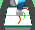
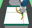
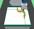
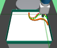
Let the starting and goal rope configurations be and . We find the cylinder position pair where , such that and are farthest from each other among all other cylinder pairs. Then, we perform a poke to drag towards . The position of the poke is kept close to , and poke direction is the direction from towards . After the poke execution, the next pair of farthest cylinder pair is again selected and another poke is executed. This is repeatedly done for pokes, until either the rope configuration comes within distance of goal , or we reach maximum episode horizon . Although, this policy is not the perfect policy for goal based rope manipulation, but it still is a good expert policy for collecting demonstrations . Moreover, as our method requires states and not primitive actions (pokes), we can use these demonstrations to collect good higher level subgoal dataset using primitive parsing.
A.3 Environment and implementation details
Here, we provide extensive environment and implementation details for various environments. We perform the experiments on two system each with Intel Core i7 processors, equipped with 48GB RAM and Nvidia GeForce GTX 1080 GPUs. We use expert demos for franks kitchen task and demos in all other tasks, and provide the procedures for collecting expert demos for all tasks in Appendix A.2. We empirically increased the number of demonstrations until there was no significant improvement in the performance. In our experiments, we use Soft Actor Critic [Haarnoja et al., 2018b]. The actor, critic and discriminator networks are formulated as layer fully connected networks with neurons in each layer.
When calculating , we normalize values of a trajectory before comparing with : for to . The experiments are run for , , , , , and timesteps in maze, pick and place, bin, hollow, rope and kitchen respectively. The regularization weight hyper-parameter is set at , , , , , and , the population hyper-parameter is set to be , , , , , and , and distance threshold hyper-parameter is set at , , , , , and for maze, pick and place, bin, hollow, rope and kitchen tasks respectively.
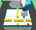
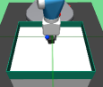
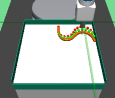
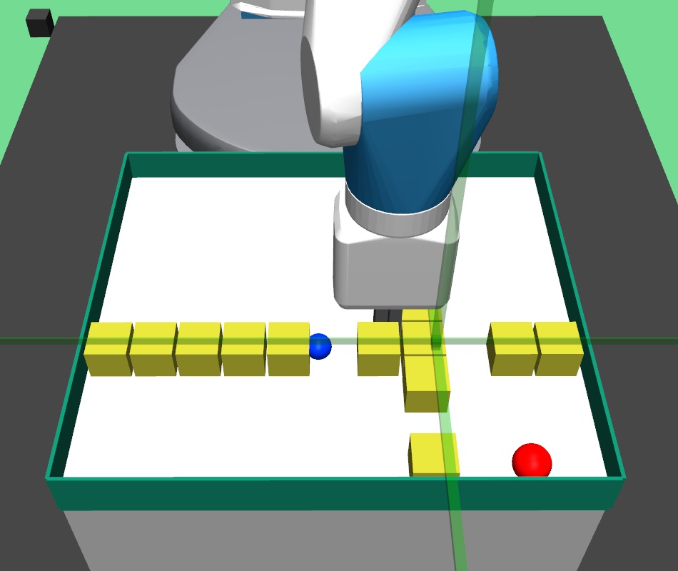
In maze navigation, a -DOF robotic arm navigates across randomly generated four room mazes, where the closed gripper (fixed at table height) has to navigate across the maze to the goal position. In pick and place task, the -DOF robotic arm gripper has to navigate to the square block, pick it up and bring it to the goal position. In bin task, the -DOF robotic arm gripper has to pick the square block and place the block inside the bin. In hollow task, the -DOF robotic arm gripper has to pick a square hollow block and place it such that a fixed vertical structure on the table goes through the hollow block. In rope manipulation task, a deformable soft rope is kept on the table and the -DoF robotic arm performs pokes to nudge the rope towards the desired goal rope configuration. The rope manipulation task involves learning challenging dynamics and goes beyond prior work on navigation-like tasks where the goal space is limited.
In the kitchen task, the -DoF franka robot has to perform a complex multi-stage task in order to achieve the final goal. Although many such permutations can be chosen, we formulate the following task: the robot has to first open the microwave door, then switch on the specific gas knob where the kettle is placed. In maze navigation, upper level predicts a subgoal, and the lower level primitive travels in a straight line towards the predicted goal. In pick and place, bin and hollow tasks, we design three primitives, gripper-reach: where the gripper goes to given position , gripper-open: opens the gripper, and gripper-close: closes the gripper. In kitchen environment, we use the action primitives implemented in RAPS [Dalal et al., 2021]. While using RAPS baseline, we hand designed action primitives, which we provide in detail in Section A.3.
A.3.1 Maze navigation task
In this environment, a -DOF robotic arm gripper navigates across random four room mazes. The gripper arm is kept closed and the positions of walls and gates are randomly generated. The table is discretized into a rectangular grid, and the vertical and horizontal wall positions and are randomly picked from and respectively. In the four room environment thus constructed, the four gate positions are randomly picked from , , and . The height of gripper is kept fixed at table height, and it has to navigate across the maze to the goal position(shown as red sphere).
The following implementation details refer to both the higher and lower level polices, unless otherwise explicitly stated. The state and action spaces in the environment are continuous. The state is represented as the vector , where is current gripper position and is the sparse maze array. The higher level policy input is thus a concatenated vector , where is the target goal position, whereas the lower level policy input is concatenated vector , where is the sub-goal provided by the higher level policy. The current position of the gripper is the current achieved goal. The sparse maze array is a discrete one-hot vector array, where represents presence of a wall block, and absence.
In our experiments, the size of and are kept to be and respectively. The upper level predicts subgoal , hence the higher level policy action space dimension is the same as the dimension of goal space of lower primitive. The lower primitive action which is directly executed on the environment, is a dimensional vector with every dimension . The first dimensions provide offsets to be scaled and added to gripper position for moving it to the intended position. The last dimension provides gripper control( implies a fully closed gripper, implies a half closed gripper and implies a fully open gripper). We select randomly generated mazes each for training, testing and validation. For selecting train, test and validation mazes, we first randomly generate distinct mazes, and then randomly divide them into train, test and validation mazes each. We use off-policy Soft Actor Critic [Haarnoja et al., 2018b] algorithm for optimizing RL objective in our experiments.
A.3.2 Pick and place, Bin and Hollow Environments
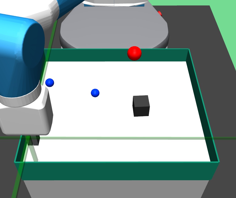
In the pick and place environment, a -DOF robotic arm gripper has to pick a square block and bring/place it to a goal position. We set the goal position slightly higher than table height. In this complex task, the gripper has to navigate to the block, close the gripper to hold the block, and then bring the block to the desired goal position. In the bin environment, the -DOF robotic arm gripper has to pick a square block and place it inside a fixed bin. In the hollow environment, the -DOF robotic arm gripper has to pick a hollow plate from the table and place it on the table such that its hollow center goes through a fixed vertical pole placed on the table.
In all the three environments, the state is represented as the vector , where is current gripper position, is the position of the block object placed on the table, is the relative position of the block with respect to the gripper, and consists of linear and angular velocities of the gripper and the block object. The higher level policy input is thus a concatenated vector , where is the target goal position. The lower level policy input is concatenated vector , where is the sub-goal provided by the higher level policy. The current position of the block object is the current achieved goal.
In our experiments, the sizes of , , , are kept to be , , and respectively. The upper level predicts subgoal , hence the higher level policy action space and goal space have the same dimension. The lower primitive action is a dimensional vector with every dimension . The first dimensions provide gripper position offsets, and the last dimension provides gripper control ( means closed gripper and means open gripper). While training, the position of block object and goal are randomly generated (block is always initialized on the table, and goal is always above the table at a fixed height). We select random each for training, testing and validation. For selecting train, test and validation mazes, we first randomly generate distinct environments with different block and target goal positions, and then randomly divide them into train, test and validation mazes each. We use off-policy Soft Actor Critic [Haarnoja et al., 2018b] algorithm for the RL objective in our experiments.
A.3.3 Rope Manipulation Environment
In the robotic rope manipulation task, a deformable rope is kept on the table and the robotic arm performs pokes to nudge the rope towards the desired goal rope configuration. The task horizon is fixed at pokes. The deformable rope is formed from constituent cylinders joined together. The following implementation details refer to both the higher and lower level polices, unless otherwise explicitly stated. The state and action spaces in the environment are continuous. The state space for the rope manipulation environment is a vector formed by concatenation of the intermediate joint positions. The upper level predicts subgoal for the lower primitive. The action space of the poke is , where is the initial position of the poke, and is the angle describing the direction of the poke. We fix the poke length to be .
While training our hierarchical approach, we select 100 randomly generated initial and final rope configurations each for training, testing and validation. For selecting train, test and validation configurations, we first randomly generate distinct configurations, and then randomly divide them into 100 train, test and validation mazes each. We use off-policy Soft Actor Critic [Haarnoja et al., 2018b] algorithm for optimizing RL objective in our experiments.
A.3.4 Impact Statement
Our proposed approach and algorithm are not anticipated to result in immediate technological advancements. Instead, our main contributions are conceptual, targeting fundamental aspects of Hierarchical Reinforcement Learning (HRL). By introducing primitive-enabled regularization, we present a novel framework that we believe holds significant potential to advance HRL research and its related fields. This conceptual groundwork lays the foundation for future investigations and could drive progress in HRL and associated domains.
A.4 Ablation experiments
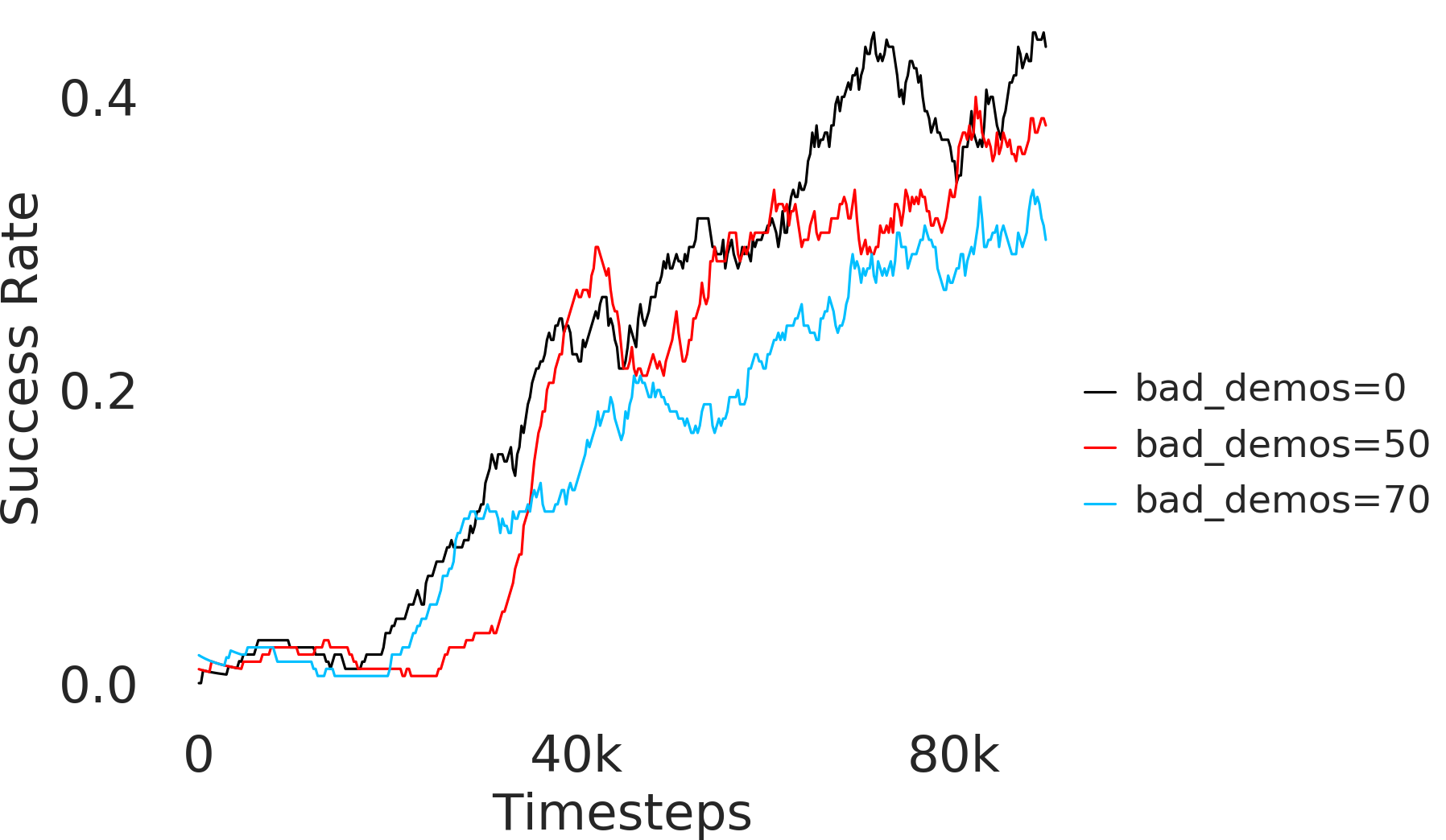
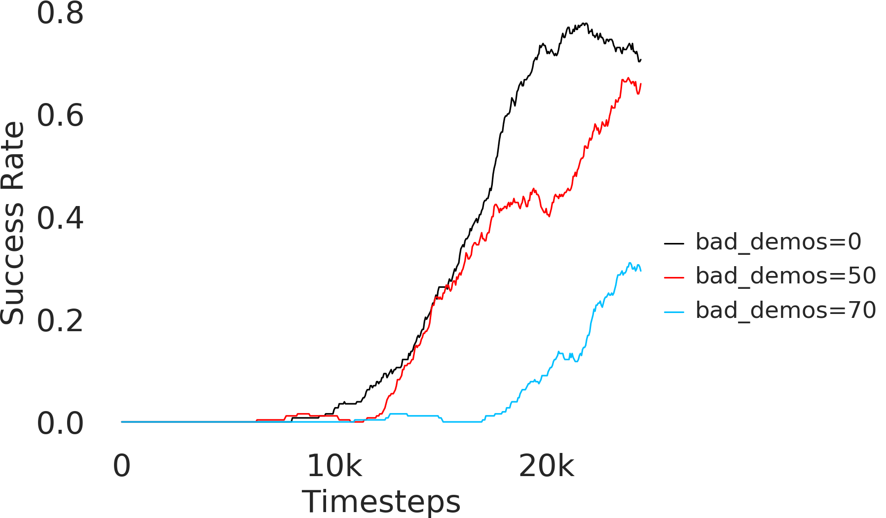
Here, we present the ablation experiments in all six task environments. The ablation analysis includes comparison with HAC-demos and HBC (Hierarchical behavior cloning) (Figure 14), choosing RPL hyperparameter (Figure 8), hyperparameter (Figure 9), RPL window size hyperparameter (Figure 10), learning weight hyperparameter (Figure 11), comparisons with varying number of expert demonstrations used during relabeling and training (Figure 12), comparison with HER-BC ablation (Figure 13), effect of sub-optimal demonstrations (Figure 15).


A.5 Qualitative visualizations
In this subsection, we provide visualizations for various environments.