Performance of Hybrid-ARQ in Block-Fading Channels: A Fixed Outage Probability Analysis
Abstract
This paper studies the performance of hybrid-ARQ (automatic repeat request) in Rayleigh block-fading channels. The long-term average transmitted rate is analyzed in a fast-fading scenario where the transmitter only has knowledge of channel statistics, and, consistent with contemporary wireless systems, rate adaptation is performed such that a target outage probability (after a maximum number of H-ARQ rounds) is maintained. H-ARQ allows for early termination once decoding is possible, and thus is a coarse, and implicit, mechanism for rate adaptation to the instantaneous channel quality. Although the rate with H-ARQ is not as large as the ergodic capacity, which is achievable with rate adaptation to the instantaneous channel conditions, even a few rounds of H-ARQ make the gap to ergodic capacity reasonably small for operating points of interest. Furthermore, the rate with H-ARQ provides a significant advantage compared to systems that do not use H-ARQ and only adapt rate based on the channel statistics.
I Introduction
ARQ (automatic repeat request) is an extremely powerful type of feedback-based communication that is extensively used at different layers of the network stack. The basic ARQ strategy adheres to the pattern of transmission followed by feedback of an ACK/NACK to indicate successful/unsuccessful decoding. If simple ARQ or hybrid-ARQ (H-ARQ) with Chase combining (CC) [1] is used, a NACK leads to retransmission of the same packet in the second ARQ round. If H-ARQ with incremental redundancy (IR) is used, the second transmission is not the same as the first and instead contains some “new” information regarding the message (e.g., additional parity bits). After the second round the receiver again attempts to decode, based upon the second ARQ round alone (simple ARQ) or upon both ARQ rounds (H-ARQ, either CC or IR). The transmitter moves on to the next message when the receiver correctly decodes and sends back an ACK, or a maximum number of ARQ rounds (per message) is reached.
ARQ provides an advantage by allowing for early termination once sufficient information has been received. As a result, it is most useful when there is considerably uncertainty in the amount/quality of information received. At the network layer, this might correspond to a setting where the network congestion is unknown to the transmitter. At the physical layer, which is the focus of this paper, this corresponds to a fading channel whose instantaneous quality is unknown to the transmitter.
Although H-ARQ is widely used in contemporary wireless systems such as HSPA [2], WiMax [3] (IEEE 802.16e) and 3GPP LTE [4], the majority of research on this topic has focused on code design, e.g., [5], [6], [7], while relatively little research has focused on performance analysis of H-ARQ [8]. Most relevant to the present work, in [9] Caire and Tuninetti established a relationship between H-ARQ throughput and mutual information in the limit of infinite block length. For multiple antenna systems, the diversity-multiplexing-delay tradeoff of H-ARQ was studied by El Gamal et al. [10], and the coding scheme achieving the optimal tradeoff was introduced; Chuang et al. [11] considered the optimal SNR exponent in the block-fading MIMO (multiple-input multiple-output) H-ARQ channel with discrete input signal constellation satisfying a short-term power constraint. H-ARQ has also been recently studied in quasi-static channels (i.e., the channel is fixed over all H-ARQ rounds) [12], [13] and shown to bring benefits to secrecy [14].
In this paper we build upon the results of [9] and perform a mutual information-based analysis of H-ARQ in block-fading channels. We consider a scenario where the fading is too fast to allow instantaneous channel quality feedback to the transmitter, and thus the transmitter only has knowledge of the channel statistics, but nonetheless each transmission experiences only a limited degree of channel selectivity. In this setting, rate adaptation can only be performed based on channel statistics and achieving a reasonable error/outage probability generally requires a conservative choice of rate if H-ARQ is not used. On the other hand, H-ARQ allows for implicit rate adaptation to the instantaneous channel quality because the receiver terminates transmission once the channel conditions experienced by a codeword are good enough to allow for decoding.
We analyze the long-term average transmitted rate achieved with H-ARQ, assuming that there is a maximum number of H-ARQ rounds and that a target outage probability at H-ARQ termination cannot be exceeded. We compare this rate to that achieved without H-ARQ in the same setting as well as to the ergodic capacity, which is the achievable rate in the idealized setting where instantaneous channel information is available to the transmitter. The main findings of the paper are that (a) H-ARQ generally provides a significant advantage over systems that do not use H-ARQ but have an equivalent level of channel selectivity, (b) the H-ARQ rate is reasonably close to the ergodic capacity in many practical settings, and (c) the rate with H-ARQ is much less sensitive to the desired outage probability than an equivalent system that does not use H-ARQ.
The present work differs from prior literature in a number of important aspects. One key distinction is that we consider systems in which the rate is adapted to the average SNR such that a constant target outage probability is maintained at all SNR’s, whereas most prior work has considered either fixed rate (and thus decreasing outage) [11] or increasing rate and decreasing outage as in the diversity-multiplexing tradeoff framework [10][15]. The fixed outage paradigm is consistent with contemporary wireless systems where an outage level near 1% is typical (see [16] for discussion), and certain conclusions depend heavily on the outage assumption. With respect to [9], note that the focus of [9] is on multi-user issues, e.g., whether or not a system becomes interference-limited at high SNR in the regime of very large delay, whereas we consider single-user systems and generally focus on performance with short delay constraints (i.e., maximum number of H-ARQ rounds). In addition, we use the attempted transmission rate, rather than the successful rate (which is used in [9]), as our performance metric. This is motivated by applications such as Voice-over-IP (VoIP), where a packet is dropped (and never retransmitted) if it cannot be decoded after the maximum number of H-ARQ rounds and quality of service is maintained by achieving the target (post-H-ARQ) outage probability. On the other hand, reliable data communication requires the use of higher-layer retransmissions whenever H-ARQ outages occur; in such a setting, the relevant metric is the successful rate, which is the product of the attempted transmission rate and the success probability (i.e., one minus the post-H-ARQ outage probability). If the post-H-ARQ outage is fixed to some target value (e.g., ), then studying the attempted rate is effectively equivalent to studying the successful rate.111If the post-H-ARQ outage probability can be optimized, then a careful balancing between the attempted rate and higher-layer retransmissions should be conducted in order to maximize the successful rate. Although this is beyond the scope of the present paper, note that some results in this direction can be found in [17] [18].
II System Model
We consider a block-fading channel where the channel remains constant over a block but varies independently from one block to another. The -th received symbol in the i-th block is given by:
| (1) |
where the index indicates the block number, indexes channel uses within a block, SNR is the average received SNR, is the fading channel coefficient in the -th block, and and are the transmitted symbol, received symbol, and additive noise, respectively. It is assumed that is complex Gaussian (circularly symmetric) with unit variance and zero mean, and that are i.i.d.. The noise has the same distribution as and is independent across channel uses and blocks. The transmitted symbol is constrained to have unit average power; we consider Gaussian inputs, and thus has the same distribution as the fading and the noise. Although we focus only on Rayleigh fading and single antenna systems, our basic insights can be extended to incorporate other fading distributions and MIMO as discussed in Section IV (Remark 1).
We consider the setting where the receiver has perfect channel state information (CSI), while the transmitter is aware of the channel distribution but does not know the instantaneous channel quality. This models a system in which the fading is too fast to allow for feedback of the instantaneous channel conditions from the receiver back to the transmitter, i.e., the channel coherence time is not much larger than the delay in the feedback loop. In cellular systems this is the case for moderate-to-high velocity users. This setting is often referred to as open-loop because of the lack of instantaneous channel tracking at the transmitter, although other forms of feedback, such as H-ARQ, are permitted. The relevant performance metrics, notably what we refer to as outage probability and fixed outage transmitted rate, are specified at the beginning of the relevant sections.
If H-ARQ is not used, we assume each codeword spans fading blocks; is therefore the channel selectivity experienced by each codeword. When H-ARQ is used, we make the following assumptions:
-
•
The channel is constant within each H-ARQ round ( symbols), but is independent across H-ARQ rounds.222An intuitive but somewhat misleading extension of the quasi-static fading model to the H-ARQ setting is to assume that the channel is constant for the duration of the H-ARQ rounds corresponding to a particular message/codeword, but is drawn independently across different messages. Because more H-ARQ rounds are needed to decode when the channel quality is poor, such a model actually changes the underlying fading distribution by increasing the probability of poor states and reducing the probability of good channel states. In this light, it is more accurate model the channel across H-ARQ rounds according to a stationary and ergodic random process with a high degree of correlation.
-
•
A maximum of H-ARQ rounds are allowed. An outage is declared if decoding is not possible after rounds, and this outage probability can be no larger than the constraint .
Because the channel is assumed to be independent across H-ARQ rounds, is the maximum amount of channel selectivity experienced by a codeword. When comparing H-ARQ and no H-ARQ, we set such that maximum selectivity is equalized.
It is worth noting that these assumptions on the channel variation are quite reasonable for the fast-fading/open-loop scenarios. Transmission slots in modern systems are typically around one millisecond, during which the channel is roughly constant even for fast fading. 333Frequency-domain channel variation within each H-ARQ round is briefly discussed in Section IV-B. An H-ARQ round generally corresponds to a single transmission slot, but subsequent ARQ rounds are separated in time by at least a few slots to allow for decoding and ACK/NACK feedback; thus the assumption of independent channels across H-ARQ rounds is reasonable. Moreover, a constraint on the number of H-ARQ rounds limits complexity (the decoder must retain information received in prior H-ARQ rounds in memory) and delay.
Throughout the paper we use the notation to denote the solution to the equation , where is a random variable; this quantity is well defined wherever it is used.
III Performance Without H-ARQ: Fixed-Length Coding
We begin by studying the baseline scenario where H-ARQ is not used and every codeword spans fading blocks. In this setting the outage probability is the probability that mutual information received over the fading blocks is smaller than the transmitted rate [19, eq (5.83)]:
| (2) |
where is the channel in the -th fading block. The outage probability reasonably approximates the decoding error probability for a system with strong coding [20] [21], and the achievability of this error probability has been rigorously shown in the limit of infinite block length () [22] [23].
Because the outage probability is a non-decreasing function of , by setting the outage probability to and solving for we get the following straightforward definition of -outage capacity [24]:
Definition 1
The -outage capacity with outage constraint and diversity order , denoted by , is the largest rate such that the outage probability in (2) is no larger than :
| (3) |
Using notation introduced earlier, the -outage capacity can be rewritten as
| (4) | |||||
| (5) |
For , can be written in closed form and inverted to yield [19]. For the outage probability cannot be written in closed form nor inverted, and therefore must be numerically computed. There are, however, two useful approximations to -outage capacity. The first one is the high-SNR affine approximation [25], which adds a constant rate offset term to the standard multiplexing gain characterization.
Theorem 1
The high-SNR affine approximation to -outage capacity is given by
| (6) |
where the notation implies that the term vanishes as .
Proof:
The proof is identical to that of the high-SNR offset characterization of MIMO channels in [26, Theorem 1], noting that single antenna block fading is equivalent to a MIMO channel with a diagonal channel matrix. ∎
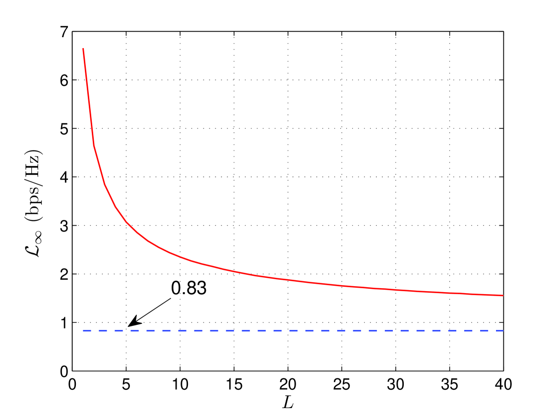
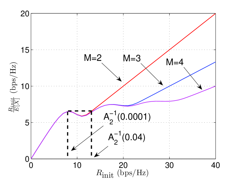
In terms of standard high SNR notation where [25][27], the multiplexing gain and the rate offset . The rate offset is the difference between the -outage capacity and the capacity of an AWGN channel with signal-to-noise ratio SNR. Although a closed form expression for cannot be found for , from [28],
| (7) |
where is the Meijer G-function [29, eq. (9.301)]. Based on (6), therefore is the solution to . The rate offset is plotted versus in Fig. 1 for . As the offset converges to , the offset of the ergodic Rayleigh channel [27].
While the affine approximation is accurate at high SNR’s, motivated by the Central Limit Theorem (CLT), an approximation that is more accurate for moderate and low SNR’s is reached by approximating random variable by a Gaussian random variable with the same mean and variance [30][31]. The mean and variance of are given by [32][33]:
| (8) | |||||
| (9) |
where , and at high SNR the standard deviation converges to [33]. The mutual information is thus approximated by a , and therefore
| (10) |
where is the tail probability of a unit variance normal. Setting this quantity to and then solving for yields an -outage capacity approximation [30, eq. (26)]:
| (11) |
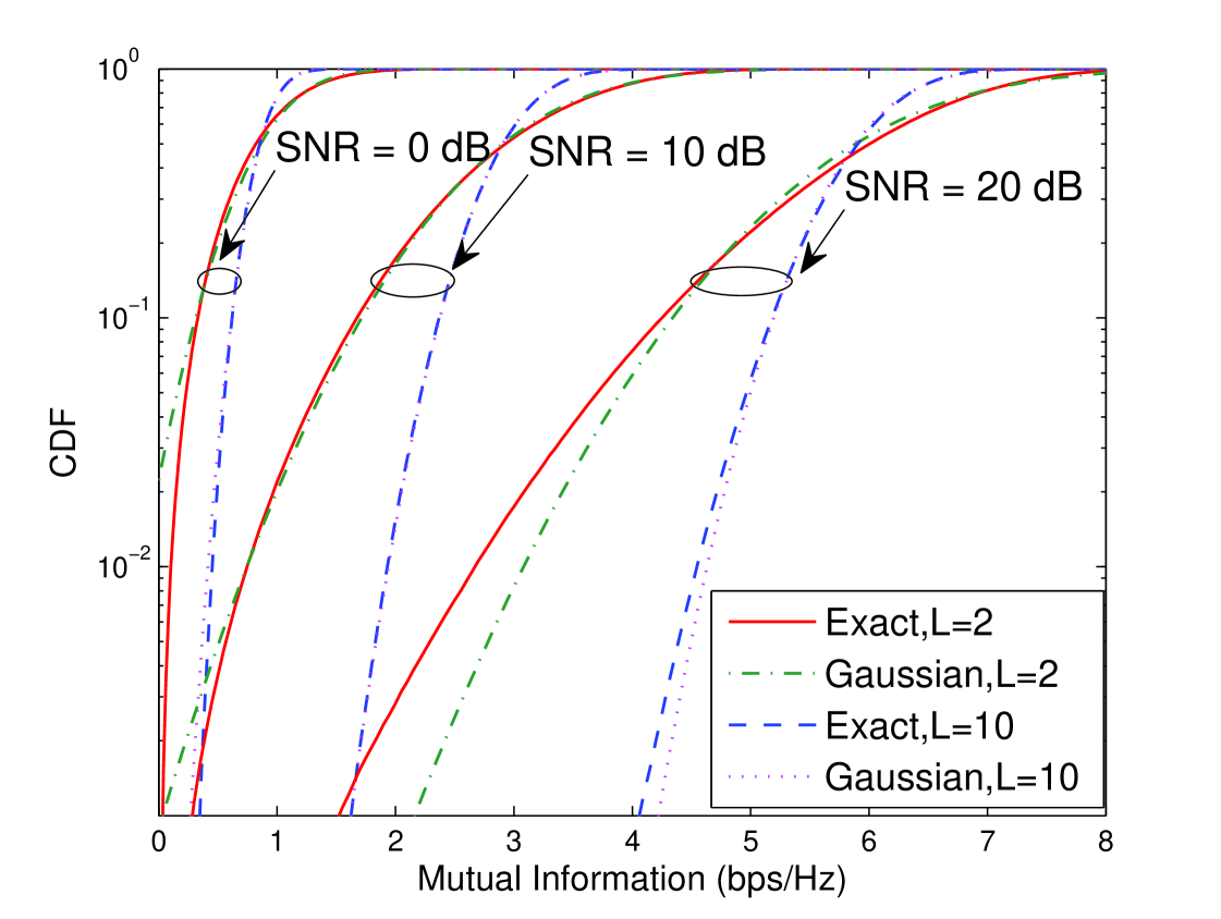
The accuracy of this approximation depends on how accurately the CDF of a Gaussian matches the CDF (i.e., outage probability) of random variable . In Fig. 2 both CDF’s are plotted for and , and , , and dB. As expected by the CLT, as increases the approximation becomes more accurate. Furthermore, the match is less accurate for very small values of because the tails of the Gaussian and the actual random variable do not precisely match. Finally, note that the match is not as accurate at low SNR’s: this is because the mutual information random variable has a density close to a chi-square in this regime, and is thus not well approximated by a Gaussian. Although not accurate in all regimes, numerical results confirm that the Gaussian approximation is reasonably accurate for the range of interest for parameters (e.g., and dB). More importantly, this approximation yields important insights.
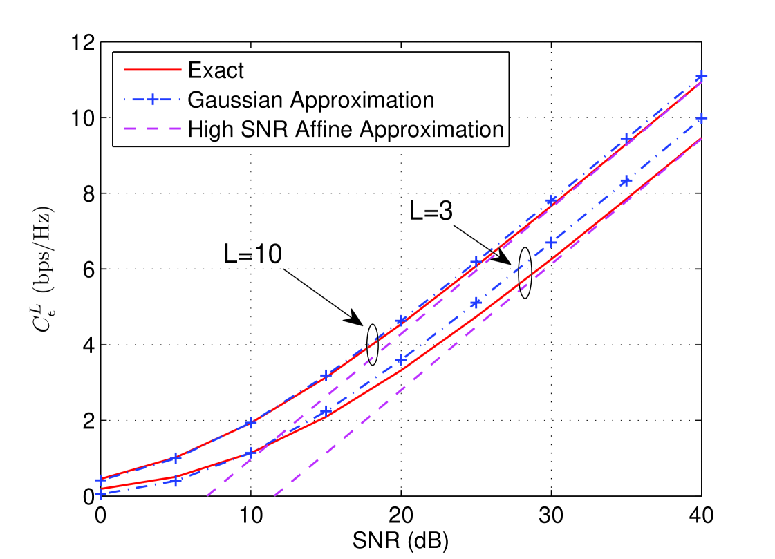
In Fig. 3 the true -outage capacity and the affine and Gaussian approximations are plotted versus SNR for and . The Gaussian approximation is reasonably accurate at moderate SNR’s, and is more accurate for larger values of . On the other hand, the affine approximation, which provides a correct high SNR offset, is asymptotically tight at high SNR.
III-A Ergodic Capacity Gap
When evaluating the effect of the diversity order , it is useful to compare the ergodic capacity and . By Chebyshev’s inequality, for any ,
| (12) |
By replacing with and equating the right hand side (RHS) with , we get
| (13) |
This implies as , as intuitively expected; reasonable values of are smaller than , and thus we expect convergence to occur from below.
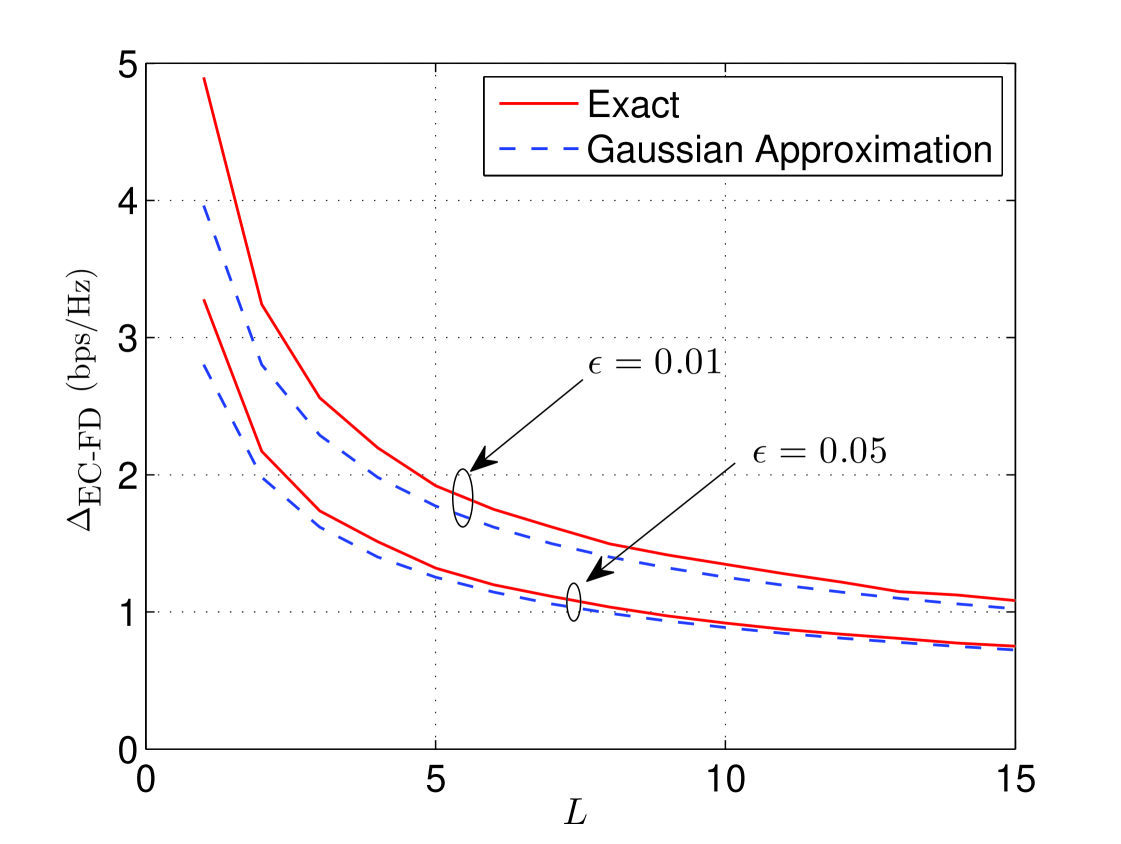
In order to capture the speed at which this convergence occurs, we define the quantity as the difference between the ergodic and -outage capacities. Based on (13) we can upper bound as:
| (14) |
This bound shows that the rate gap goes to zero at least as fast as . Although we cannot rigorously claim that is of order , by (11) the Gaussian approximation to this quantity is:
| (15) |
which is also . This approximation becomes more accurate as , by the CLT, and thus is expected to correctly capture the scaling with . Note that (15) has the interpretation that the rate must be deviations below the ergodic capacity in order to ensure reliability. In Fig. 4 the actual capacity gap and the approximation in (15) are plotted for and with dB, and a reasonable match between the approximation and the exact gap is seen.
IV Performance with Hybrid-ARQ
We now move on to the analysis of hybrid-ARQ, which will be shown to provide a significant performance advantage relative to the baseline of non-H-ARQ performance. H-ARQ is clearly a variable-length code, in which case the average transmission rate must be suitably defined. If each message contains information bits and each ARQ round corresponds to channel symbols, then the initial transmission rate is bits/symbol. If random variable denotes the number of H-ARQ rounds used for the -th message, then a total of H-ARQ rounds are used and the average transmission rate (in bits/symbol or bps/Hz) across those messages is:
| (16) |
We are interested in the long-term average transmission rate, i.e., the case where . By the law of large numbers (note that the ’s are i.i.d. in our model), and thus the rate converges to
| (17) |
Here is the random variable representing the number of H-ARQ rounds per message; this random variable is determined by the specifics of the H-ARQ protocol.
In the remainder of the paper we focus on incremental redundancy (IR) H-ARQ because it is the most powerful type of H-ARQ, although we compare IR to Chase combining in Section IV-E. In [9] it is shown that mutual information is accumulated over H-ARQ rounds when IR is used, and that decoding is possible once the accumulated mutual information is larger than the number of information bits in the message. Therefore, the number of H-ARQ rounds is the smallest number such that:
| (18) |
The number of rounds is upper bounded by , and an outage occurs whenever the mutual information after rounds is smaller than :
| (19) |
This is the same as the expression for outage probability of -order diversity without H-ARQ in (2), except that mutual information is summed rather than averaged over the rounds. This difference is a consequence of the fact that is defined for transmission over one round rather than all rounds; dividing by in (17) to obtain the average transmitted rate makes the expressions consistent. Due to this relationship, if the initial rate is set as , where is the -outage capacity for -order diversity without H-ARQ, then the outage at H-ARQ termination is .
In order to simplify expressions, it is useful to define as the probability that the accumulated mutual information after rounds is smaller than :
| (20) |
The expected number of H-ARQ rounds per message is therefore given by:
| (21) |
The long-term average transmitted rate, which is denoted as , is defined by (17). With initial rate we have:444All quantities in this expression except are actually functions of SNR. For the sake of compactness, however, dependence upon SNR is suppressed in this and subsequent expressions, except where explicit notation is necessary.
| (22) |
Note that is the attempted long-term average transmission rate, as discussed in Section I. For the sake of brevity this quantity is referred to as the H-ARQ rate; this is not to be confused with the initial rate . Similarly, we refer to -outage capacity as the non-H-ARQ rate in the rest of the paper.
Because , the H-ARQ rate is at least as large as the non-H-ARQ rate, i.e., , and the advantage with respect to the non-H-ARQ benchmark is precisely the multiplicative factor . This difference is explained as follows. Because , each message/packet contains information bits regardless of whether H-ARQ is used. Without H-ARQ these bits are always transmitted over symbols, whereas with H-ARQ an average of only symbols are required.
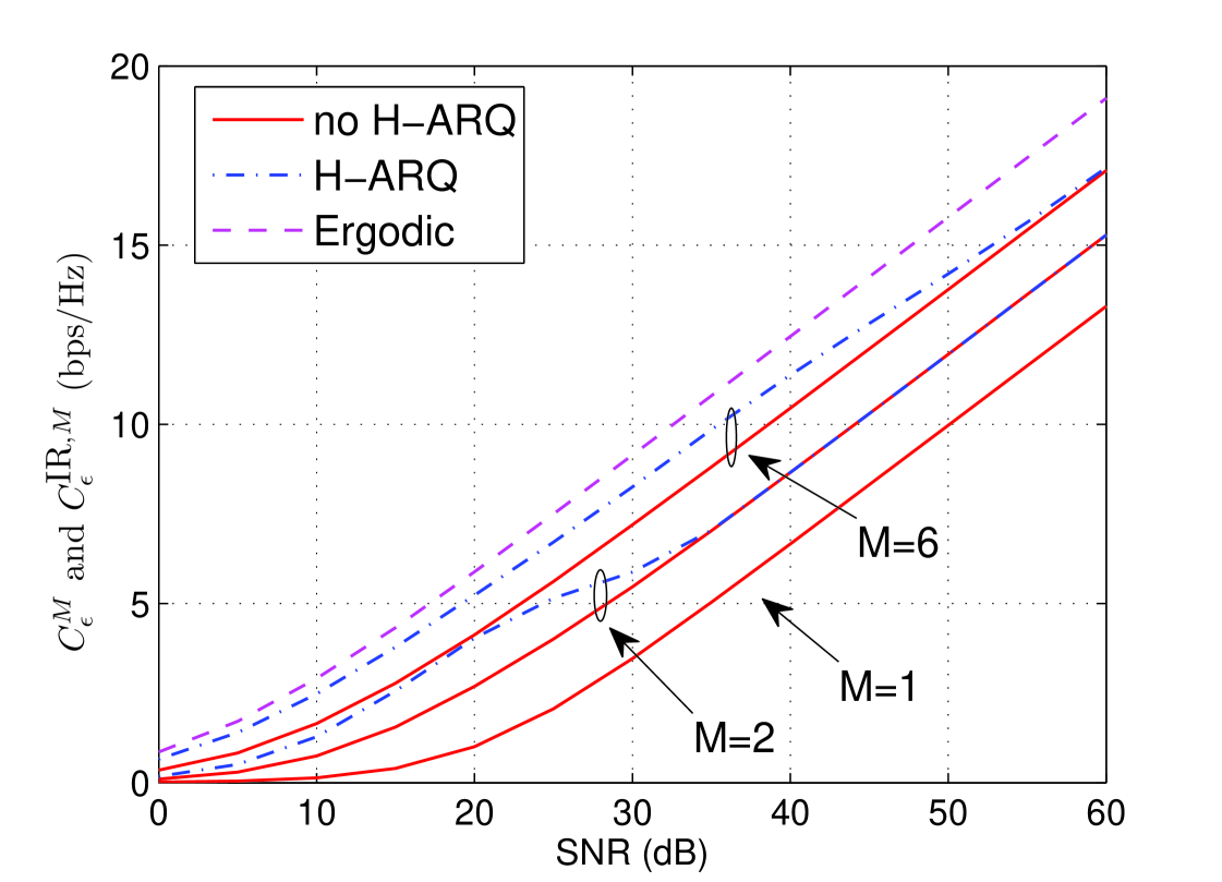
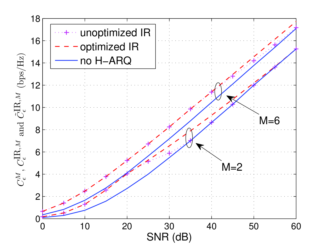
In Fig. 5 the average rates with () and without H-ARQ () are plotted versus SNR for and and ( does not allow for H-ARQ in our model). Ergodic capacity is also plotted as a reference. Based on the figure, we immediately notice:
-
•
H-ARQ with 6 rounds outperforms H-ARQ with 2 rounds.
-
•
H-ARQ provides a significant advantage relative to non-H-ARQ for the same value of for a wide range of SNR’s, but this advantage vanishes at high SNR.
Increasing rate with is to be expected, because larger corresponds to more time diversity and more early termination opportunities. The behavior with respect to SNR is perhaps less intuitive. The remainder of this section is devoted to quantifying and explaining the behavior seen in Fig. 5. We begin by extending the Gaussian approximation to H-ARQ, then examine performance scaling with respect to , SNR, and , and finally compare IR to Chase Combining.
IV-A Gaussian Approximation
By the definition of and (21)-(22), the H-ARQ rate can be written as:
| (23) |
where refers to the inverse of function . If we use the approach of Section III and approximate the mutual information accumulated in rounds by a Gaussian with mean and variance , where and are defined in (8) and (9), we have:
| (24) |
Similar to (11), the initial rate can be approximated as . Applying the approximation of to each term in (23) and using the property yields:
| (25) |
This approximation is easier to compute than the actual H-ARQ rate and is reasonably accurate. Furthermore, it is useful for the insights it can provide.
IV-B Scaling with H-ARQ Rounds
In this section we study the dependence of the H-ARQ rate on . We first show convergence to the ergodic capacity as :
Theorem 2
For any SNR, the H-ARQ rate converges to the ergodic capacity as :
| (26) |
Proof:
See Appendix A. ∎
To quantify how fast this convergence is, similar to Section III-A we investigate the difference between the ergodic capacity and the H-ARQ rate. Defining we have
| (27) |
where the approximation follows from in (11). Because is on the order of (as established in the proof of Theorem 2), the key is the behavior of the term .
To better understand we again return to the Gaussian approximation. While the CDF of is defined by (for ), we use to denote the random variable using the Gaussian approximation and thus define its CDF (for integers ) as:
| (28) |
where we have used evaluated with . From this expression, we can immediately see that the median of is [34]. If this was equal to the mean of , then by (27) the rate difference would be well approximated by , where is the difference between and and thus is no larger than one. By studying the characteristics of (and of ) we can see that the median is in fact quite close to the mean. A tedious calculation in Appendix B gives the following approximation to :
| (29) |
which is reasonably accurate for large . The most important factor is the term , which is due to the fact that only an integer number of H-ARQ rounds can be used. The factor exists because the random variable is truncated at the point where its CDF is .
Applying this into (27), the rate difference can be approximated as:
| (30) |
The denominator increases with at the order of (more precisely as ), while the numerator actually decreases with and can even become negative if is extremely large. For reasonable values of , however, the negative term in the numerator is essentially inconsequential (for example, if and dB, the negative term is much smaller than for ) and thus can be reasonably neglected. By ignoring this negative term and replacing the denominator with the leading order term, we get a further approximation of the rate gap:
| (31) |
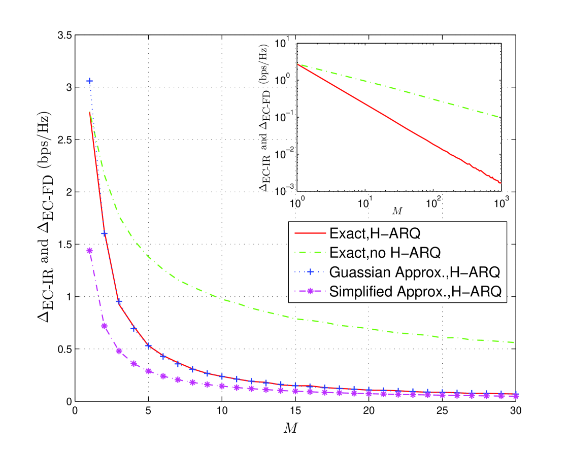
Based on this approximation, we see that the rate gap decreases roughly on the order , rather than the decrease without H-ARQ. In Fig. 6 we plot the exact capacity gap with and without H-ARQ, as well as the Gaussian approximation to the H-ARQ gap (30) and its simplified form in (31) for at dB. Both approximations are seen to be reasonably accurate especially for large . In the inset plot, which is in log-log scale, we see that the exact capacity gap goes to zero at order , consistent with the result obtained from our approximation.
The fast convergence with H-ARQ can be intuitively explained as follows. If transmission could be stopped precisely when enough mutual information has been received, the transmitted rate would be exactly matched to the instantaneous mutual information and thus ergodic capacity would be achieved. When H-ARQ is used, however, transmission can only be terminated at the end of a round as, opposed to within a round, and thus a small amount of the transmission can be wasted. This ”rounding error”, which is reflected in the term in (30) and (31), is essentially the only penalty incurred by using H-ARQ rather than explicit rate adaptation.
Remark 1
Because the value of H-ARQ depends primarily on the mean and variance of the mutual information in each H-ARQ round, our basic insights can be extended to multiple-antenna channels and to channels with frequency (or time) diversity within each ARQ round if the change in mean and variance is accounted for. For example, with order frequency diversity the mutual information in the -th H-ARQ round becomes , where is the channel in the -th round on the -th frequency channel. The mean mutual information is unaffected, while the variance is decreased by a factor of .
IV-C Scaling with SNR
In this section we quantify the behavior of H-ARQ as a function of the average SNR.555 Because constant outage corresponds to the full-multiplexing point, the results of [10] imply that cannot have a multiplexing gain/pre-log larger than one (in [10] it is shown that H-ARQ does not increase the full multiplexing point). However, the DMT-based results of [10] do not provide rate-offset characterization as in Theorems 3 and 4. Fig. 5 indicated that the benefit of H-ARQ vanishes at high SNR, and the following theorem makes this precise:
Theorem 3
If SNR is taken to infinity while keeping fixed, the expected number of H-ARQ rounds converges to and the H-ARQ rate converges to , the non-H-ARQ rate with the same selectivity:
| (32) | |||
| (33) |
Proof:
See Appendix C. ∎
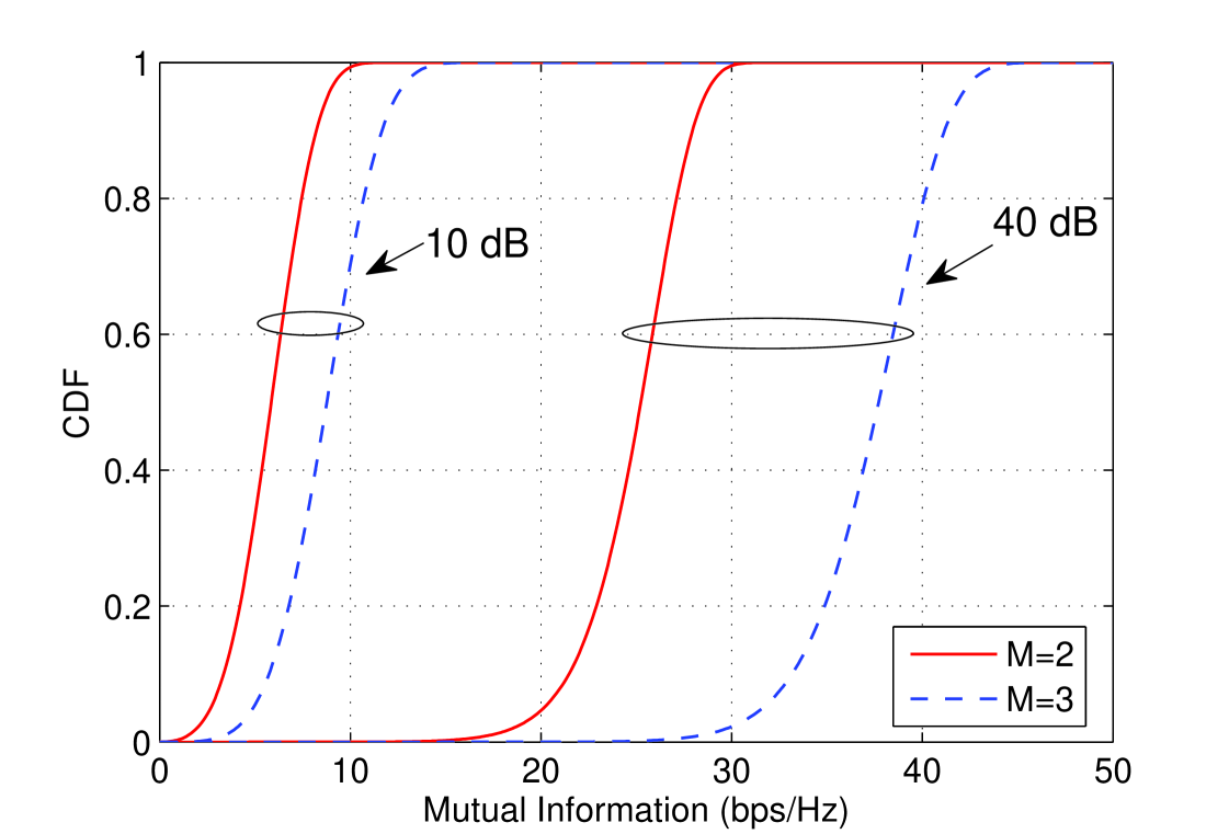
The intuition behind this result can be gathered from Fig. 7, where the CDF’s of the accumulated mutual information after and rounds are plotted for for and dB. If the initial rate is set at the -point of the CDF of . Because the CDF’s overlap for and considerably when dB, there is a large probability that sufficient mutual information is accumulated after rounds and thus early termination occurs. However, the overlap between these CDF’s disappears as SNR increases, because , and thus the early termination probability vanishes.
Although the H-ARQ advantage eventually vanishes, the advantage persists throughout a large SNR range and the Gaussian approximation (Section IV-A) can be used to quantify this. The probability of terminating in strictly less than rounds is approximated by:
| (34) |
In order for this approximation to be greater than one-half we require the numerator inside the -function to be less than zero, which corresponds to
| (35) |
As SNR increases increases without bound whereas converges to a constant. Thus increases quickly with SNR, which makes the probability of early termination vanish. From this we see that the H-ARQ advantage lasts longer (in terms of SNR) when is larger. The second inequality in (35) captures an alternative viewpoint, which is roughly the minimum value of required for H-ARQ to provide a significant advantage.
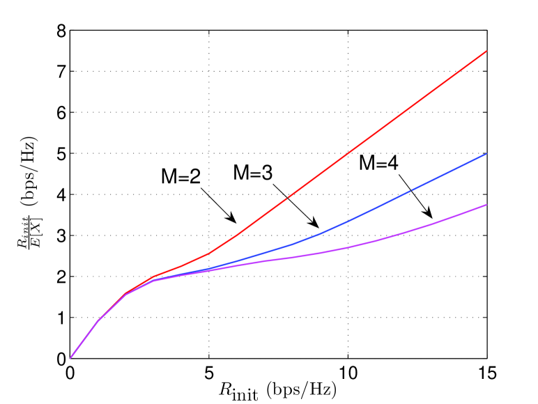
Motivated by naive intuition that the H-ARQ rate is monotonically increasing in the initial rate , up to this point we have chosen such that outage at H-ARQ termination is exactly . However, it turns out that the H-ARQ rate is not always monotonic in . In Fig. 8, the H-ARQ rate is plotted versus initial rate for and for dB (left) and dB (right). At dB, monotonically increases with and thus there is no advantage to optimizing the initial rate. At dB, however, behaves non-monotonically with . We therefore define as the maximized H-ARQ rate, where the maximization is performed over all values of initial rate such that the outage constraint is not violated:
| (36) |
The local maxima seen in Fig. 8 appear to preclude a closed form solution to this maximization. Although optimization of the initial rate provides an advantage over a certain SNR range, the following theorem shows that it does not provide an improvement in the high-SNR offset:
Theorem 4
H-ARQ with an optimized initial rate, i.e., , achieves the same high-SNR offset as unoptimized H-ARQ
| (37) |
Furthermore, the only initial rate (ignoring terms) that achieves the correct offset is the unoptimized value .
Proof:
See Appendix D. ∎
In Fig. 9, rates with and without optimization of the initial rate are plotted for and . For optimization begins to make a difference at the point where the unoptimized curve abruptly decreases towards around dB, but this advantage vanishes around dB. For the advantage of initial rate optimization comes about at a much higher SNR, consistent with (35). Convergence of to does eventually occur, but is not visible in the figure.
IV-D Scaling with Outage Constraint
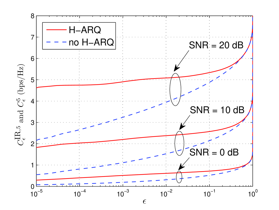
Another advantage of H-ARQ is that the H-ARQ rate is generally less sensitive to the desired outage probability than an equivalent non-H-ARQ system. This advantage is clearly seen in Fig. 10, where the H-ARQ and non-H-ARQ rates are plotted versus for at , and dB. When is large (e.g., roughly around ) H-ARQ provides almost no advantage: a large outage corresponds to a large initial rate, which in turn means early termination rarely occurs. However, for more reasonable values of , the H-ARQ rate is roughly constant with respect to whereas the non-H-ARQ rate decreases sharply as . The transmitted rate must be decreased in order to achieve a smaller (with or without H-ARQ), but with H-ARQ this decrease is partially compensated by the accompanying decreasing in the number of rounds .
IV-E Chase Combining
If Chase combining is used, a packet is retransmitted whenever a NACK is received and the receiver performs maximal-ratio-combining (MRC) on all received packets. As a result, SNR rather the mutual information is accumulated over H-ARQ rounds and the outage probability is given by:
| (38) |
For outage , the initial rate is .
Different from IR, the expected number of H-ARQ rounds in CC is not dependent on SNR and thus the average rate for outage can be written in closed form:
| (39) |
where the denominator is . According to (39), we can get the high SNR affine approximation as:
| (40) |
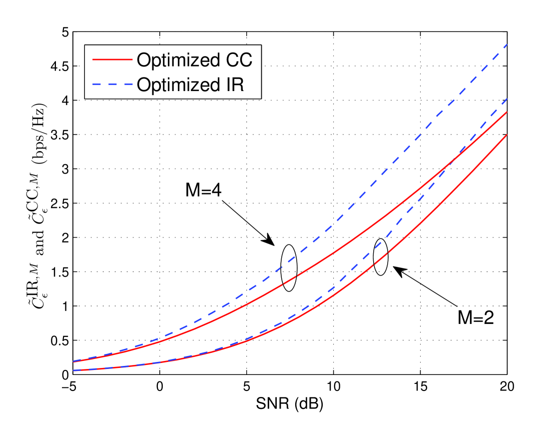
Because for any positive outage value, the pre-log factor (i.e., multiplexing gain) is and thus is less than one. This implies that CC performs poorly at high SNR. This is to be expected because CC is essentially a repetition code, which is spectrally inefficient at high SNR. As with IR, the performance of CC at high SNR can be improved through rate optimization. At high SNR, the pre-log is critical and thus the initial rate should be selected so that is close to one and thereby avoiding H-ARQ altogether. Even with optimization, CC is far inferior to IR at moderate and high SNR’s. On the other hand, CC performs reasonably well at low SNR. This is because for small values of , and thus SNR-accumulation is nearly equivalent to mutual information-accumulation. In Fig. 11 rate-optimized IR and CC are plotted for and , and the results are consistent with the above intuitions.
V Conclusion
In this paper we have studied the performance of hybrid-ARQ in the context of an open-loop/fast-fading system in which the transmission rate is adjusted as a function of the average SNR such that a target outage probability is not exceeded. The general findings are that H-ARQ provides a significant rate advantage relative to a system not using H-ARQ at reasonable SNR levels, and that H-ARQ provides a rate quite close to the ergodic capacity even when the channel selectivity is limited.
There appear to be some potentially interesting extensions of this work. Contemporary cellular systems utilize simple ARQ on top of H-ARQ, and it is not fully understood how to balance these reliability mechanisms; some results in this direction are presented in [17]. Although we have assumed error-free ACK/NACK feedback, such errors can be quite important (c.f., [35]) and merit further consideration. Finally, while we have considered only the mutual information of Gaussian inputs, it is of interest to extend the results to discrete constellations and possibly compare to the performance of actual codes.
VI Acknowledgments
The authors gratefully acknowledge Prof. Robert Heath for suggesting use of the Gaussian approximation, and Prof. Gerhard Wunder for suggesting use of Chebyshev’s inequality in Section III-A.
Appendix A PROOF OF THEOREM
Because and (Section III-A), we can prove by showing . Because , we can show this simply by showing is of order . For notational convenience we define , and then have:
| (41) | |||||
| (42) | |||||
| (43) |
where the first line holds because is increasing in and from (13), the second holds because the summands are non-negative, and the last line because the summands are decreasing in . A direct application of the CLT shows as , and thus, with some straightforward algebra, we have .
Appendix B PROOF OF (29)
Firstly, we relax the constraint on (discreteness and finiteness) to define a new continuous random variable , which is distributed along the whole real line. The CDF of (for all real ) is
| (44) |
Now if we consider the distribution of , we have
| (45) |
where the equality follows from (44). Notice as , , so
| (46) |
where is the standard normal CDF with zero mean and unit variance. So as , the limiting distribution of , denoted by , goes to , which is
| (47) |
Since is an approximation to , then we focus on evaluating for large :
| (48) | |||||
where (a) holds since when and (b) follows from and is negligible when is large enough. Actually, the first integral in (48) can be evaluated as because the expression inside the integral is symmetric with respect to and for any . For large , the second integral in (48) can be approximated as:
| (49) | |||||
where (a) follows from [36]: when is positive and large enough, . The last line holds because when M is sufficiently large [37]. This finally yields:
| (50) |
Appendix C PROOF OF THEOREM
In order to prove the theorem, we first establish the following lemma:
Lemma 1
If the initial rate has a pre-log of , i.e., , then
| for and | (51a) | ||||
| for and | (51b) |
Proof:
For notational convenience we use to denote the quantity . We prove the first result by using the fact that which yields:
| (52) | |||||
where the first equality follows because the ’s are i.i.d. exponential with mean SNR. The exponent behaves as . If this exponent goes to infinity. Because the term vanishes, is raised to a power converging to , and thus (52) converges to . This yields the result in (51b). To prove (51b) we combine the property with the same argument as above:
If , is raised to a power that converges to and thus we get (51b). ∎
We now move on to the proof of the theorem. Using the expression for in (21) we have:
| (53) |
Because has a pre-log of , the lemma implies that each of the terms converge to one and thus .
In terms of the high-SNR offset we have:
| (54) | |||||
where (a) holds because and , and (b) holds because and therefore the term does not effect the limit.
Because the additive terms defining in (21) are decreasing, we lower bound as
| (55) |
where the last inequality follows from (52). Plugging this bound into (54) yields:
where the last line follows from the binomial expansion. Because has a pre-log of , each of the terms is of the form for some and some constant , and thus the RHS of the last line is zero. Because , this shows .
Appendix D PROOF OF THEOREM
In order to prove that rate optimization does not increase the high-SNR offset, we need to consider all possible choices of the initial rate . We begin by considering all choices of with a pre-log of , i.e., satisfying . Because the proof of convergence of in the proof of Theorem only requires to have a pre-log of , we have . To bound the offset, we write the rate as where is strictly positive and sub-logarithmic (because the pre-log is ), and thus the rate offset is:
| (56) |
By the same argument as in Appendix C, the first term is upper bounded by zero in the limit. Therefore:
| (57) |
Relative to , the offset is either strictly negative (if is bounded) or goes to negative infinity. In either case a strictly worse offset is achieved.
Let us now consider pre-log factors, denoted by , strictly smaller than (i.e., ). We first consider non-integer values of . By Lemma 1 the first terms in the expression for converge to one while the other terms go to zero. Therefore . The long-term transmitted rate, given by , therefore has pre-log equal to . This quantity is strictly smaller than one, and therefore a non-integer yields average rate with a strictly suboptimal pre-log factor.
We finally consider integer values of satisfying . In this case we must separately consider rates of the form versus those of the form . Here we use to denote terms that are sub-logarithmic and that go to positive infinity; note that we also explicitly denote the sign of the or terms. We first consider . By Lemma 1 the terms corresponding to in the expression for converge to one, while the terms corresponding to go to one. Furthermore, the term corresponding to converges to a strictly positive constant denoted :
| (58) | |||||
where the second equality follows from [26]. is strictly positive because the support of , and thus of the sum, is the entire real line. As a result, , which is strictly larger than . The pre-log of the average rate is then , and so this choice of initial rate is also sub-optimal.
If the terms in the expression behave largely the same as above except that the term converges to one because the term in (58) is replaced with a quantity tending to positive infinity. Therefore , which also yields a sub-optimal pre-log of .
We are thus finally left with the choice . This is the same as the above case except that the term converges to zero. Therefore , and thus the achieved pre-log is one. In this case we must explicitly consider the rate offset, which is written as:
| (59) |
Using essentially the same proof as for Theorem , the difference between the first two terms is upper bounded by zero in the limit of . Thus, the rate offset goes to negative infinity.
Because we have shown each choice of (except ) achieves either a strictly sub-optimal pre-log or the correct pre-log but a strictly negative offset, this proves both parts of the theorem.
References
- [1] D. Chase, “Class of algorithms for decoding block codes with channel measurement information,” IEEE Trans. Inf. Theory, vol. 18, no. 1, pp. 170–182, 1972.
- [2] M. Sauter, Communications Systems for the Mobile Information Society. John Wiley, 2006.
- [3] J. G. Andrews, A. Ghosh, and R. Muhamed, Fundamentals of Wimax: Understanding Broadband Wireless Networking, 1st ed. Prentice Hall PTR, 2007.
- [4] L. Favalli, M. Lanati, and P. Savazzi, Wireless Communications 2007 CNIT Thyrrenian Symposium, 1st ed. Springer, 2007.
- [5] S. Sesia, G. Caire, and G. Vivier, “Incremental redundancy hybrid ARQ schemes based on low-density parity-check codes,” IEEE Trans. Commun., vol. 52, no. 8, pp. 1311–1321, Aug. 2004.
- [6] D. Costello, J. Hagenauer, H. Imai, and S. Wicker, “Applications of error-control coding,” IEEE Trans. Inf. Theory, vol. 44, no. 6, pp. 2531–2560, Oct. 1998.
- [7] E. Soljanin, N. Varnica, and P. Whiting, “Incremental redundancy hybrid ARQ with LDPC and raptor codes,” submitted to IEEE Trans. Inf. Theory, 2005.
- [8] C. Lott, O. Milenkovic, and E. Soljanin, “Hybrid ARQ: theory, state of the art and future directions,” IEEE Inf. Theory Workshop, pp. 1–5, Jul. 2007.
- [9] G. Caire and D. Tuninetti, “The throughput of hybrid-ARQ protocols for the Gaussian collision channel,” IEEE Trans. Inf. Theory, vol. 47, no. 4, pp. 1971–1988, Jul. 2001.
- [10] H. E. Gamal, G. Caire, and M. E. Damen, “The MIMO ARQ channel: diversity-multiplexing-delay tradeoff,” IEEE Trans. Inf. Theory, pp. 3601–3621, 2006.
- [11] A. Chuang, A. Guillén i Fàbregas, L. K. Rasmussen, and I. B. Collings, “Optimal throughput-diversity-delay tradeoff in MIMO ARQ block-fading channels,” IEEE Trans. Inf. Theory, vol. 54, no. 9, pp. 3968–3986, Sep. 2008.
- [12] C. Shen, T. Liu, and M. P. Fitz, “Aggressive transmission with ARQ in quasi-static fading channels,” Proc. of IEEE Int’l Conf. in Commun. (ICC’08), pp. 1092–1097, May 2008.
- [13] R. Narasimhan, “Throughput-delay performance of half-duplex hybrid-ARQ relay channels,” Proc. of IEEE Int’l Conf. in Commun. (ICC’08), pp. 986–990, May 2008.
- [14] X. Tang, R. Liu, P. Spasojevic, and H. V. Poor, “On the Throughput of Secure Hybrid-ARQ Protocols for Gaussian Block-Fading Channels,” IEEE Trans. Inf. Theory, vol. 55, no. 4, pp. 1575–1591, Apr. 2009.
- [15] L. Zheng and D. Tse, “Diversity and multiplexing: a fundamental tradeoff in multiple-antenna channels,” IEEE Trans. Inf. Theory, vol. 49, no. 5, pp. 1073–1096, May 2003.
- [16] A. Lozano and N. Jindal, “Transmit diversity v. spatial multiplexing in modern MIMO systems,” submitted to IEEE Trans. Wireless Commun., 2008.
- [17] P. Wu and N. Jindal, “Coding Versus ARQ in Fading Channels: How reliable should the PHY be?” submitted to Proc. of IEEE Globe Commum. Conf. (Globecom’09), 2009.
- [18] T. A. Courtade and R. D. Wesel, “A cross-layer perspective on rateless coding for wirelss channels,” to appear at Proc. of IEEE Int’l Conf. in Commun. (ICC’09), Jun. 2009.
- [19] D. Tse and P. Viswanath, Fundamentals of Wireless Communications. Cambridge University, 2005.
- [20] G. Carie, G. Taricco, and E. Biglieri, “Optimum power control over fading channels,” IEEE Trans. Inf. Theory, vol. 45, no. 5, pp. 1468–1489, Jul. 1999.
- [21] A. Guillén i Fàbregas and G. Caire, “Coded modulation in the block-fading channel: coding theorems and code construction,” IEEE Trans. Inf. Theory, vol. 52, no. 1, pp. 91–114, Jan. 2006.
- [22] N. Prasad and M. K. Varanasi, “Outage theorems for MIMO block-fading channels,” IEEE Trans. Inf. Theory, vol. 52, no. 12, pp. 5284–5296, Dec. 2006.
- [23] E. Malkamäki and H. Leib, “Coded diversity on block-fading channels,” IEEE Trans. Inf. Theory, vol. 45, no. 2, pp. 771–781, Mar. 1999.
- [24] S. Verdú and T. S. Han, “A general formula for channel capacity,” IEEE Trans. Inf. Theory, vol. 40, no. 4, pp. 1147–1157, Jul. 1994.
- [25] S. Shamai and S. Verdú, “The impact of frequency-flat fading on the spectral efficiency of CDMA,” IEEE Trans. Inf. Theory, vol. 47, no. 5, pp. 1302–1327, May 2001.
- [26] N. Prasad and M. Varanasi, “MIMO outage capacity in the high SNR regime,” Proc. of IEEE Int’l Symp. on Inform. Theory (ISIT’05), pp. 656–660, Sep. 2005.
- [27] A. Lozano, A. M. Tulino, and S. Verdú, “High-SNR power offset in multiantenna communication,” IEEE Trans. Inf. Theory, vol. 51, no. 12, pp. 4134–4151, Dec. 2005.
- [28] J. Salo, H. E. Sallabi, and P. Vainikainen, “The distribution of the product of independent Rayleigh random variables,” IEEE Trans. Antennas Propag., vol. 54, no. 2, pp. 639–643, Feb. 2006.
- [29] I. S. Gradshteyn and I. M. Ryzhik, Table of Integrals, Series, and Products, 5th ed. Academic, 1994.
- [30] G. Barriac and U. Madhow, “Characterizing outage rates for space-time communication over wideband channels,” IEEE Trans. Commun., vol. 52, no. 4, pp. 2198–2207, Dec. 2004.
- [31] P. J. Smith and M. Shafi, “On a Gaussian approximation to the capacity of wireless MIMO systems,” Proc. of IEEE Int’l Conf. in Commun. (ICC’02), pp. 406–410, Apr. 2002.
- [32] M. S. Alouini and A. J. Goldsmith, “Capacity of Rayleigh fading channels under different adaptive transmission and diversity-combining techniques,” IEEE Trans. Veh. Technol., vol. 48, no. 4, pp. 1165–1181, Jul. 1999.
- [33] M. R. McKay, P. J. Smith, H. A. Suraweera, and I. B. Collings, “On the mutual information distribution of OFDM-based spatial multiplexing: exact variance and outage approximation,” IEEE Trans. Inf. Theory, vol. 54, no. 7, pp. 3260–3278, 2008.
- [34] B. Fristedt and L. Gray, A Modern Approach to Probability Theory. Birkhäuser Boston, 1997.
- [35] M. Meyer, H. Wiemann, M. Sagfors, J. Torsner, and J.-F. Cheng, “ARQ concept for the UMTS long-term evolution,” Proc. of IEEE Vehic. Technol. Conf. (VTC’2006 Fall), Sep. 2006.
- [36] N. Kingsbury, “Approximation formula for the Gaussian error integral, Q(x),” http://cnx.org/content/m11067/latest/.
- [37] M. Abramowitz and I. A. Stegun, Handbook of Mathematical Functions with Formulas, Graphs, and Mathematical Tables. Dover Publications, 1964.