Perturbative and nonperturbative quasinormal modes of 4D Einstein-Gauss-Bonnet black holes
Abstract
We study the propagation of probe scalar fields in the background of 4D Einstein-Gauss-Bonnet black holes with anti-de Sitter (AdS) asymptotics and calculate the quasinormal modes. Mainly, we show that the quasinormal spectrum consists of two different branches, a branch perturbative in the Gauss–Bonnet coupling constant and another branch nonperturbative in . The perturbative branch consists of complex quasinormal frequencies that approximate to the quasinormal frequencies of the Schwarzschild AdS black hole in the limit of a null coupling constant. On the other hand, the nonperturbative branch consists of purely imaginary frequencies and is characterized by the growth of the imaginary part when decreases, diverging in the limit of null coupling constant, therefore they do not exist for the Schwarzschild AdS black hole. Also, we find that the imaginary part of the quasinormal frequencies is always negative for both branches; therefore, the propagation of scalar fields is stable in this background.
pacs:
04.40.-b, 95.30.Sf, 98.62.SbI Introduction
The Einstein-Gauss-Bonnet (EGB) gravity has been recently reformulated as the limit of their higher dimensional version when the coupling constant is rescaling as Glavan:2019inb . Thus,
the Gauss-Bonnet term shows a nontrivial contribution to the gravitational dynamics. The theory preserves the number of degrees of freedom and remains free from the Ostrogradsky instability. Also, the new theory
has stimulated a series of recent research works concerning to
black holes solutions and the properties of the novel 4D EGB theory, for instance, spherically symmetric black hole solutions were discovered Glavan:2019inb , generalizing the Schwarzschild black holes and are also free from singularity. Additionally, charged black holes in AdS spacetime Fernandes:2020rpa , radiating black holes solutions Ghosh:2020syx and an exact charged black hole surrounded by clouds of string was investigated Singh:2020nwo . The generalization of these static black holes to the rotating case was also addressed Wei:2020ght . On the other hand, regular black holes and the generalization of the BTZ solution in the presence of higher curvature (Gauss-Bonnet and Lovelock) corrections of any order was found in Refs. Kumar:2020uyz and Konoplya:2020ibi , respectively. Also, a Einstein-Lovelock theory was formulated and black hole solutions were studied in Konoplya:2020qqh ; Konoplya:2020der . The interesting physical properties of the black holes in this novel 4D Einstein-Gauss-Bonnet gravity has been investigated such as their thermodynamics Hegde:2020xlv ; HosseiniMansoori:2020yfj ; Wei:2020poh ; Singh:2020xju ; EslamPanah:2020hoj , Hawking radiation and greybody factors Zhang:2020qam ; Konoplya:2020cbv , quasinormal modes and stability Konoplya:2020bxa ; Konoplya:2020juj ; Mishra:2020gce ; Churilova:2020aca ; Zhang:2020sjh , geodesics motion and shadow Guo:2020zmf ; Heydari-Fard:2020sib ; Roy:2020dyy , electromagnetic radiation from a thin accretion disk from spherically symmetric black holes Liu:2020vkh , among others. However, recent works has raised criticisms about the approach applied in Ref. Glavan:2019inb , that arises from the idea of defining a theory from a set of solutions that are obtained by the limit of the -dimensional EGB theory, and there is an active debate on its validity, see for instance Gurses:2020ofy ; Mahapatra:2020rds ; Shu:2020cjw ; Tian:2020nzb . However, in Refs. Lu:2020iav ; Fernandes:2020nbq ; Hennigar:2020lsl have been proposed other approaches to obtain a well defined limit of EGB theory, and an action with a set of field equations were found, by using dimensional reduction methods Mann:1992ar ; Kobayashi:2020wqy .
The resulting theory corresponds to a scalar-tensor theory of the Horndeski type. It was shown that all the solutions found in the original paper on EGB theory Glavan:2019inb are also solutions of the new formulation of the theory. In particular, the spherically symmetric Schwarzschild-like solution generated by this theory coincides with the metric of the limit of the -dimensional EGB theory.
In the context of the detection of gravitational waves Abbott:2016blz , the quasinormal modes (QNMs) and quasinormal frequencies (QNFs) are important Regge:1957td ; Zerilli:1971wd ; Kokkotas:1999bd ; Nollert:1999ji ; Konoplya:2011qq . Despite the detected signal is consistent with the Einstein gravity TheLIGOScientific:2016src , there are possibilities for alternative theories of gravity due to the large uncertainties in mass and angular momenta of the ringing black hole Konoplya:2016pmh . It have been shown that the spectrum of QNMs of theories with higher curvature corrections, such as the Einstein-Gauss Bonnet gravity consists of two different branches Konoplya:2017ymp ; Gonzalez:2017gwa ; Grozdanov:2016fkt ; Grozdanov:2016vgg ; Gonzalez:2018xrq . One of them has an Einsteinian limit when the Gauss-Bonnet coupling constant tends to zero, while the other consists from purely imaginary modes of which the damping rate is increasing when decreases, these modes are qualitatively different from their Einsteinian analogues and they do not exists in the limit . This branch is, thereby, nonperturbative in Gonzalez:2017gwa 111Calling nonperturbative to this branch could sound inappropriate because it is derived by solving the linearized (perturbative) scalar equation..
The phenomena of nonperturbative modes seems to be general and independent on the asymptotic behavior of a black hole, topology of the event horizon, spin of the fields under consideration, and, possibly, even of the particular form of the higher curvature corrections to the General Relativity (GR). Thus, nowadays the study of nonperturbative modes has been a subject of interest, due to they may lead to a profile qualitatively different to the gravitational ringdown. On the other hand, from the gauge/gravity duality point of view, these modes lead to the eikonal instability of Gauss-Bonnet black holes at some critical values of coupling constant,
so that they determine possible constrains on holographic applicability of the black holes backgrounds. Moreover, it is worth to mentioning that the new nonperturbative modes were found for several quite different situation such as
the fourth order in curvature theory Grozdanov:2016fkt , asymptotically flat black holes Gleiser:2005ra ; Dotti:2005sq ; Takahashi:2010ye
and black branes.
In this work we consider 4D Einstein-Gauss-Bonnet black holes with anti-de Sitter (AdS) asymptotics and we study the propagation of scalar fields in such backgrounds, in order to show the existence of nonperturbative QNMs for this kind of theories. We obtain the QNFs numerically by using the pseudospectral Chebyshev method Boyd
which is an effective method to find high overtone modes, and that has been applied for instance in Refs. Finazzo:2016psx ; Gonzalez:2017shu . In spite of the criticisms on the original EGB, it is important to emphasize that the spherically symmetric Schwarzschild-like solution obtained in the limit of the -dimensional EGB theory, is also a solution of theories formulated with a well defined limit of EGB theory. Furthermore, it is worth to noting that these black holes are also solutions of the semi classical Einstein equation with Weyl anomaly Cai:2009ua and for a toy model of Einstein gravity with a Gauss-Bonnet classically “entropic” term mimicking a quantum correction Cognola:2013fva . Therefore, it is worthwhile to perform a study of the physical properties of these black holes, such as the propagation of matter field outside the event horizon.
The QNFs of scalar, electromagnetic and gravitational perturbations for this background in asymptotically flat spacetime were obtained recently in Ref. Konoplya:2020bxa , and it was shown that when the coupling constant is positive, the black hole is gravitationally unstable unless the coupling constant is small enough (). The instability develops at high multipole number , and therefore is known as eikonal instability. Also, the negative coupling constant allows for a stable black-hole solution up to relatively large absolute values of (). The QNFs of Dirac’s field, was studied in Ref. Churilova:2020aca , and it was shown that the real part of the QNFs is considerably increased, while the damping rate is usually decreasing when the coupling constant increased. Here, besides the perturbative modes, we will find nonperturbative modes in . When the metric corresponds to the Schwarzschild AdS black hole and the QNMs for this geometry were calculated in Ref. Horowitz:1999jd , where the approach to thermal equilibrium was established, and previously in Ref. Chan:1996yk .
II Einstein Gauss-Bonnet Black hole in four dimensional AdS spacetime
The Lagrangian of the -dimensional Einstein-Maxwell-Gauss-Bonnet theory with the coupling constant re-scaled by , is given by the relation Fernandes:2020rpa
| (1) |
where is the cosmological constant , is the Gauss-Bonnet term and is the electromagnetic field tensor. The solutions for a static and spherically symmetric ansatz in an arbitrary number of dimensions , has the form
| (2) |
where corresponds to -dimensional hypersurface. Then, following the prescription given in Glavan:2019inb and taking the limit it is possible to obtain the exact solution representing the 4D Einstein-Maxwell Gauss-Bonnet black hole Fernandes:2020rpa :
| (3) |
where is the mass of black hole and is its electric charge. From now on we will consider the uncharged version of the black hole metric:
| (4) |
Of the two branches of solution we are interested in the negative branch because it is the most physically interesting one; by taking appropriate limits it is possible to recover some special cases, for instance, when , Schwarzschild AdS (SAdS) black hole, and AdS spacetime () when and for null cosmological constant the seminal result found in Glavan:2019inb with the coupling parameter . It is worth to mention that similar metrics were found previously in the context of quantum corrections to gravity Tomozawa:2011gp ; Cai:2009ua ; Cognola:2013fva .
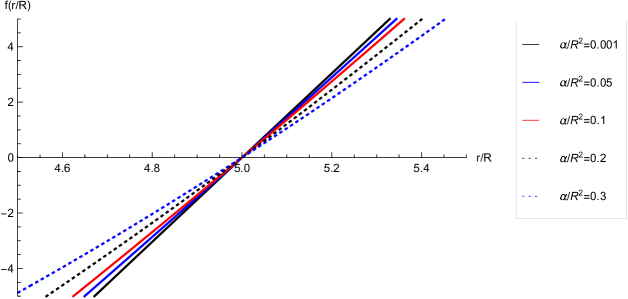
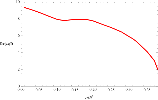
The black hole horizon corresponds to the largest root of . In Fig.1 we show the behavior of of different values of .
It is convenient to measure all the quantities in the units of the same dimension, so we express as a function of the event horizon :
| (5) |
where the cosmological constant can be expressed in terms of the AdS radius , which is defined by , as
| (6) |
III Scalar field perturbations
The QNMs of scalar perturbations in the background of the metric (4) are given by the scalar field solution of the Klein-Gordon equation
| (7) |
with suitable boundary conditions for a black hole geometry. In the above expression is the mass of the scalar field . Now, by means of the following ansatz
| (8) |
the Klein-Gordon equation reduces to
| (9) |
where represents the azimuthal quantum number and the prime denotes the derivative with respect to . Now, defining and by using the tortoise coordinate defined by , the Klein-Gordon equation can be written as a one-dimensional Schrödinger equation
| (10) |
with an effective potential , which is parametrically thought as , given by
| (11) |
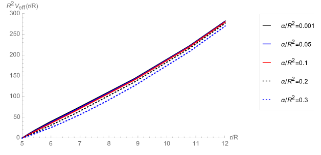
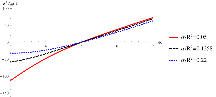
The effective potential diverges at spatial infinity and it is positive definite everywhere outside the event horizon, see Fig. 2. Therefore, we will consider as a boundary condition that the scalar field vanishes at the asymptotic region (Dirichlet boundary condition).
III.1 Scalar field stability with Dirichlet boundary condition
In order to know about the stability of the propagation of scalar fields, we follow a general argument given in Ref. Horowitz:1999jd . So, by defining
| (12) |
and inserting this expression in the Schrödinger like equation (10) yields
| (13) |
Then, multiplying Eq. (13) by and performing integrations by parts, and using the Dirichlet boundary condition for the scalar field at spatial infinity, one can obtain the following expression
| (14) |
In general, the QNFs are complex, where the real part represents the frequency of the oscillation and the imaginary part describes the rate at which this oscillation is damped, with the stability of the scalar field being guaranteed if the imaginary part is negative. The potential (5) is positive outside the horizon and then the left hand side of (14) is strictly positive, which demand that , and then we conclude that the stability of the propagation of a scalar field respecting Dirichlet boundary conditions is stable.
III.2 Numerical analysis
In this section we will solve numerically the differential equation (9) in order to compute the QNFs for the black hole described by the metric by using the pseudospectral Chebyshev method, see for instance Boyd . First, under the change of variable the radial equation (9) becomes
| (15) |
where the prime denotes derivative with respect to y. In the new coordinate the event horizon is located at and the spatial infinity at . Now, we consider the boundary conditions. In the neighborhood of the horizon (y 0) the function behaves as
| (16) |
Here, the first term represents an ingoing wave and the second represents an outgoing wave near the black hole horizon. Imposing the requirement of only ingoing waves on the horizon, we fix . On the other hand, at infinity the function behaves as
| (17) |
So, imposing the scalar field vanishes at infinity requires . Taking into account the above behaviors of the scalar field at the horizon and at spatial infinity we define
| (18) |
Then, by inserting this last expression in Eq. (15) we obtain an equation for the function , which we solve numerically employing the pseudospectral Chebyshev method. The solution for the function is assumed to be a finite linear combination of the Chebyshev polynomials, and it is inserted in the differential equation for . The interval is discretized at the Chebyshev collocation points. Then, the differential equation is evaluated at each collocation point. So, a system of algebraic equations is obtained, which corresponds to a generalized eigenvalue problem and it is solved numerically for .
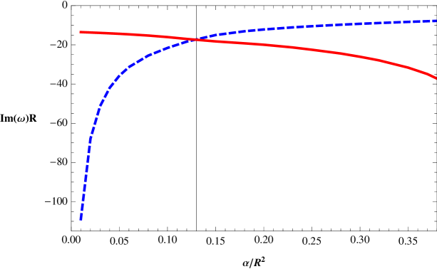
In Fig. 4, left panel, we show the behavior of the imaginary part of the QNFs for a massless scalar field with as a function of , for a ratio , and also we show the real part of the QNFs, under the same considerations, right panel. We can observe the existence of two branches, one of them, corresponds to the branch perturbative in (red continuous line) which consists of complex QNFs that in the limit , approximate to the QNFs of a massless scalar field in the background of the SAdS black hole, see Horowitz:1999jd . On the other hand, the branch nonperturbative in (blue dashed line) consists of purely imaginary QNFs, that diverge in the limit , therefore they do not exist for SAdS black hole. We show in Table 1 some numerical values of the QNFs. Also, we observe that the imaginary part of the QNFs is always negative for both branches; therefore, the propagation of massless scalar fields is stable in this background. It is worth to mention that there is a critical value , where the curves intersect and both branches have the same imaginary part, for lower than the critical value the nonperturbative branch decays faster than the perturbative branch, while that for greater than the critical value, the behavior is opposite, i.e., the pertubative branch decays faster than the nonperturbative branch, thus the nonperturbative branch dominates in this case. The real part of the perturbative QNFs, see Fig. 4, shows a smooth behavior and we observe that the frequency of the oscillation decreases when increases, in addition, we observe that there is a small range where the frequency increases slightly and then decreases again.
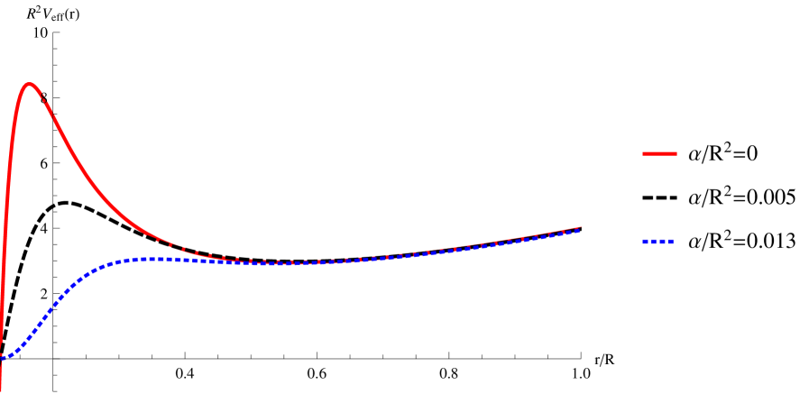
We observe that for there exist two different potentials 222We thank the referee for pointing out this behaviour of the potential to us. , one that looks like a potential barrier near the outside horizon-well-increasing, see Fig. 3, while the other is a monotonically increasing function like Fig. 2. The former shows a feature of small SAdS black hole, whereas the latter indicates a large SAdS black hole. In Myung:2008pr was showed that a potential-step type provides the purely imaginary QNFs, while the potential-barrier type gives the complex QNFs of a scalar field for the charged dilaton black hole. The presence of the bump near the horizon explains clearly why the QNFs for gravitational and electromagnetic perturbations of the small SAdS black hole are complex in Cardoso:2001bb . For the 4D Einstein-Gauss-Bonnet AdS black hole, we observe a similar behavior of the potential, for small black holes and small values of we note the presence of a potential barrier, which disappears when or increases, see Fig. 3. Thus, it is possible to explain the two kinds of QNFs of a scalar field around the 4D Einstein-Gauss-Bonnet AdS black holes by identifying their potentials, i.e., while the potential-barrier type gives the complex QNFs, the monotonically increasing type gives the purely imaginary QNFs. On the other hand, as mentioned, in Fig. 4 we observe that for the complex QNFs dominate, while that for the purely imaginary QNFs dominate. Interestingly, we found that this behavior is related to the change of concavity of the potential at the event horizon. We found that for the second derivative of the effective potential evaluated at the horizon is always negative, and it is given by
| (19) |
however, for , the concavity of the potential at the event horizon can be positive, and we note that the potential has a point of inflection, see Fig. 5, at the event horizon for where the curves in Fig. 4 intersect. For the potential has negative concavity at the event horizon, such as for the SAdS black hole, and the complex QNF dominates, while that for the concavity of the potential at the event horizon is positive and the purely imaginary QNF dominates. The change of the sign of when increases is attributed to the effect of the higher order curvature terms on the metric.
| Nonperturbative QNFs | Perturbative QNFs | |
|---|---|---|
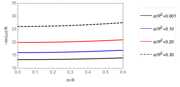
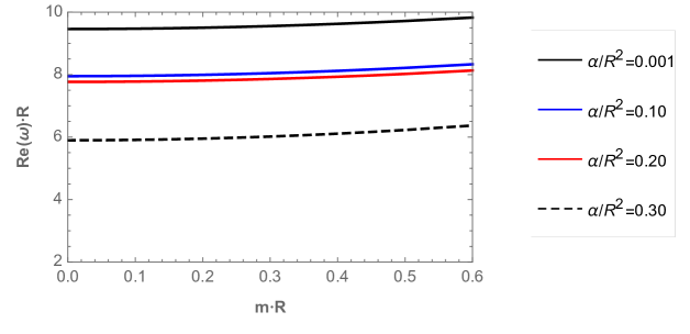
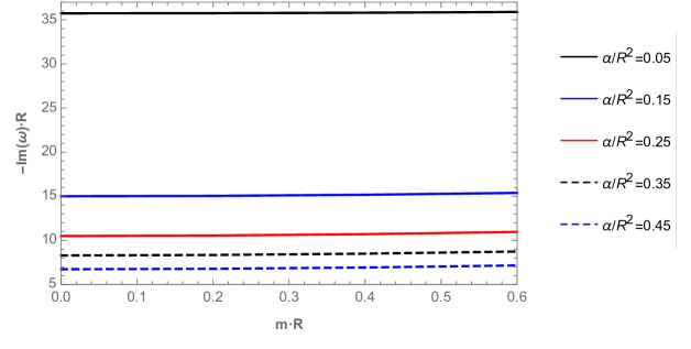
Now, in order to analyze the behavior of the QNFs of massive scalar field, we plot in Fig. 6, their behavior, for the lowest angular number as a function of , and for different values of . We can observe the complex branch (top panel) and the purely imaginary branch (bottom panel), which belong to the perturbative and nonperturbative branches, respectively. For the perturbative branch, we can observe that there is a faster decay rate of the perturbations when the mass of the scalar field increases, and the frequency of the oscillations increases too. Also, the decay rate and the frequency of the oscillation increases when decreases, for a fixed value of . On the other hand, for the nonperturbative branch the decay rate increases slightly when the scalar field mass increases. Also, the there is a faster decay when decreases.
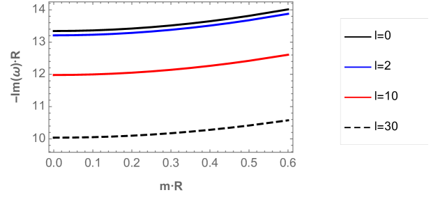
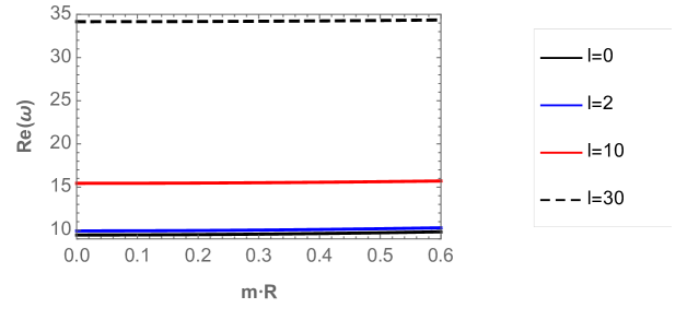
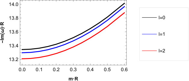
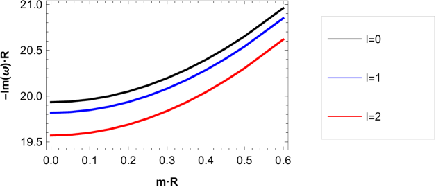
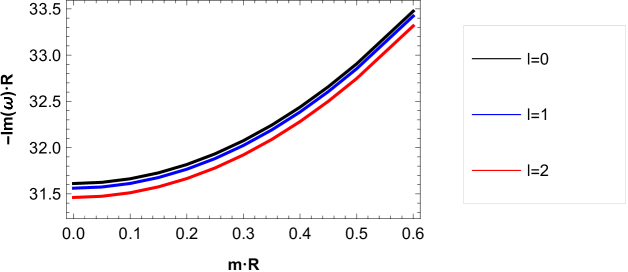
Now, in order to analyze the behavior of the QNFs of massive scalar field, we plot in Fig. 7, their behavior, for low angular numbers and high angular numbers as a function of with fixed. For the perturbative branch, we can observe that there is a lower decay rate and the frequency of the oscillations increases when the angular number increases. In Fig. 8, we observe that the behavior is similar for low angular numbers and different values of .
IV Conclusions
In this work, we considered 4D Einstein-Gauss-Bonnet black holes in AdS spacetime as backgrounds and we studied the propagation of probe scalar fields. We found numerically the quasinormal frequencies for different values of the Gauss-Bonnet coupling constant , the multipole number and the mass of the scalar field by using the pseudospectral Chebyshev method. Mainly, we found two branches of QNFs, a branch perturbative in the coupling constant , and another branch nonperturbative in , that is, they do not exist in the limit .
The branch nonperturbative in is characterized by purely imaginary QNFs with a faster decay when decreases, while that for the branch perturbative in the QNFs tend to the QNFs of the Schwarzschild AdS black hole when , and a lower decay is observed when decreases. Also, we found that the imaginary part of the QNFs is always negative for both branches; therefore, the propagation of scalar fields is stable in the asymptotically AdS 4D Einstein-Gauss-Bonnet black hole. There are two different behaviors of potential, one that looks like a potential barrier near the outside horizon-well-increasing, while the other is a monotonically increasing function. The former shows a feature of small SAdS black hole, whereas the latter indicates a large SAdS black hole. For small black holes and small values of we note the presence of a potential barrier, which disappears when or increases. Therefore, it is posible to explain the two kinds of QNFs of a scalar field around the 4D Einstein-Gauss-Bonnet AdS black holes by identifying their potentials, i.e., while the potential-barrier type gives the complex QNFs, the monotonically increasing type gives the purely imaginary QNFs.
Interestingly, we found that there is a critical value of , where both branches have the same imaginary part, and for values of lower than the critical value the nonperturbative branch decays faster than the perturbative branch, while that for values of greater than the critical value, the behavior is opposite, i.e., the pertubative branch decays faster than the nonperturbative branch, thus the nonperturbative branch dominates in this case. Additionally, we have found that for the second derivative of the effective potential evaluated at the horizon is always negative, while that for , the concavity of the potential at the event horizon can be positive, and we note that the potential has a point of inflection at the event horizon for . For the potential has negative concavity at the event horizon, such as for the SAdS black hole, and the complex QNF dominates, while that for the concavity of the potential at the event horizon is positive and the purely imaginary QNF dominates. The change of sign of the second derivative of the effective potential evaluated at the horizon when increases is attributed to the effect of the higher order curvature terms on the metric.
We showed that the phenomena of nonperturbative modes arises for scalar field perturbations for the 4D Einstein-Gauss-Bonnet theory, by extending the presence of nonperturbative modes to other theory. On the other hand, the inverse of the imaginary part of the fundamental quasinormal frequency is related, through the AdS/CFT duality, to the thermalization time of the quantum states in the boundary field theory Horowitz:1999jd . In addition, it was found in Grozdanov:2016fkt ; Grozdanov:2016vgg that black holes with AdS asymptotics in theories with higher curvature terms can help to describe the intermediate t’Hooft coupling in the dual field theory ; thus, we hope that the results obtained in this work can have applications along this line.
Acknowledgements.
We would like to thank the referee for his/her careful review of the manuscript and his/her valuable comments and suggestions which helped us to improve the manuscript considerably. Y.V. acknowledge support by the Dirección de Investigación y Desarrollo de la Universidad de La Serena, Grant No. PR18142.References
- (1) D. Glavan and C. Lin, Phys. Rev. Lett. 124, no. 8, 081301 (2020) [arXiv:1905.03601 [gr-qc]].
- (2) P. G. S. Fernandes, arXiv:2003.05491 [gr-qc].
- (3) S. G. Ghosh and R. Kumar, arXiv:2003.12291 [gr-qc].
- (4) D. V. Singh, S. G. Ghosh and S. D. Maharaj, arXiv:2003.14136 [gr-qc].
- (5) S. W. Wei and Y. X. Liu, arXiv:2003.07769 [gr-qc].
- (6) A. Kumar and R. Kumar, arXiv:2003.13104 [gr-qc].
- (7) R. A. Konoplya and A. Zhidenko, arXiv:2003.12171 [gr-qc].
- (8) R. A. Konoplya and A. Zhidenko, Phys. Rev. D 101, no. 8, 084038 (2020) [arXiv:2003.07788 [gr-qc]].
- (9) R. A. Konoplya and A. Zhidenko, arXiv:2005.02225 [gr-qc].
- (10) K. Hegde, A. Naveena Kumara, C. L. A. Rizwan, A. K. M. and M. S. Ali, arXiv:2003.08778 [gr-qc].
- (11) S. A. Hosseini Mansoori, arXiv:2003.13382 [gr-qc].
- (12) S. W. Wei and Y. X. Liu, arXiv:2003.14275 [gr-qc].
- (13) D. V. Singh and S. Siwach, arXiv:2003.11754 [gr-qc].
- (14) B. Eslam Panah and K. Jafarzade, arXiv:2004.04058 [hep-th].
- (15) C. Y. Zhang, P. C. Li and M. Guo, arXiv:2003.13068 [hep-th].
- (16) R. A. Konoplya and A. F. Zinhailo, arXiv:2004.02248 [gr-qc].
- (17) R. A. Konoplya and A. F. Zinhailo, arXiv:2003.01188 [gr-qc].
- (18) R. A. Konoplya and A. Zhidenko, arXiv:2003.12492 [gr-qc].
- (19) A. K. Mishra, arXiv:2004.01243 [gr-qc].
- (20) M. S. Churilova, arXiv:2004.00513 [gr-qc].
- (21) C. Y. Zhang, S. J. Zhang, P. C. Li and M. Guo, arXiv:2004.03141 [gr-qc].
- (22) M. Guo and P. C. Li, arXiv:2003.02523 [gr-qc].
- (23) M. Heydari-Fard, M. Heydari-Fard and H. Sepangi, [arXiv:2004.02140 [gr-qc]]
- (24) R. Roy and S. Chakrabarti, [arXiv:2003.14107 [gr-qc]].
- (25) C. Liu, T. Zhu and Q. Wu, arXiv:2004.01662 [gr-qc].
- (26) M. Gurses, T. C. Sisman and B. Tekin, arXiv:2004.03390 [gr-qc].
- (27) S. Mahapatra, arXiv:2004.09214 [gr-qc].
- (28) F. W. Shu, arXiv:2004.09339 [gr-qc].
- (29) S. X. Tian and Z. H. Zhu, arXiv:2004.09954 [gr-qc].
- (30) H. Lu and Y. Pang, arXiv:2003.11552 [gr-qc].
- (31) P. G. S. Fernandes, P. Carrilho, T. Clifton and D. J. Mulryne, arXiv:2004.08362 [gr-qc].
- (32) R. A. Hennigar, D. Kubiznak, R. B. Mann and C. Pollack, arXiv:2004.09472 [gr-qc].
- (33) R. B. Mann and S. F. Ross, Class. Quant. Grav. 10, 1405 (1993) [gr-qc/9208004].
- (34) T. Kobayashi, arXiv:2003.12771 [gr-qc].
- (35) B. P. Abbott et al. [LIGO Scientific and Virgo Collaborations], Phys. Rev. Lett. 116, no. 6, 061102 (2016)
- (36) T. Regge and J. A. Wheeler, Phys. Rev. 108, 1063 (1957).
- (37) F. J. Zerilli, Phys. Rev. D 2, 2141 (1970).
- (38) K. D. Kokkotas and B. G. Schmidt, Living Rev. Rel. 2, 2 (1999) [gr-qc/9909058].
- (39) H. P. Nollert, Class. Quant. Grav. 16, R159 (1999).
- (40) R. A. Konoplya and A. Zhidenko, Rev. Mod. Phys. 83, 793 (2011) [arXiv:1102.4014 [gr-qc]]; E. Berti, V. Cardoso and A. O. Starinets, Class. Quant. Grav. 26, 163001 (2009) [arXiv:0905.2975 [gr-qc]]; K. D. Kokkotas and B. G. Schmidt, Living Rev. Rel. 2, 2 (1999) [gr-qc/9909058].
- (41) B. P. Abbott et al. [LIGO Scientific and Virgo Collaborations], Phys. Rev. Lett. 116, no. 22, 221101 (2016)
- (42) R. Konoplya and A. Zhidenko, Phys. Lett. B 756, 350 (2016)
- (43) P. A. Gonzalez, R. A. Konoplya and Y. Vasquez, Phys. Rev. D 95, no. 12, 124012 (2017) [arXiv:1703.06215 [gr-qc]].
- (44) S. Grozdanov, N. Kaplis and A. O. Starinets, JHEP 1607, 151 (2016) [arXiv:1605.02173 [hep-th]].
- (45) R. A. Konoplya and A. Zhidenko, Phys. Rev. D 95, no. 10, 104005 (2017) [arXiv:1701.01652 [hep-th]].
- (46) P. A. Gonzalez, Y. Vasquez and R. N. Villalobos, Phys. Rev. D 98, no. 6, 064030 (2018) [arXiv:1807.11827 [gr-qc]].
- (47) S. Grozdanov and A. O. Starinets, arXiv:1611.07053 [hep-th].
- (48) T. Takahashi and J. Soda, Prog. Theor. Phys. 124, 911 (2010) [arXiv:1008.1385 [gr-qc]].
- (49) G. Dotti, R. J. Gleiser, Phys. Rev. D 72, 044018 (2005) [gr-qc/0503117].
- (50) R. J. Gleiser, G. Dotti, Phys. Rev. D 72, 124002 (2005) [gr-qc/0510069].
- (51) J. P. Boyd, Chebyshev and Fourier Spectral Methods. Dover Books on Mathematics. Dover Publications, Mineola, NY, second ed., 2001.
- (52) S. I. Finazzo, R. Rougemont, M. Zaniboni, R. Critelli and J. Noronha, JHEP 1701, 137 (2017) [arXiv:1610.01519 [hep-th]].
- (53) P. A. González, E. Papantonopoulos, J. Saavedra and Y. Vásquez, Phys. Rev. D 95, no. 6, 064046 (2017) [arXiv:1702.00439 [gr-qc]].
- (54) R. G. Cai, L. M. Cao and N. Ohta, JHEP 1004, 082 (2010) [arXiv:0911.4379 [hep-th]].
- (55) G. Cognola, R. Myrzakulov, L. Sebastiani and S. Zerbini, Phys. Rev. D 88, no. 2, 024006 (2013) [arXiv:1304.1878 [gr-qc]].
- (56) G. T. Horowitz and V. E. Hubeny, Phys. Rev. D 62, 024027 (2000) [hep-th/9909056].
- (57) Y. S. Myung, Y. W. Kim and Y. J. Park, Eur. Phys. J. C 58, 617 (2008) [arXiv:0809.1933 [gr-qc]].
- (58) V. Cardoso and J. P. S. Lemos, Phys. Rev. D 64, 084017 (2001) [gr-qc/0105103].
- (59) J. Chan and R. B. Mann, Phys. Rev. D 55 (1997), 7546-7562 [arXiv:gr-qc/9612026 [gr-qc]].
- (60) Y. Tomozawa, arXiv:1107.1424 [gr-qc].