PET Image Reconstruction with Multiple Kernels and Multiple Kernel Space Regularizers
Abstract
Kernelized maximum-likelihood (ML) expectation maximization (EM) methods have recently gained prominence in PET image reconstruction, outperforming many previous state-of-the-art methods. But they are not immune to the problems of non-kernelized MLEM methods in potentially large reconstruction error and high sensitivity to iteration number. This paper demonstrates these problems by theoretical reasoning and experiment results, and provides a novel solution to solve these problems. The solution is a regularized kernelized MLEM with multiple kernel matrices and multiple kernel space regularizers that can be tailored for different applications. To reduce the reconstruction error and the sensitivity to iteration number, we present a general class of multi-kernel matrices and two regularizers consisting of kernel image dictionary and kernel image Laplacian quatradic, and use them to derive the single-kernel regularized EM and multi-kernel regularized EM algorithms for PET image reconstruction. These new algorithms are derived using the technical tools of multi-kernel combination in machine learning, image dictionary learning in sparse coding, and graph Laplcian quadratic in graph signal processing. Extensive tests and comparisons on the simulated and in vivo data are presented to validate and evaluate the new algorithms, and demonstrate their superior performance and advantages over the kernelized MLEM and other conventional methods.
Keywords: PET image reconstruction, regularized MLEM, multiple kernels, dictionary learning, graph Laplacian quadratic.
1 Introduction
The maximum-likelihood (ML) expectation maximization (EM) and the maximum a posteriori (MAP) expectation maximization are two popular classes of methods for PET image reconstruction [1]. They both use EM to iteratively approximate ML or MAP probability.
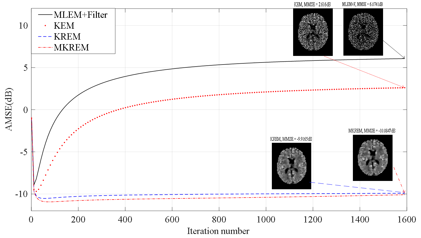
As exemplified in Fig. 1 (solid curve), the MLEM method has two main problems: its reconstruction error may decrease and then increases rapidly with iterations first, then slowly converges to very noisy images due to ML’s inherent nature of large variance under noise [1, 2]. These problems become more severe in the low count situation. Hence, MLEM’s iterated estimates must be stopped well before convergence and filtered for useable images. To overcome these problems, the MAPEM method was introduced in PET image reconstruction [1, 3, 4, 5]. This method is equivalent to a regularized MLEM estimation with the regularization functions (regularizers) introduced as the priors of PET images [3]. Thanks to regularization, MAPEM’s reconstruction error is much lower and its iterated estimates tend to converge much faster than its ML counterpart.
Because of its good numerical properties and convenience of incorporating priors, the MAPEM method, also known as Bayesian method, has been exploited in PET image reconstruction to incorporate various prior information, especially the anatomical priors from multi-modality imaging scanners, eg magnetic resonance (MR) image priors in PET-MR. This has led to numerous reconstruction algorithms with significant improvement of PET image quality and numerical robustness for various applications of different imaging conditions, see [6, 7, 8, 9, 10, 11, 12, 13] for examples.
Besides the MAPEM method, there are also other effective methods to introduce the priors in PET image reconstruction, eg the methods of joint and synergistic reconstruction of PET and MR images [14, 15, 16]. One of these methods is the kernelized expectation maximization (KEM) method recently introduced in [17, 18]. This method uses the prior data, such as MR anatomical images, to construct the kernel matrix and uses MLEM in the kernel space to iteratively estimate the kernel coefficients of the image, which in turn are mapped by the kernel matrix to the reconstructed image. It has shown superior performance in enhancing the spatial and temporal resolution and quantification in static and dynamic PET imaging, with great potential in low dose PET imaging. Following these promising results, a number of kernelized methods have recently been presented for various PET image reconstruction problems, see eg [21, 22, 23, 24, 25, 26, 27].
Despite the advantages of kernelized methods, they may suffer from the same problems of MLEM method. Fig. 1 (dotted curve) shows an example of high-count static PET image reconstruction using KEM, and similar result is also given in [20]. It can be seen that KEM behaves similarly to MLEM and can be highly sensitive to the iteration number around its minimum reconstruction error. This can be even worse in low-count situation. Such sensitivity may severely degrade PET image quality, since it is generally difficult in practice to preset the maximum iteration number to the optimal value with the minimum reconstruction error, see Section 3 for examples.
The reason for kernelized methods’ sensitivity to iteration number is the lack of effective regularization in their kernel space ML estimation. From the kernel and regularization theory [28], an optimization regularizer is generally a function of the optimizers (optimization variables) that varies with the optimizers, eg grows as the optimizers grow, so as to constrain the optimizers, and a kernel can function as a regularizer if it has the same property. This is the case in the MAPEM based reconstruction methods, eg [1, 3, 4, 5], where the regularizers are the functions of the estimated variables. Hence, they generally behave like the dashed and dashed-dotted curves in Fig. 1, with much lower reconstruction error and sensitivity to iteration number. But this is not the case in the kernelized methods, where the only possible regularizer, the kernel matrix, is constructed using prior data and does not vary with the estimated variables. Therefore, they generally lack effective regularization even though their kernel may be correlated with the estimated variables to some extent. For dynamic PET imaging, [20] has shown by simulations that KEM’s sensitivity can be reduced by combining the spatial kernel with a temporal kernel. However, without supporting mathematical theory, the underlying mechanism and generality of this KEM variant are unclear. Moreover, this variant is inapplicable to static PET imaging where no temporal kernel is available. All these strongly suggest that some explicit and effective regularizations are needed in the kernelized methods in order to reduce their reconstruction error and sensitivity to iteration number.
The kernelized method was initially proposed to use only a single spatial kernel, and was later extended to include another temporal kernel or spatial kernel from other source for improved performance [20, 19]. However, these extensions are application specific and have not provided a general guidance for finding suitable kernels for different applications.
To address above problems, we propose in this work a novel framework for the kernelized PET image reconstruction. This framework is a general reformulation of kernel space MAPEM estimation with multi-kernel matrices and multiple kernel space regularizers that can be tailored to application requirements. To significantly reduce the reconstruction error and sensitivity to iteration number, we present a general class of multi-kernel matrices and two specific kernel space regularizers, and use them to derive the single-kernel regularized EM (KREM) and multi-kernel regularized EM (MKREM) algorithms for PET image reconstruction. These algorithms are derived using the technical tools of multiple kernel combination in machine learning [30, 32, 31], image dictionary learning [33] in sparse coding, and graph Laplcian quadratic [34] in graph signal processing. We further use simulated and in vivo data to validate and evaluate the performance of KREM and MKREM, and demonstrate their superior performance and advantages over the existing methods by comprehensive comparisons.
This paper is organized as follows. Section 2 presents our proposed method in detail. Section 3 presents the simulation studies and comparisons of the proposed method with the existing methods. Section 4 presents the in vivo data testing results of the proposed method and compares with those of the existing methods. Discussions and Conclusions are presented in Sections 5 and 6, respectively.
2 Theory and Method
2.1 PET Image Reconstruction with Multi-regularizers
Let be the PET projection data vector with its elements being Poisson random variables having the log-likelihood function [18]
| (1) |
where is the total number of lines of response and is the expectation of . The expectation of , , is related to the unknown emission image by the forward projection
| (2) |
where is the th voxel intensity of the image , is the total number of voxels, is the PET system matrix, and is the expectation of random and scattered events.
An estimate of the unknown image can be obtained by the maximum a posteriori (MAP) estimation of [4, 1]
| (3) |
Here is a normalizing constant independent of ; represents the prior knowledge of unknown image and is assumed to have the Gibbs distribution [29]
| (4) |
where is a normalizing constant and the energy function. In this paper, we consider as a weighted sum of multiple prior functions
| (5) |
with the weighting parameters .
Solving from (3) is equivalent to maximizing the log-posterior probability with
| (6) |
where is as defined in (1), and the contributions of and have been excluded since they are independent of . When all , (6) reduces to the ML estimation [18]. The multiple prior functions in introduce multiple regularizers in the ML estimation.
2.2 PET Image Reconstruction with Single-kernel and Multi-Regularizers
Using the kernel theory [30], the unknown emission image can be presented in the kernel space as [18]
| (8) |
where is a kernel (basis) matrix and is the coefficient vector of under .
The th element of is given by , where is a kernel (function), and are respectively the data vectors for the th and th elements of in the training dataset of obtained from other sources, eg MR anatomical images of the same (class of) subject/s, is a nonlinear function mapping to a higher dimensional feature space but needs not to be explicitly known, and denotes the inner product.
Typical kernels include the radial Gaussian kernel and the polynomial kernel
| (9) |
| (10) |
where , and are kernel parameters, and is the 2-norm of a vector. For computation simplicity and performance improvement, the kernel matrix in practice is often constructed using
| (11) |
where is the neighborhood of the th element of emission image , with the neighborhood size . Other methods such as (the nearest neighbor) of , measured by , can also be used [18].
Because the kernel matrix constructed in (11) involves only a single kernel , we will call it the single-kernel matrix hereafter.
Using the kernel space image model (8), we can convert the forward projection (2) and the log-posterior probability maximization (6) to their respective kernel space equivalents
| (12) |
| (13) |
and obtain a single-kernel regularized EM (KREM) algorithm
| (14) | |||
where with absorbed into its parameters. We can then use (14) to estimate the coefficient and use to obtain an estimate of the image .
The KREM algorithm (14) includes the KEM algorithm of [18, 20] as a special case when all . As shown in Sections 3 and 4, the KEM algorithm tends to have larger reconstruction error and is sensitive to the number of iterations and the neighborhood size used in (11) to construct the single-kernel matrix . These problems may significantly degrade KEM’s performance in PET image reconstruction, especially at the low counts. Whereas, the KREM algorithm (14) with regularizations can effectively overcome these problems.
2.3 PET Image Reconstruction with Multi-kernels and Multi-Regularizers
The single-kernel matrix in (14) is the core of KREM algorithm. Its effect can be tuned by the selection of kernel , kernel parameters, and neighborhood size in (11). However, the efficacy of such tuning is limited as a single kernel is often insufficient for complex problems, such as heterogeneous data [31]. To solve this problem, a multi-kernel approach has been developed in machine learning, which combines multiple base kernels, such as that of (9) or (10), to construct more complex kernel and corresponding multi-kernel matrix for significantly improved performance [32, 31].
Inspired by the success of multi-kernel approach in machine learning, we introduce this approach in PET image reconstruction. We construct the multi-kernel matrix by
| (15) | |||
and replace the single-kernel matrix with in KREM algorithm (14) to derive the multi-kernel KREM (MKREM) algorithm for improved performance.
In (15), , , are constructed using (11) with different or same having different or same parameters and neighborhood size for different ; and , , is the product of ’s thus constructed.
The multi-kernel matrix constructed using (15) includes single-kernel matrix as a special case when . Hence, the MKREM algorithm derived from replacing by in (14) includes KREM algorithm as a special case. We therefore call (14) the MKREM algorithm and KREM algorithm alternately when there is no confusion.
2.4 Kernel Space Image Dictionary Regularizer
The regularizers in (14) are symbolic. In this and the next subsections, we will present two specific regularizers to be used in this work. To facilitate presentation, we introduce the kernel space image dictionary for PET emission image .
Let , , , be two groups of single-kernel matrices constructed using (11) with the kernel and neighborhood size for and for . Let , be two multi-kernel matrices constructed using (15) with for and for . Here is used as in MKREM algorithm (14) and is used in the dictionary learning described below. When , and reduce to the single-kernel matrices. As shown by the experiment results in Section 3, and hence are generally needed for the best reconstruction performance.
Since , and , admits the kernel matrix factorization
| (16) |
Replacing in (8) by and respectively gives the representations of emission image under the multi-kernel matrices and
where are respectively the coefficient vectors of under and and are related by .
The and can be viewed as kernel space image signals and hence both admit dictionary representation [33]. Defining a dictionary with dictionary atoms and a coefficient vector for , we can represent and respectively as
where is a dictionary for . It can be seen that is a mapping of and in the kernel space of to and in the kernel space of .
Let be the matrix consisting of training data vectors for , obtained from other sources, eg MR anatomical images of the same (class of) subject/s. We use the following sparse dictionary learning to obtain the dictionary [33]
| (17) |
where is the data matrix for dictionary learning, is the matrix consisting of estimates of the coefficient vector , is the Frobenius norm, and is a sparsity constraint constant. Theoretically, is always positive semidefinite [30]. In the rare case it is singular, , with a small constant, can be used as without affecting image reconstruction result.
In case the number of training data vectors is limited, eg , or the row dimension of is too high, we can use the patch-based dictionary learning to increase training data or reduce computation complexity [33]
| (18) |
where is the operator extracting patches from and .
A number of well developed methods can be used to solve (17) ((18)) for and [33]. All these methods are based on the alternating optimization: 1) fix and solve (17) ((18)) for , 2) fix and solve (17) ((18)) for , 3) repeat 1) and 2) until the maximum number of iterations is reached. In this work, we use the orthogonal matching pursuit (OMP) in 1) to compute and the K-SVD in 2) to compute [33].
With above learned dictionary , we can obtain
| (19) |
and introduce the first regularizer and its derivative
| (20) |
| (21) |
where is from the th MKREM iteration in (14), and is from solving the optimization below for using and OMP before the th MKREM iteration.
| (22) |
2.5 Kernel Space Graph Laplacian Quadratic Regularizer
As mentioned above, the neighborhood size is generally needed for the multi-kernel matrix used in dictionary learning. This is to allow the dictionary to capture the local texture details embedded in the training image data which is usually the images with anatomical details. To avoid over-localization of the image reconstruction, we treat the image data as the signal on graph and use the graph Laplacian quadratic [34] of the estimated kernel image , given in (23), as the second regularizer to smooth the estimated PET image on the image graph at each iteration of MKREM algorithm (14).
| (23) |
with the derivative
| (24) |
where and is the Laplacian matrix of the graph of training image data described below.
Inspired by [35], we treat a training image as a graph signal and construct its Laplacian matrix as follows: We first use a window of size centered at the th element of to extract elements and use them to form the vector , for . Then we construct a distance matrix with elements , , and convert to an affinity matrix by an adaptive Gaussian function , where is the () smallest in the th row of . Next, we symmetrize to and construct a Markov transition matrix with . If there are training images available, we apply above procedure to each image to get and take .
Using above constructed , we construct the Laplacian matrix where is identity matrix and is the optimal Markov transition matrix. The optimal power of is determined by with a small constant, and as described above.
2.6 Proposed Method
Substituting and derived in (21) and (24) into (14), we obtain the full mathematical expression of MKREM algorithm proposed for PET image reconstruction
| (25) | |||
where has replaced in (14) as explained in Subsection 2.4. When is constructed with in (15), it reduces to a single-kernel matrix and (25) becomes the full mathematical expression of KREM algorithm (14). The pseudo-code of the proposed method is given in Algorithm 1.
3 Simulation studies
To investigate their behavior and performance, we have applied the proposed MKREM and KREM algorithms to the simulated low count and high count sinogram data to reconstruct the PET images and compare them with the existing PET image reconstruction algorithms. Since the KEM algorithm [18] has proven to be superior to many state-of-the-art PET image reconstruction algorithms, we have mainly compared the MKREM, KREM and KEM algorithms. We have also compared with MLEM with Gaussian filter (MLEM+F) to show some common problems of PET image reconstruction methods that are based on the un-regularized EM.
3.1 PET and Anatomical MRI Data Simulation
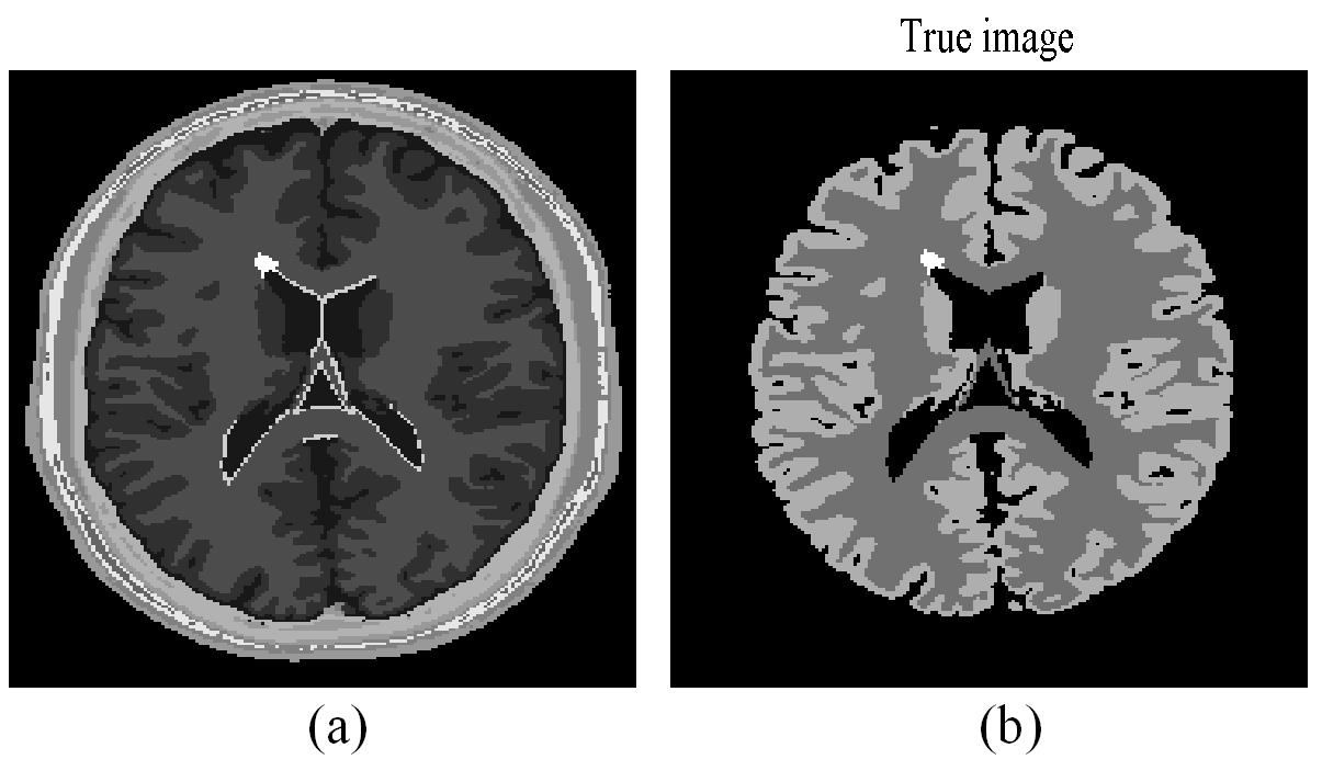
The same method as that of [18] was used to generate 3D PET activity images. The 3D anatomical model from BrainWeb database consisting of 10 tissue classes was used to simulate the corresponding PET images [36],[37]. The regional time activities at 50 minutes were assigned to different brain regions to obtain the reference PET image. The matching T1-weighted 3D MR image generated from BrainWeb database was used as training image data. A slice of the anatomical model and the reference PET image are shown in Fig. 2 (a) and (b), respectively. The bright spot in the periventricular white matter is a simulated lesion created by BrainWeb.
The reference PET image was forward projected to generate noiseless sinograms using the PET system matrix generated by Fessler toolbox. The count number of noiseless sinograms was then set to 370k and 64k, respectively, to obtain the noiseless high count sinograms and the noiseless low count sinograms. The thinning Poisson process was applied to the noiseless high count and low count sinograms to generate the noisy high count and noisy low count sinograms for image reconstruction tests. Attenuation maps, mean scatters and random events were included in all reconstruction methods to obtain quantitative images. Ten noisy realizations were simulated and each was reconstructed independently for comparison.
To simulate the real scanning process and test the robustness of different methods, the BrainWeb generated MR images with noise were used as the training data to construct the kernel matrices, dictionaries and Laplacian matrix of the proposed MKREM and KREM methods.
3.2 Algorithms Setup and Performance Metrics
We used , , for and , for in (15) to construct the multi-kernel matrices for the MKREM algorithm (14) and for dictionary learning. The above single-kernel matrices and were constructed using the Gaussian kernel (9) with , and in (11). The thus constructed was used as the kernel matrix in the KREM algorithm (14).
For kernel space dictionary learning, the training data was divided into 12960 overlapping 5 5 patches. To ensure the generalization and efficiency of learned dictionary, 400 patches were randomly chosen from the 12960 patches. The matrix of patched training data was . The number of dictionary atoms was set to 50 to obtain over-complete dictionaries and . The sparsity constraint constant and the total iteration number = 50 were used in dictionary learning.
The data window of size was used to construct the Markov transition matrix , and was used to find the optimal for the Laplacian matrix .
For the low count image reconstruction, we tuned the weighting parameters to and , and for the high count image, and .
The same as described above was used as the kernel matrix for the KEM algorithm. The post-filter of MLEM was Gaussian filter with window size 55.
For fair comparison, the total iteration numbers and parameters of the compared methods were tuned separately to achieve their respective minimum mean square error (MMSE) in image reconstruction.
The mean square error (MSE), , the ensemble mean square bias, , and the standard deviation, , were used for the quantitative performance evaluation and comparison of the algorithms, where is the th element of reconstructed PET image, is the th element of the reference PET image (the true image) and is the total number of noisy realizations.
3.3 Image Reconstruction Performance
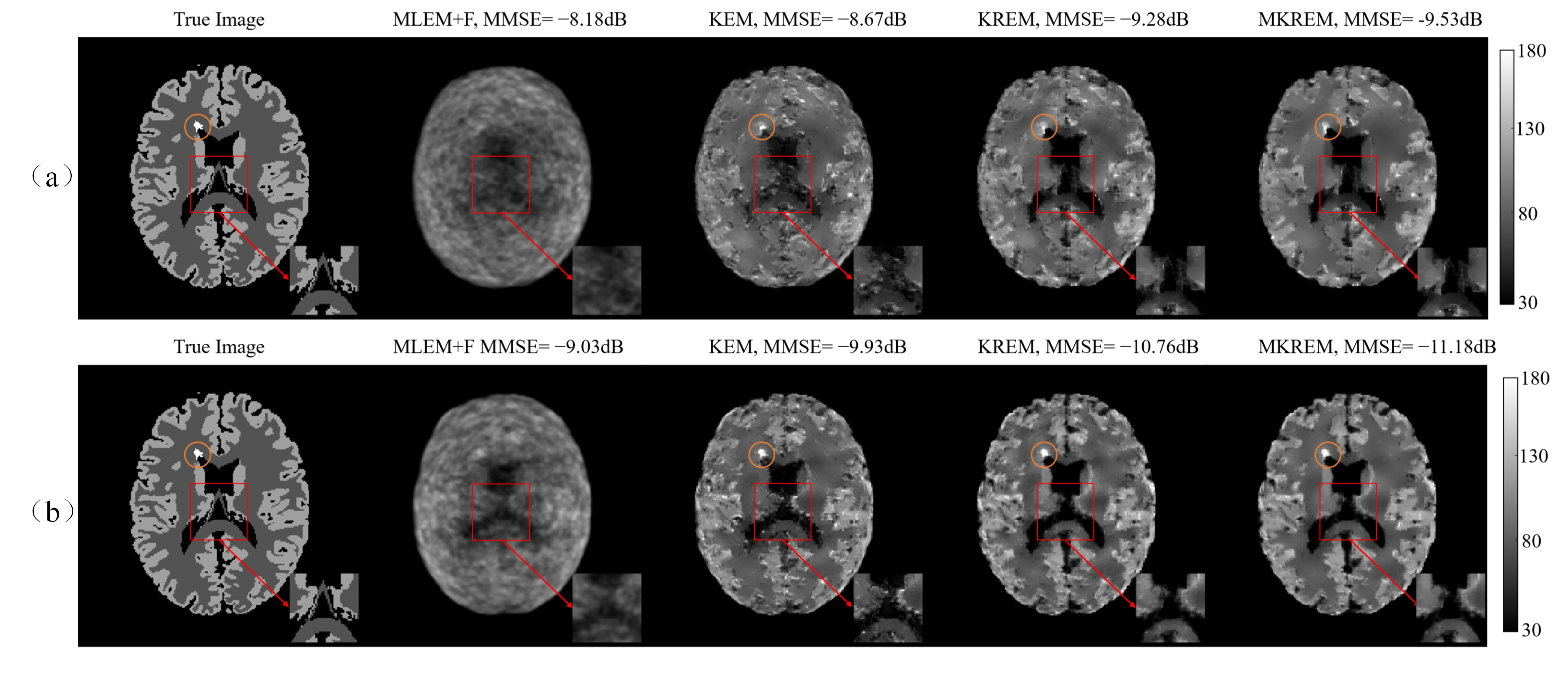
Fig. 3(a) shows the true image and the images reconstructed by different algorithms for the slice of low count image. As seen from the figure, KREM and MKREM achieve lower MMSE and better visual effects than those of MLEM+F and KEM, and the KREM and MKREM images appear to be less noisy, higher contrast and clearer texture. The intensity (brightness) of the lesion area in KREM and MKREM images, especially that of MKREM images, is closer to the true image than in KEM and MLEM images. As shown in the enlarged cutouts, the edges and texture of the true image are better preserved by KREM and MKREM than by MLEM+F and KEM.
Fig. 3(b) shows the true image and the images reconstructed by different algorithms for the same slice of high count image. Due to the high count of this image, all algorithms achieve better results. But KREM and MKREM images are sharper and less noisy with lower MMSE and globally clearer image details than MLEM+F and KEM images. The lesion area in KREM and MKREM images is more pronounced than in MLEM+F and KEM images. The quantitative comparison is given in Fig. 4. As shown in the enlarged cutouts, KREM and MKREM can more effectively preserve the boundaries and details of the image than MLEM+F and KEM.
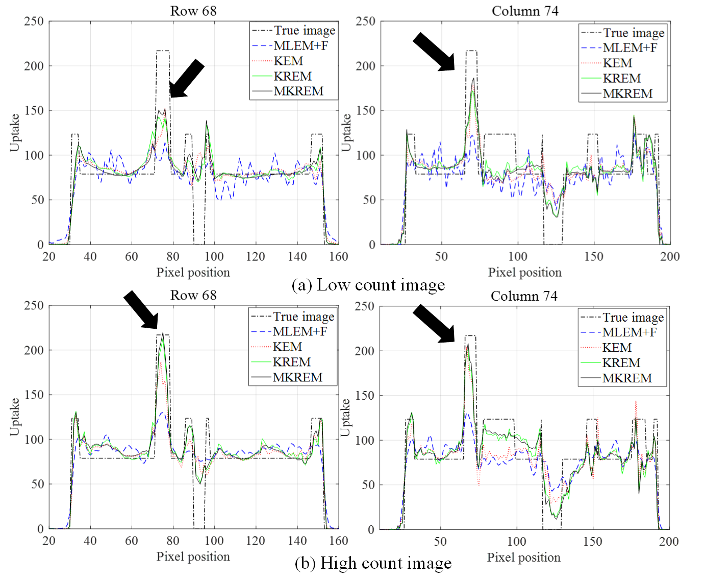
Fig. 4 plots the pixel line profiles across the lesion in the low count and high count images. The lesion area shows up as one peak indicated by the black arrow, which is significantly different from the white matter region in the high count image. Compared with other three methods, MKREM has the highest uptake in the lesion area in both low count and high count images.
The above results show that KREM and MKREM outperforms MLEM+F and KEM for both low count and high count images in terms of image visual effect and reconstruction MMSE.
Comparing the results in Fig.’s 3-4, it can be clearly seen that MKREM further outperforms KREM in image reconstruction MMSE, image visual effects and pixel uptakes for the low count and high count images.
3.4 Average MSE, Convergence Speed and Robustness
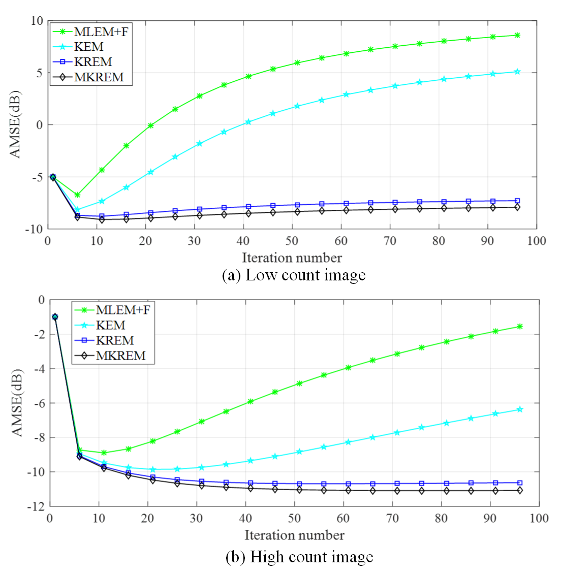
Fig. 5 plots the average MSE (AMSE) versus the iteration number of MLEM+F, KEM, KREM and MKREM over ten noisy realizations. As seen from the plotted curves, all these algorithms approach their respective minimum AMSE’s rather quickly as the iteration number increases, but the minimum AMSE’s of KREM and MKREM are lower than those of MLEM+F and KEM, and that of MKREM is the lowest. When the iteration number further increases to beyond the minimum AMSE points, the AMSE’s of MLEM+F and KEM start to increase rapidly. As shown before in Fig. 1, such increase can last thousands iterations before the AMSE’s slowly converge to some very high values, resulting in extremely noisy and useless images. The same phenomenon has been observed and analyzed in [2] for non-kernelized MLEM in PET image reconstruction, and it is shown now for KEM in the same application. In stark contrast, the AMSE’s of KREM and MKREM are quite stable, with negligible increases from their minimum AMSE’s over thousands iterations. As shown in Fig. 5, these results hold for both low count and high count cases.
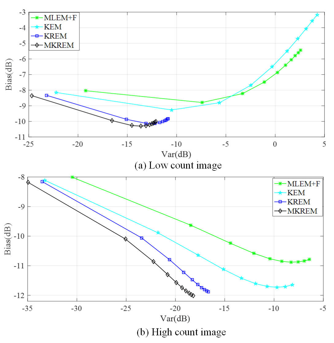
Fig. 6 shows the ensemble mean squared bias versus mean variance trade-off of different algorithms at the iterations 3 to 93 in increments of 10. As seen from the figure, the proposed KREM and MKREM always get much lower bias and variance simultaneously than those of MLEM+F and KEM for both low count and high count images.
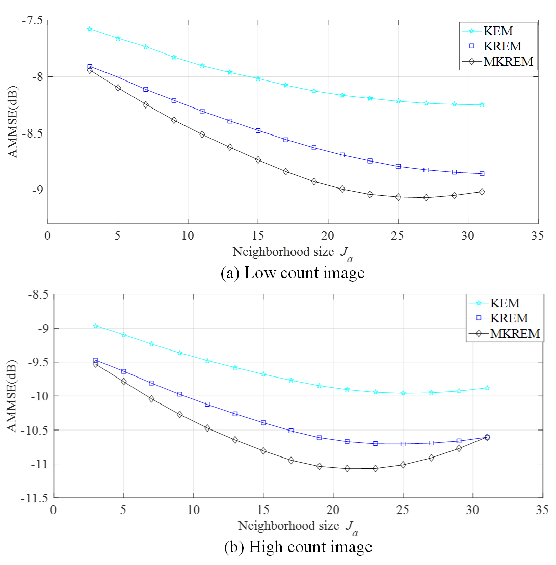
Fig. 7 shows the AMMSE’s of KEM, KREM and MKREM versus the neighborhood size over ten noisy realizations. As seen from the figure, in both the low count and high count cases, KREM and MKREM achieve much lower AMMSE than that of KEM over a wide range of selections, and MKREM achieves the lowest. Hence, KREM and MKREM are less sensitive to the selection of .
4 Tests on In-vivo Data
To validate the results of simulation studies and further compare the performance of MLEM+F, KEM, KREM and MKREM methods, we have applied them to in-vivo phantom and human data. The PET in-vivo phantom and human data and corresponding MR images were acquired from a Siemens (Erlangen) Biograph 3 Tesla molecular MR (mMR) scanner. The MR data were acquired with a 16-channel RF head coil, and the human PET data were acquired with an average dose 233MBq of [18-F] FDG infused into the subject over the course of the scan at a rate of 36mL/hr [38]. The raw data for a particular time image was rebinned into sinograms, with 157 angular projections and 219 radial bins, for PET image reconstruction; and the corresponding MR image was used as training data for constructing the kernel and Laplacian matrices and dictionary learning.
To reconstruct PET images with better quality, we used manufacturer software to evaluate correction factors for random scatters, attenuation and detector normalization, and used these in the reconstruction process of all methods.
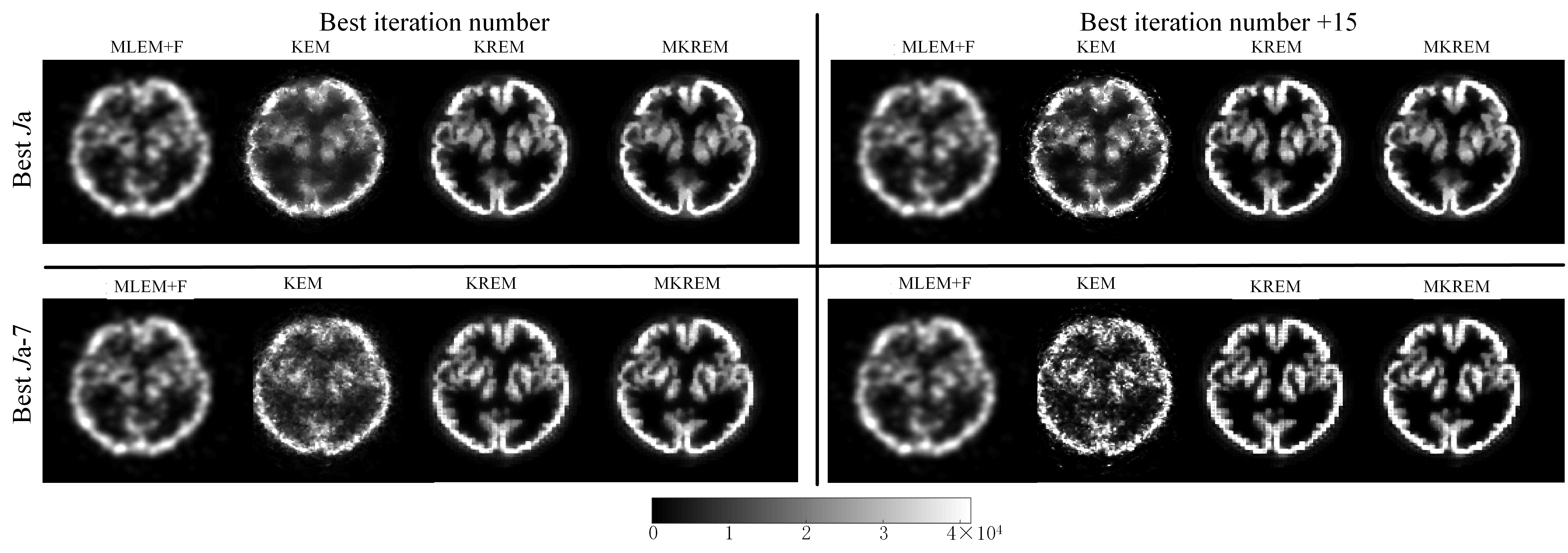
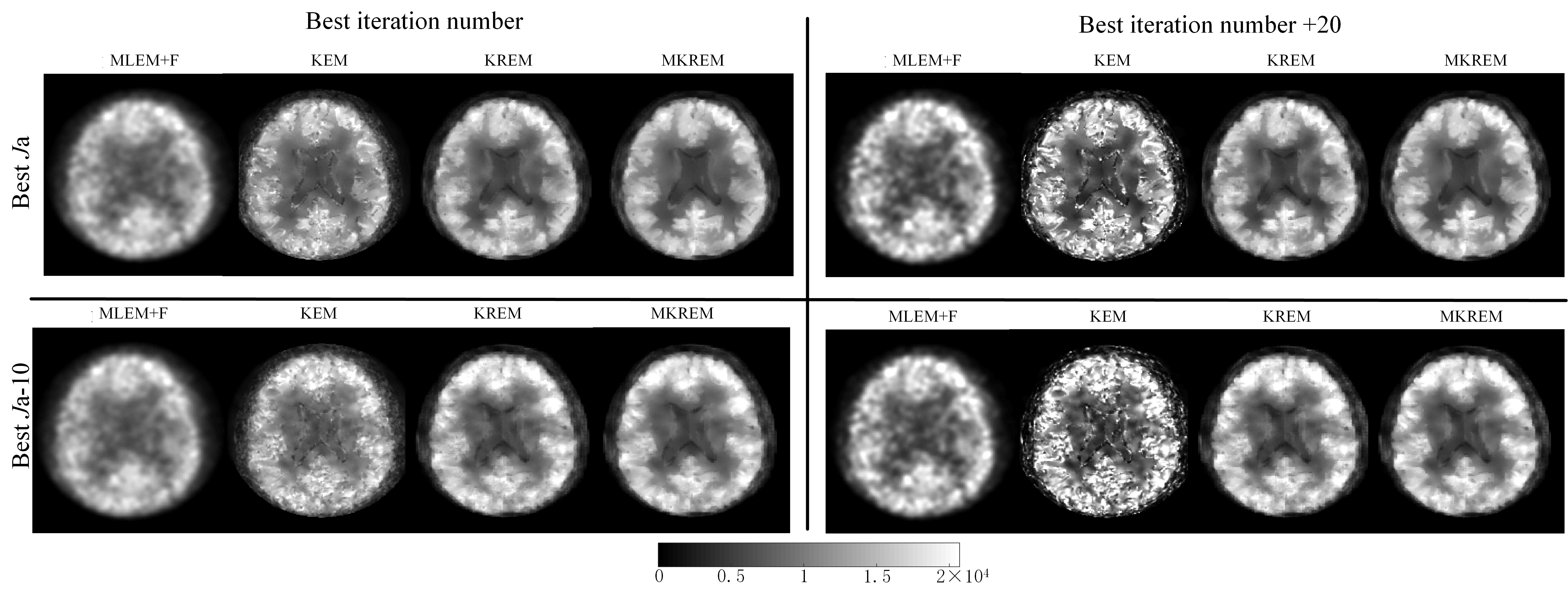
Based on the parameters from simulation studies, the parameters of all four methods were individually fine-tuned to achieve their respective best visual performance. The images thus reconstructed are shown in the upper-left panes of Fig. 8 and Fig. 9. Compared with MLEM+F and KEM, KREM and MKREM images have better visual effect, with clearer edges and details, and MKREM also further outperforms KREM.
To validate the robustness of KREM and MKREM, we detuned the best iteration numbers and the best neighborhood sizes (excluding MLEM+F) of all four methods. The reconstructed images of the four methods under three different scenarios of the detuned parameters are shown in the upper-right, lower-left and lower-right panes of Fig. 8 and Fig. 9. It can be seen that the MLEM+F and KEM images have changed quite noticeably under the detuned parameters, becoming noisy and showing image artifacts. In contrast, the changes in KREM and MKREM images, especially in MKREM images, are barely noticeable. These demonstrate the superior robustness of KREM and MKREM and the sensitivity of MLEM+F KEM to their tuning parameters in real life applications.
The above tests were conducted using Matlab 2016b on a PC with an Intel Core i7 3.60GHz CPU. The computation time with the uncompiled Matlab code was 34 s for KREM and 128 s for MKREM over 40 iterations.
5 Discussions
The results of simulation studies and in vivo data tests clearly show that KREM and MKREM outperform MLEM+F and KEM, achieving lower AMSE, faster convergence speed, simultaneously lower bias and variance, lower sensitivity to the neighborhood size , and high robustness to the iteration number. Moreover, all these advantages are more pronounced for MKREM.
The superior reconstruction performance of KREM and MKREM over MLEM+F and KEM can be attributed to the anatomical information of training images embedded in and enforced by the kernel space dictionary and the graph Laplacian quadratic in the two regularizers of KREM and MKREM. The KREM and MKREM’s much faster convergence speed and high robustness to the iteration number can be attributed to their two regularizers. And the better performance of MKREM over KREM can be attributed to its distinct multi-kernel matrices used in the dictionary learning, Laplacian matrix construction and MKREM algorithm (25).
For the low count case in Fig. 7(a), the larger the , the lower the MSE. This is because denoising is the key to reduce AMMSE in low count case. With larger , the algorithms use more neighboring pixels to reconstruct a pixel, which smooths out the noise and hence decreases AMMSE. While for the high count case in Fig. 7(b), the algorithms achieve minimum AMMSE at a smaller , eg for MKREM, a further increase of will increase AMMSE. This is because the key to reduce AMMSE in this case is not denoising but edges preserving. A larger could blur the details and edges and thereby increases AMMSE. Moreover, larger leads to denser kernel matrix and increases greatly computation cost. Whereas, is generally needed in dictionary learning for the kernel to capture the image details in high resolution image priors, eg in our simulation studies and in vivo data tests.
6 Conclusion
This paper has presented a novel solution to the problems of the recently emerged kernelized MLEM methods in potentially large reconstruction error and high sensitivity to iteration number. The solution has provided a general framework for developing the regularized kernelized MLEM with multiple kernel matrices and multiple kernel space regularizers for different PET imaging applications. The presented general class of multi-kernel matrices and two specific kernel space regularizers have resulted in the KREM and MKREM algorithms. Extensive test and comparison results have shown the superior performance of these new algorithms and their advantages over the kernelized MLEM and other conventional iterative methods in PET image reconstruction.
The multiple kernel and multiple regularizer framework of the MKREM algorithm (14) has offered many possibilities for further performance improvements. For example, instead of the MR anatomical image priors, we can also use other prior data, alone or mixed with MRI data, to construct the multi-kernel matrices, kernel image dictionary and Laplacian matrix for (14). We have mixed both the spatial and temporary priors to construct these matrices and have obtained excellent results in dynamic PET imaging, with much improved spatial and temporal resolutions. Moreover, we may use the multiple kernel leaning approach developed in machine learning [31, 32] to learn more general kernel polynomials from prior data and hence obtain the optimal multi-kernel matrices for an application, instead of constructing them by careful selection of the kernels and their combinations manually. These results will be reported in future works.
References
- [1] M. N. Wernick and J. N. Aarsvold, “Emission tomography: the fundamentals of PET and SPECT,” Elsevier, 2004.
- [2] H. H. Barrett, D. W. Wilson, and B. M. Tsui, “Noise properties of the EM algorithm: I. Theory,” Physics in Medicine & Biology, no. 39, vol. 5, pp. 833-846, 1999.
- [3] E. Levitan and G. T. Herman, “A maximum a posteriori probability expectation maximization algorithm for image reconstruction in emission tomography,” IEEE Transactions on Medical Imaging, vol. 6, no. 3, pp. 185-192, 1987.
- [4] P. J. Green, “Bayesian reconstructions from emission tomography data using a modified EM algorithm,” IEEE Transactions on Medical Imaging, vol. 9, no. 1, pp. 84 - 93, 1990.
- [5] D. Lalush and B. Tsui, “Simulation evaluation of Gibbs prior distributions for use in maximum a posteriori SPECT reconstructions,” IEEE Transactions on Medical Imaging, no. 11, vol. 2, pp. 267-275, 1992.
- [6] G. Gindi, M. Lee, A. Rangarajan, and I. G. Zubal, “Bayesian reconstruction of functional images using anatomical information as priors,” IEEE Transactions on Medical Imaging, vol. 12, no. 4, pp. 670-680, 1993.
- [7] J. E. Bowsher, H. Yuan, and L. W. Hedlund, “Utilizing MRI information to estimate F18-FDG distributions in rat flank tumors,” IEEE Nuclear Science Symposium Conference Record, 2004, pp. 2488-2492.
- [8] M. J. Ehrhardt, “PET reconstruction with an anatomical MRI prior using parallel level sets,” IEEE Transactions on Medical Imaging, vol. 35, pp. 2189-2199, 2016.
- [9] K. Vunckx, A. Atre, K. Baete, and A. Reilhac, “Evaluation of three MRI-based anatomical priors for quantitative PET brain imaging,” IEEE Transactions on Medical Imaging, vol. 31, pp. 599-612, 2012.
- [10] J. Jiao, N. Burgos, D. Atkinson, B. Hutton, and S. Arridge, “Detail-preserving PET reconstruction with sparse image representation and anatomical priors,” Information Processing in Medical Imaging, vol. 24, pp. 540-550, 2014.
- [11] J. Tang, A. Rahmim, “Bayesian PET image reconstruction incorporating anato-functional joint entropy,” Physics in Medicine & Biology, no. 54, vol. 32, pp. 63-75, 2009.
- [12] B. Yang, L. Ying, and J. Tang, “Artificial neural network enhanced Bayesian PET image reconstruction,” IEEE Transactions on Medical Imaging, vol. 37, pp. 1297-1309, 2018.
- [13] J. Tang, Y. Wang, R. Yao, and L Ying, “Sparsity-based PET image reconstruction using MRI learned dictionaries,” International Symposium on Biomedical Imaging, Beijing, China, April, 2014, pp. 1087-1090.
- [14] V. P. Sudarshan, G. F. Egan, and Z. Chen, “Joint PET-MRI image reconstruction using a patch-based joint-dictionary prior,” Medical Image Analysis, vol. 62, pp. 1-24, 2020,
- [15] A. Mehranian, M. A. Belzunce, and C. Prieto, “Synergistic PET and SENSE MR image reconstruction using joint sparsity regularization,” IEEE Transactions on Medical Imaging, vol. 37, no. 1, pp. 20-34, 2017.
- [16] F. Knoll, M. Holler, and T. Koesters, “Joint MR-PET reconstruction using a multi-channel image regularizer,” IEEE Transactions on Medical Imaging, vol. 36, no. 1, pp. 1-16, 2016.
- [17] W. Hutchcroft, G. B. Wang, and K. T. Chen, “Anatomically-aided PET reconstruction using the kernel method,” Physics in Medicine & Biology, vol. 61, no. 18, pp. 66-68, 2016.
- [18] G. B. Wang, J. Qi, “PET image reconstruction using kernel method,” IEEE Transactions on Medical Imaging, no. 34, vol. 1, pp. 61-71, 2015.
- [19] D. Deidda, N. Karakatsanis, and P. Robson, “Hybrid PET-MR list-mode kernelized expectation maximization reconstruction,” Inverse Problems, no. 35, vol. 4, pp. 1-24, 2019.
- [20] G. B. Wang, “High temporal-resolution dynamic PET image reconstruction using a new spatiotemporal kernel,” IEEE Transactions on Medical Imaging, no. 38, vol. 3, pp. 664-674, 2019
- [21] J. Bland et al. “MR-guided kernel EM reconstruction for reduced dose PET imaging,” IEEE Transactions on Radiation and Plasma Medical Sciences, no. 2, vol. 3, pp. 235-243, 2018.
- [22] P. Novosad and A. J. Reader, “MR-guided dynamic PET reconstruction with the kernel method and spectral temporal basis functions,” Physics in Medicine & Biology, no. 61, vol. 12, pp. 4624-4645, 2016.
- [23] K. Gong, J. Cheng-Liao, G. B. Wang, K. T. Chen, C. Catana, and J. Qi, “Direct Patlak reconstruction from dynamic PET data using kernel method with MRI information based on structural similarity,” IEEE Transactions on Medical Imaging, no. 37, vol. 4, pp. 955-965, 2018.
- [24] J. Bland, M. Belzunce, S. Ellis, C. McGinnity, and A. Hammers, “Spatially-compact MR-guided kernel EM for PET image reconstruction,” IEEE Transactions on Radiation and Plasma Medical Sciences, vol. 2, no. 5, pp. 470-482, 2018.
- [25] S. Ellis and A. Reader, “Kernelised EM image reconstruction for dual-dataset PET studies,” IEEE Nuclear Science Symposium, Medical Imaging Conference and Room-Temperature Semiconductor Detector Workshop, Strasburg, France, pp. 1-3, 2016.
- [26] R. Baikejiang, Y. Zhao, B. Z. Fite, K. W. Ferrara, and C. Q. Li, “Anatomical image guided fluorescence molecular tomography reconstruction using kernel method,” Journal of Biomedical Optics, no. 22, vol. 5, pp. 055-067, 2017.
- [27] B. Spencer and G. Wang, “Statistical image reconstruction for shortened dynamic PET using a dual kernel method,” in Proceedings of NSS/MIC, Atlanta, GA, USA, September, 2017.
- [28] A.J. Smola and R. Kondor, “Kernels and Regularization on Graphs,” Learning Theory and Kernel Machines, 2003.
- [29] C. I. Oliver, “Markov processes for stochastic modeling,” 2nd Ed, Elsevier, 2013.
- [30] J. Taylor and N. Cristianini, “Kernel methods for pattern analysis,” Cambridge University Press, 2004.
- [31] M. Gonen and E. Alpaydin, “Multiple kernel learning algorithms,” Journal of Machine Learning Research, vol. 12, pp. 2211-2268, 2011.
- [32] C. Cortes, M. Mohri, and A. Rostamizadeh, “Learning non-linear combinations of kernels,” Proceedings of the 22nd International Conference on Neural Information Processing Systems, 2009, pp. 396-404.
- [33] M. Elad, “Sparse and redundant representations from theory to Aapplications in signal and image processing,” Springer, 2010.
- [34] D. I. Shuman, S. K. Narang, P. Frossard, A. Ortega, and P. Vandergheynst, “The emerging field of signal processing on graphs: extending high-dimensional data analysis to networks and other irregular domains,” in IEEE Signal Processing Magazine, vol. 30, no. 3, pp. 83-98, 2013.
- [35] D. van Dijk et al., “Recovering gene interactions from single-cell data using data diffusion,”Cell, vol. 174, no. 3, pp. 716-729, 2018.
- [36] C.A. Cocosco, V. Kollokian, R.K.-S. Kwan, and A.C. Evans, “BrainWeb: Online interface to a 3D MRI simulated brain database,” Proceedings of 3rd International Conference on Functional Mapping of the Human Brain. Copenhagen, Denmark, May, 1997.
- [37] D. L. Collins et al. “Design and construction of a realistic digital brain phantom,” IEEE Transactions on Medical Imaging, vol. 17, no. 3, pp. 463-468, 1998.
- [38] S. D. Jamadar, P. G. Ward, E. X. Liang, E. R. Orchard, Z. Chen, and G. F Egan, “Metabolic and haemodynamic resting-state connectivity of the human brain: a high-temporal resolution simultaneous BOLD-fMRI and FDG-fPET multimodality study,” Neuroscience, https://doi.org/10.1101/2020.05.01.071662”