hailong2019@iscas.ac.cn (H. Sheng), chao_yang@pku.edu.cn (C. Yang)
PFNN-2: A Domain Decomposed Penalty-Free Neural Network Method for Solving Partial Differential Equations
Abstract
A new penalty-free neural network method, PFNN-2, is presented for solving partial differential equations, which is a subsequent improvement of our previously proposed PFNN method [1]. PFNN-2 inherits all advantages of PFNN in handling the smoothness constraints and essential boundary conditions of self-adjoint problems with complex geometries, and extends the application to a broader range of non-self-adjoint time-dependent differential equations. In addition, PFNN-2 introduces an overlapping domain decomposition strategy to substantially improve the training efficiency without sacrificing accuracy. Experiments results on a series of partial differential equations are reported, which demonstrate that PFNN-2 can outperform state-of-the-art neural network methods in various aspects such as numerical accuracy, convergence speed, and parallel scalability.
keywords:
neural network, penalty-free method, domain decomposition, initial-boundary value problem, partial differential equation.65M55, 68T99, 76R99
1 Introduction
In recent years, neural network methods are becoming an attractive alternative for solving partial differential equations (PDEs) arising from applications such as fluid dynamics [2, 3, 4], quantum mechanics [5, 6, 7], molecular dynamics [8], material sciences [9] and geophysics [10, 11]. In contrast to most traditional numerical approaches, methods based on neural networks are naturally meshfree and intrinsically nonlinear therefore can be applied without going through the cumbersome step of mesh generation and could be more potentially applicable to complicated nonlinear problems. These advantages have enabled neural network methods to draw increasingly more attention with both early studies using shallow neural networks [12, 13, 14, 15, 16, 17, 18] and recent works with the advent of deep learning technology [19, 20, 21, 5, 22, 23, 24, 25].
Despite of the tremendous efforts to improve the performance of neural network methods for solving PDEs, there are still issues that require further study. The first issue is related to the accuracy of neural network methods. It is still not fully understood how well a neural network can approximate the solution of a PDE in either theory or practice. Recent investigations were carried out to reveal some preliminary approximation properties of neural networks for simplified problems [26, 27, 28, 29], or to improve the accuracy of neural network methods from various aspects such as by introducing weak form loss functions to relax the smoothness constraints [21, 30, 31, 32, 33, 34], by modifying the solution structure to automatically satisfy the initial-boundary conditions [15, 17, 18, 35, 36], by revising the network structure to enhance its representative capability [37, 38, 39, 40], and by introducing advanced sampling strategies to reduce the statistical error [41, 42]. These improvements so far are usually effective in respective situations, but are not general enough to adapt with different types of PDEs defined on complex geometries.
Another difficulty for solving PDEs with neural network methods is related to the efficiency. It is widely known that training a neural network is usually much more costly than solving a linear system resulted from a traditional discretization of the PDE [43, 44, 45]. To improve the efficiency, it is natural and has been extensively considered [4, 46] to utilize distributed training techniques [47, 48] based on data or model parallelism, by which the training task is split into a number of small sub-tasks according to the partitioned datasets or model parameters so that multiple processors can be exploited. Although this distributed training is general and successful in handling many machine learning tasks [49, 50, 51, 52], it is not the most effective choice for solving PDEs because no specific knowledge of the original problem is adopted throughout the training process.
Inspired by the idea of classical domain decomposition methods [53], it was proposed to introduce domain decomposition strategies into neural network based PDE solvers [54, 55, 56, 57, 58, 59, 60, 61, 62] by dividing the learning task into training a series of sub-networks related to solutions on sub-domains. This tends to be more natural than the plain distributed training approaches because by introducing domain decomposition the training of each sub-network only requires a small part of dataset related to the corresponding sub-domain, therefore can significantly decrease the computational cost. However, these methods may still suffer from issues related to low convergence speed and poor parallel scalability due in large part to the straightforward treatment of artificial sub-domain boundaries.
In this paper, we present PFNN-2, a new penalty-free neural network method that is a subsequent improvement of our previously proposed PFNN method [1]. Inheriting all advantages of PFNN in handling the smoothness constraints and essential boundary conditions of self-adjoint PDEs, PFNN-2 extends the application to a broader range of non-self-adjoint time-dependent problems and introduces a domain decomposition strategy to improve the training efficiency. In particular, PFNN-2 employs a Galerkin variational principle to transform the non-self-adjoint time-dependent equation into a weak form, and adopts compactly supported test functions that are convenient to build on complex geometries. To further reduce the difficulty of the training process and improve the accuracy, PFNN-2 separates the penalty terms related to the initial-boundary constraints from the loss function, with a dedicated neural network learning the initial and essential boundary conditions, and the true solution on the rest of the domain approximated by another network that is totally disentangled from the former one. On top of the above, PFNN-2 introduces an overlapping domain decomposition strategy to speedup multi-processor training without sacrificing accuracy, thanks to the penalty-free treatment of initial-boundary conditions of the decomposed sub-problems and the weak form loss function with reduced smoothness requirement. We carry out a series of numerical experiments to demonstrate that PFNN-2 is advantageous over existing state-of-the-art algorithms in terms of both numerical accuracy and computational efficiency.
The remainder of the paper is organized as follows. In Section 2 we present the basic algorithms employed in PFNN-2 to handle the smoothness constraints and initial-boundary conditions. Following that the domain decomposition strategy adopted by PFNN-2 for parallel computing is introduced in Section 3. We then discuss and compare PFNN-2 with several related state-of-the-art neural network methods in Section 4. Numerical experiment results on a series of linear and nonlinear, time-independent and time-dependent, initial-boundary value problems on simple and complex geometries are reported in Section 5. The paper is concluded in Section 6.
2 The PFNN-2 method
For the ease of discussion, we first consider the case of a single sub-domain () on which we try to solve the following initial-boundary value problem:
| (1) |
where , and are dependent on the solution as well as the spatial and temporal coordinates and , and is the outward unit normal. Both Dirichlet and Neumann boundary conditions are considered, with the corresponding boundaries and .
To reduce the smoothness requirement, we introduce the following weak form
| (2) |
with the solution belonging to a trial (hypothesis) space and satisfying initial-boundary conditions
where is a certain test space, in which any function satisfies on .
In PFNN-2, the approximate solution of problem (2) is found within the hypothesis space that is formed by neural networks. Unlike most of the existing methods [19, 20, 21, 30, 31, 32, 34] that merely apply a single network to construct , PFNN-2 adopts two neural networks, with one network learning the solution with the initial condition and essential boundary condition more accurately and swiftly, and another network approximating the solution on the rest part of the domain, where , donate the sets of weights and biases forming the two networks, respectively. To eliminate the influence of on the initial condition and essential boundary condition, a length factor function is introduced to impose appropriate restriction, which satisfies
| (3) |
With the help of the length factor function, any function in the hypothesis space is constructed as follows:
| (4) |
where .
The length factor function is established by utilizing spline functions, which are more flexible to adapt to various complicated geometries than the analytical functions proposed in previous works [15, 35, 36]. To be specific, we divide the essential boundary into several segments , . For each segment , select another segment of the boundary as its companion (note that should not be adjacent to ). Then, for each , a spline function is built, which satisfies
| (5) |
The specific details to construct can be found in our previous work of PFNN [1]. Utilizing all the functions, the length factor function , which is dependent on both space and time, is established by:
| (6) |
where is adopted for adjusting the shape of . In order to avoid that the value of drops dramatically with the growth of , we suggest that .
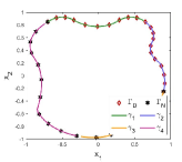
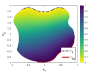
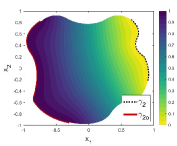
Figure 1 is an example to demonstrate how to construct the function , in which the essential boundary is divided into two parts, and . Correspondingly, another two segments, and , are taken from the Neumann boundary as the companions and , respectively. Then two spline functions and satisfying (5) can be built according to the method in PFNN [1] and the length factor function is established according to (6).
To improve the flexibility to complex geometries and reduce the cost to evaluation residual (2), rather than the commonly utilized orthogonal polynomials [32, 33], a set of compactly supported test functions
| (7) |
are employed to span the test space , where and are the center and radius of the support of , respectively, and and are the th element of and , respectively. The center is sampled on while the radius is small to ensure that the residual can be just evaluated on a tiny region instead of the whole domain. To achieve this, the radius is set to:
| (8) |
where is the minimum distance from to so that on , and is the upper bound of , which is defined as
Such configuration keeps and guarantees that the supports of all the test functions could cover most part of the computing domain.
Since the two neural networks and are decoupled by the length factor function , they can be trained separately. First, is trained to learn the initial and essential boundary condition via minimizing the loss function
| (9) |
where represents a set of points sampled on . Then, let be the obtained network after minimizing (9) and . An approximate solution of problem (2) can be obtained by minimizing as follows:
| (10) |
where
| (11) |
is the estimate of the residual of the governing equation (2), donates the size of . Eq. (10) is taken as the loss function for training . It can be seen that neither of the loss functions (9) and (10) involves any penalty term, therefore is easier to minimize than those with penalty terms frequently found in various neural network methods for solving partial differential equations. Besides, the training of each network only needs data samples on part of the computing domain, which has less computational cost than training a single network with data samples from the whole domain.
3 Domain decomposition for PFNN-2
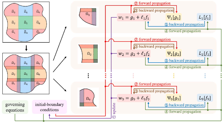
To enable parallel computing capability in PFNN-2, we first partition the computing domain into a group of non-overlapping sub-domains , and then extend each sub-domain to obtain a series of overlapping sub-domains , where is the number of sub-domains. Figure 2 shows an example of the overlapping domain decomposition partition for the case of . Starting with a suitable initial guess , problem (1) can be solved by constructing a solution sequence that converges to the true solution, where represents the count of iteration. And the approximate solution for each iteration is formed by solving a series of sub-domain problems concurrently on parallel computers. In particular, at the -th iteration the sub-domain problem defined on is
| (12) |
where , , and . After solving the sub-domain problems for iteration , the approximate solution defined on the whole domain is composed as .
To construct the solution sequence, instead of solving the sub-domain problem (12) directly, PFNN-2 finds an approximate solution to the corresponding sub-domain problem in the weak form
| (13) |
where belongs to a hypothesis space and satisfies the initial-boundary conditions
and is a certain test space.
Since the weak form (13) is similar to (2), we can utilize the method presented in the previous section to establish the hypothesis space and test space , for all . Specifically on sub-domain , is spanned by a set of compactly supported functions (), and any function is constructed according to
| (14) |
where and are two sub-networks that play roles similar to and , and is a length factor function that decouples the two sub-networks. Note that here and hereafter, we drop the subscripts representing the learnable parameters for brevity.
Starting from a proper initial state , each local approximate solution is updated by a dedicated processor to produce a sequence converging to the corresponding local true solution, where and are the initial states of sub-networks and , is the count of iteration. In the -th iteration, is acquired by solving the corresponding sub-problem (13). And following that, all the are merged together to form the approximate solution on the whole domain according to . To illustrate the solving process accurately and intuitively, Algorithm 1 and Figure 2 are provided, which show that each iteration is comprised of two stages:
-
•
Online stage (line 4-13 of Algorithm 1): As demonstrated in step ① of Figure 2, each processor conducts communication to the immediate neighbors to acquire the current interior boundary condition, where satisfies , on .
-
•
Offline stage (line 15-23 of Algorithm 1): First, as shown in steps ②-③ of Figure 2, each sub-network is trained on the corresponding processor to learn the local solution by minimizing the loss function
(15) Let be the acquired sub-network after minimizing (15) and . Then, as shown in steps ④-⑤ of Figure 2, each sub-network is trained on the corresponding processor to approximate the local solution on the remainder of the sub-domain via minimizing
(16) Afterwards, the obtained sub-network is utilized to form the local approximate solution . And finally, the approximate solution on the whole domain is composed as .
4 Discussion and comparison with other related methods
In this section, we review several state-of-the-art neural network methods for solving PDEs and compare them with PFNN-2. For simplicity we consider a model boundary value problem
| (17) |
The most commonly applied neural network algorithms are based on the idea of least squares; examples can be found in e.g., Refs. [14, 15, 17, 19, 2, 63]. In a least-squares based method, an approximate solution of (17) is found by minimizing the loss function in the least-squares form as follows:
| (18) |
where is a penalty coefficient. Despite of being straightforward to implement, this approach may encounter issues of low convergence speed and poor accuracy, primarily because the complicated loss function usually requires simultaneously approximating the high-order derivatives of the solution and the additional initial and boundary conditions, thus imposing extreme difficulty for optimization. In addition, the training of the highly nonlinear neural network may also demand large computational cost and lead to low computational efficiency.
4.1 Accuracy improvement
Several neural network methods were proposed to enhance the accuracy by lowering the smoothness requirement so that high-order differential operators involved in the loss function are eliminated. These methods can be roughly classified into two categories, involving weak forms based on the Ritz and Galerkin variational principles, respectively.
In approaches based on the Ritz variational principle such as the ones presented in Refs. [21, 30, 64, 65], the original problem in the strong form (17) is transformed to an energy minimization problem
| (19) |
where is a certain hypothesis space built by neural networks. In this way, the high-order derivatives are avoided in the loss function. However, the scope of applications of these methods is usually relatively narrow, confined to self-adjoint elliptic problems.
In methods based on the Galerkin variational principle, an approximate solution is found within a hypothesis space satisfying
| (20) |
where is a certain test function space. Although having a wider applications than Ritz-type approaches, existing Galerkin-based neural network methods are usually in lack of flexibility and efficiency. For example, orthogonal polynomials can be employed as the test functions [32, 33], but the methods are only applicable to simple geometries for which orthogonal polynomials are known. It is also possible to take compactly supported piecewise linear functions to construct the test space with low cost [31], which however requires a grid to arrange the locations of the test functions and is again hard to adapt to complex geometries. In some recent works [34, 66], an adversarial network was introduced to evaluate the maximum weighted loss in an adaptive manner, but the method is often hard to converge because of the difficulty in balancing the efforts devoted to training the generative network for the approximate solution and the adversarial network for the test function.
Apart from relaxing the smoothness constraints, there are another series of neural network methods that aim to improve the accuracy by removing the boundary constraints [15, 17, 18, 35, 36]. The basic idea is to establish the approximate solution in the form of
| (21) |
where is manufactured to satisfy boundary conditions, is a network for learning the true solution within the domain, and is introduced to eliminate the influence of the network on the boundary. The main disadvantage of these methods is lacking a universal and flexible strategy to build the functions and . For handling a specific problem on a particular domain, most of the works [15, 35, 36] rely on a dedicated function in the analytical form, which usually cannot be applied to any other case. Although some efforts have been made [17, 18] by introducing spline functions so that the method can be applied to a broader range of computing domains, the flexibility is still very limited.
The proposed PFNN-2 method integrates the advantages of all the aforementioned methods. With the introduction of the weak form loss function, the burdensome task of approximating the high-order derivatives are avoided. By separating the task of learning initial and essential boundary conditions from other training tasks, the constraints are dealt with in a more effective manner, and the subsequent training process is eased because the penalty terms in the corresponding loss function are eliminated. The structures of the approximate solution comprised of neural networks and spline functions as well as the compactly supported test functions have a high flexibility, which can extend the applicability of the method to a wide range of PDEs.
4.2 Domain decomposition
In a classical numerical method for solving PDEs, the idea of domain decomposition can be introduced by transforming the solution of the original problem into solving a number of simpler sub-problems defined on a series of sub-domains (). Starting from an appropriate initial guess , a solution sequence () is built to approach to the true solution of the original problem. In particular, for problem (17), at the -th iteration, is formed by composing a set of local approximate solutions , which are acquired by solving sub-domain problems
| (22) |
in parallel, where and are certain differential operators, whose forms depend on the specific method employed.
Previously proposed domain decomposition methods for neural network based solution of PDEs can be categorized into two major classes: overlapping and non-overlapping methods. Figure 2 has already illustrated the difference between the two. Among existing works, DeepDDM [54] and D3M [56] are overlapping methods, and cPINNs [57, 59] and XPINNs [58, 59] are non-overlapping ones. Depending on the partition strategies adopted, as well as other characteristics, the differential operators and in these methods are in various forms, as briefly listed below.
-
•
DeepDDM:
(23) -
•
D3M:
(24) where is an additional variable to approximate the gradient of the solution .
-
•
cPINNs:
(25) -
•
XPINNs:
(26)
In general, the aforementioned methods solve sub-problems (22) by introducing sub-networks to approximate the local solutions on , respectively. After initialized properly to form the initial states , the sub-networks are trained in parallel to generate solution sequences converging to local true solutions, where is the iteration count, and is acquired by minimizing the loss function
| (27) |
Correspondingly, a solution sequence defined on the whole domain is formed by combining all the updated sub-networks together.
In contrast to the existing domain decomposition based neural network methods that utilize loss functions in strong form (27), PFNN-2 employs weak form loss functions to avoid the explicit computation of high order derivatives of the approximate solution, and therefore has a higher computing efficiency. In addition to that, thanks to the penalty-free property, PFNN-2 is able to reduce the difficulty of the network training process and improve the sustained accuracy. As demonstrated in later numerical experiments, all these advantages make PFNN-2 a more suitable candidate for the case of multiple sub-domains, especially when the number of sub-domains is large.
5 Numerical Experiments
In this section, we carry out a series of numerical experiments to investigate the performance of the proposed PFNN-2 method, and compare it with several existing state-of-the-art approaches. Four test cases are utilized to examine the accuracy and efficiency of different numerical methods. In all tests involving neural networks, the ResNet model [67] with sinusoid activation function is utilized for constructing the network, in which each ResNet block is comprised of two fully connected layers and a residual connection. Note that PFNN-2 utilizes two neural networks instead of one. To make fair comparison between various methods, we try to adjust the number of ResNet blocks and the width of hidden layers so that the total degree of freedoms (i.e., parameters including weights and biases for neural network methods, and unknowns for traditional methods) is kept to a similar level. The L-BFGS optimizer [68] is applied for training the neural networks. All the experiments are conducted on a computer equipped with Intel Xeon Gold 6130 CPUs. And all calculations are done with 32-bit floating point computations. The relative -error is taken to measure the accuracy of the approximate solutions. All the results obtained with neural network methods are reported based on ten times of independent experiments.
5.1 Anisotropic convection-diffusion equation on an L-shaped domain
The first test case is an anisotropic convection-diffusion equation
| (28) |
defined on an L-shaped domain , where
We set the solution to be , where is the polar coordinate, and let be derived accordingly. We apply Neumann boundary condition on and Dirichlet boundary condition on the rest of the boundary . The main difficulty of solving this problem is the singularity near the inner corner of the L-shaped domain.
We run the test with only one processor to examine the performance of various methods without domain decomposition. It should be noted that not all neural network methods based on variational principles can be applied to this problem. In particular, some methods such as Deep Ritz [21] and Deep Nitsche [30] is only suitable for self-adjoint problems, some such as VPINNs [32] and hp-VPINNs [33] require orthogonal polynomials to form the test spaces, which are hard to build on irregular domains. Therefore, in this test, we only examine methods including the traditional linear finite element method, the least-squares neural network method, a variational neural network method called VarNet [31] (which takes compactly supported piecewise linear functions as test functions) and PFNN-2. For PFNN-2, we sample 1200 points in and 80 points on as the centers to form the test functions according to the strategy specified in section 2, and sample 160 points on . For the other neural network methods, the training sets with similar size are adopted. The maximum number of iterations for training neural networks is set to 6000 epochs.
| Method | finite element | least-squares | VarNet | PFNN-2 |
|---|---|---|---|---|
| Network | - | 3 blocks (width:15) | 3 blocks (width:15) | 23 blocks (width:10) |
| DOFs | 1242 | 1261 | 1261 | 1182 |
| Relative [1.5mm] error | 2.32e-03 | 1.38e-026.12e-03 | 1.56e-023.43e-03 | 9.18e-043.37e-04 |
| 6.64e-033.02e-03 | 6.71e-031.38e-03 | |||
| 1.06e-024.93e-03 | 6.82e-031.98e-03 |
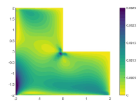
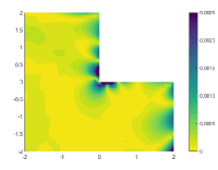
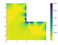
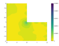
The relative errors of the approximate solutions obtained by the tested algorithms are reported in Table 1, in which the influence of penalty factor for the least-squares neural network method and VarNet is also investigated. It can be seen from the table that the two penalty-based methods is inferior to the classical finite element method in terms of accuracy for this test case, and their performance is seriously affected by the change of penalty factors. In contrast, PFNN-2 is free of any penalty term and is not subject to such influence, thus can outperform all the methods in terms of sustained accuracy. Further, we draw the distribution of the solution errors of the tested algorithms in Figure 3, from which we observe that there are significant errors occurring near the corner of the L-shaped domain when the finite element method and the penalty-based neural network approaches are used, indicating the inefficient treatment of corner singularity. In addition, the two penalty-based neural network methods also have serious errors near the essential boundary. PFNN-2, on the other hand, is free of such singularity and boundary effects, and can sustain the most accurate result among the tested methods, with the error uniformly distributed both within the domain and on the boundary.
5.2 Allen-Cahn equation on a periodic domain
The next test case is the well-known Allen-Cahn equation [69] for phase field simulation:
| (29) |
defined on a periodic domain . We set the width of the transition layer to be and set the initial condition to be
For this time-dependent problem, we conduct the simulation from to .
The true solution of the above problem has some sharp gradients on the transition layer. For dealing with the problem, domain decomposition based methods tend to be effective, since each network only need to learn one part of the solution. To examine the effectiveness of the domain decomposition strategies of various neural network methods including cPINNs, XPINNs, DeepDDM, D3M and PFNN-2, four groups of experiments are conducted, in which the computational domain is decomposed into 11, 33, 55 and 77 sub-domains, respectively. Configurations of the network structures for the various tested methods are listed in Table 2, where we try to maintain a similar amount of learnable parameters for each group of the test. We sample 16000 points on the whole computational domain to form the test function sets. The numbers of outer and inner iterations are set to be 150 and 40, respectively, resulting a total of 6000 iterations. A numerical solution obtained by the Fourier spectral method with 1024 modes and second-order explicit Runge-Kutta temporal integrator with time step is taken as the ground truth for evaluating the solution error. Different penalty coefficients including 1, 10, 100 and 1000 are examined for penalty-based methods and the value with the optimal performance is picked out for further analysis.
| cPINNs/XPINNs/DeepDDM | D3M | PFNN-2 | |
|---|---|---|---|
| 1 | 14 blocks (width:32) | 14 blocks (width:32) | 124 blocks (width:22) |
| 7553 DOFs | 7619 DOFs | 7306 DOFs | |
| 9 | 92 blocks (width:15) | 92 blocks (width:15) | 922 blocks (width:10) |
| 7164 DOFs | 7452 DOFs | 6858 DOFs | |
| 25 | 251 blocks (width:14) | 251 blocks (width:14) | 2521 blocks (width:9) |
| 7025 DOFs | 7775 DOFs | 6800 DOFs | |
| 49 | 491 blocks (width:10) | 491 blocks (width:10) | 4921 blocks (width:6) |
| 7889 DOFs | 8967 DOFs | 7154 DOFs |
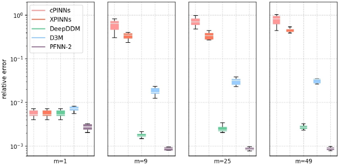
Figure 4 provides an intuitive display of the numerical accuracy of different tested methods, in which box-plots are drawn to describe the five-number summary including the minimum observation, first quartile, middle value, third quartile, and maximum observation for each set of tests. It can be seen that not all domain decomposition strategies can improve the accuracy. As the number of sub-domains increases, the achievable accuracy of most of the existing domain decomposition based neural network methods except DeepDDM gets worse, which reveals their drawbacks in handling multiple sub-problems with constraints. Although DeepDDM can maintain a relatively satisfying accuracy, PFNN-2 has a more preferable performance, primarily due to its capability of dealing with smoothness constraints and boundary conditions.
5.3 Nonlinear anisotropic convection-diffusion equation on an irregular domain
In this test case, we consider a nonlinear anisotropic convection-diffusion equation
| (30) |
defined on an irregular domain with the shape of the Antarctica, as demonstrated in Table 3. We set the exact solution to be that satisfies the Dirichlet boundary condition, and set the coefficients to be
and is derived according to (30).
| 1 | 14 | 26 | 42 | |
| Network (cPINNs/ | 14 blocks (width:30) | 142 blocks (width:11) | 261 blocks (width:13) | 421 blocks (width:10) |
| DeepDDM) | 6661 DOFs | 6328 DOFs | 6448 DOFs | 6762 DOFs |
| Network (PFNN-2) | 124 blocks (width: | 1422 blocks (width: | 2621 blocks (width: | 4221 blocks (width: |
| 20) 6082 DOFs | 7) 5712 DOFs | 8) 5876 DOFs | 6) 6132 DOFs | |
| Decomposition of the domain | ![[Uncaptioned image]](https://cdn.awesomepapers.org/papers/0c2d12b4-ee14-4e29-bae1-6a814e22dd35/x11.png) |
![[Uncaptioned image]](https://cdn.awesomepapers.org/papers/0c2d12b4-ee14-4e29-bae1-6a814e22dd35/x12.png) |
![[Uncaptioned image]](https://cdn.awesomepapers.org/papers/0c2d12b4-ee14-4e29-bae1-6a814e22dd35/x13.png) |
![[Uncaptioned image]](https://cdn.awesomepapers.org/papers/0c2d12b4-ee14-4e29-bae1-6a814e22dd35/x14.png) |
To investigate the effectiveness of domain decomposition strategies of different neural network methods, we examine the performance of PFNN-2 and compare it with cPINNs and DeepDDM, which are selected as representative non-overlapping and overlapping domain decomposition neural network methods, respectively. We conduct four groups of experiments, in which the computational domain is decomposed into 1, 14, 26 and 42 sub-domains, respectively. In each group of experiments, we set network structure of each method with similar amount of undecided parameters, as illustrated in Table 3. A total of 6000 points are sampled on the whole computational domain to form the test function set. Other experiment configurations are the same to the previous experiment.
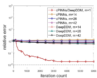
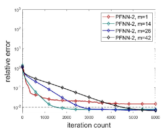
Figure 5 demonstrates the error evolution histories of various methods. It can be seen from the figure that it is hard for cPINNs and DeepDDM to converge to the true solution in the cases that multiple sub-domains are employed, which exposes their defects in tackling problem with strong nonlinearity. By comparison, thanks to the avoidance of penalty terms, as well as the reduction of the smoothness constraints and the flexble treatment of the complex geometry, PFNN-2 is more suitable for solving this problem and can achieve more accurate and stable results.
5.4 Viscous Burgers equation on a 3D cube
The last test case is a nonlinear equation system – the viscous Burgers equation
| (31) |
defined on domain with Dirichlet boundary condition defined on and Neumann boundary condition defined on , where the Reynolds number is . We set the true solution to be
and conduct the simulation from to .
In this test case, we examine both accuracy and efficiency of various methods including cPINNs, DeepDDM and PFNN-2. Firstly, the weak scaling efficiency of the tested methods is investigated. We conduct four sets of experiments, in which the computational domain is decomposed into 1, , and sub-domains, respectively. We keep the scale of task assigned to each processor similar. Specifically, we sample 5120 points on each sub-domain respectively to form the test function set, and adopt networks with similar scale to approximate local solution on each sub-domain, as illustrated in Table 4. Other experiment configurations are the same to the previous experiment. The accuracy of various method is reported in Table 4. Not surprisingly, the accuracy of all the methods is improved with the increase of the number of sub-domains, since the representative capability of approximate solution also grows stronger. In particular, PFNN-2 acquires the most accurate approximate solutions in all the test sets. Moveover, Figure 6 demonstrates the runtime for 400 iterations, which indicates that all the tested algorithms can maintain a relatively stable efficiency. In all the experiment groups, PFNN-2 always achieves the highest efficiency.
| Method | Network structure | DOFs | Errors () | Errors () | Errors () |
|---|---|---|---|---|---|
| cPINNs | 12 blocks (width:15) | 1828 | 7.31e-022.57e-02 | 1.31e-013.64e-02 | 1.34e-014.08e-02 |
| 82 blocks (width:15) | 8828 | 3.09e-028.38e-03 | 4.54e-021.33e-02 | 5.39e-021.63e-02 | |
| 162 blocks (width:15) | 16828 | 2.64e-027.40e-03 | 3.92e-021.02e-02 | 4.58e-021.36e-02 | |
| 322 blocks (width:15) | 32828 | 2.33e-026.92e-03 | 3.31e-028.19e-03 | 3.72e-028.76e-03 | |
| DeepDDM | 12 blocks (width:15) | 1828 | 7.31e-022.57e-02 | 1.31e-013.64e-02 | 1.34e-014.08e-02 |
| 82 blocks (width:15) | 8828 | 3.38e-021.15e-02 | 5.55e-021.58e-02 | 6.45e-022.12e-02 | |
| 162 blocks (width:15) | 16828 | 2.46e-026.74e-03 | 3.68e-021.13e-02 | 4.74e-021.48e-02 | |
| 322 blocks (width:15) | 32828 | 1.64e-025.41e-03 | 2.38e-027.20e-03 | 2.95e-027.87e-03 | |
| PFNN-2 | 122 blocks (width:10) | 1806 | 5.06e-021.36e-02 | 8.02e-022.14e-02 | 7.67e-022.05e-02 |
| 822 blocks (width:10) | 8806 | 2.23e-024.94e-03 | 2.76e-025.46e-03 | 3.22e-026.44e-03 | |
| 1622 blocks (width:10) | 16806 | 9.54e-032.27e-03 | 1.43e-023.69e-03 | 1.51e-023.83e-03 | |
| 3222 blocks (width:10) | 32806 | 6.72e-031.80e-03 | 9.72e-032.58e-03 | 9.81e-032.28e-03 |

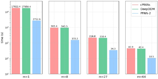
Next, the strong scaling efficiency of the tested approaches is examined. Four sets of experiments are carried out, in which the computational domain is split into , , and sub-domains, respectively. In this test, the overall scale of problem is kept similar in different test groups. To be specific, we sample 160,000 points on the whole computational domain to form the test function set, and keep the amounts of learnable parameters of different approaches in each group in a similar range, as shown in Table 5. Other experiment configurations are the same to the previous experiment. Table 5 also reports the solution errors of the various tested algorithms, which once more demonstrates the advantage of PFNN-2 with respect to the numerical accuracy. To further compare the performance in terms of computing time, we draw the runtime cost for 400 iterations in Figure 7, from which it can be seen that with the increase of the number of processors, the time-to-solution of all the methods is enhanced significantly. Among all the tested algorithms, PFNN-2 is always the most efficient.
| Method | Network structure | DOFs | Errors () | Errors () | Errors () |
|---|---|---|---|---|---|
| cPINNs | 15 blocks (width:72) | 47883 | 6.51e-022.63e-02 | 1.21e-013.77e-02 | 1.25e-013.85e-02 |
| 83 blocks (width:33) | 47016 | 3.36e-028.34e-03 | 4.78e-021.19e-02 | 5.39e-021.37e-02 | |
| 272 blocks (width:22) | 45819 | 2.89e-026.73e-03 | 3.77e-028.84e-03 | 4.05e-021.05e-02 | |
| 642 blocks (width:14) | 47680 | 2.70e-026.48e-03 | 4.03e-029.32e-03 | 3.92e-028.39e-03 | |
| DeepDDM | 15 blocks (width:72) | 47883 | 6.51e-022.63e-02 | 1.21e-013.77e-02 | 1.25e-013.85e-02 |
| 83 blocks (width:33) | 47016 | 3.81e-027.81e-03 | 4.76e-021.25e-02 | 6.13e-021.42e-02 | |
| 272 blocks (width:22) | 45819 | 1.60e-024.25e-03 | 2.31e-025.30e-03 | 2.58e-025.22e-03 | |
| 642 blocks (width:14) | 47680 | 1.21e-023.26e-03 | 1.75e-024.82e-03 | 1.72e-023.87e-03 | |
| PFNN-2 | 125 blocks (width:50) | 46706 | 4.59e-021.30e-02 | 6.73e-021.46e-02 | 5.92e-021.32e-02 |
| 823 blocks (width:23) | 47152 | 1.15e-023.26e-03 | 1.72e-024.56e-03 | 1.67e-024.30e-03 | |
| 2722 blocks (width:15) | 45522 | 6.49e-031.94e-03 | 9.37e-032.86e-03 | 9.22e-031.77e-03 | |
| 6421 blocks (width:15) | 46464 | 5.12e-031.63e-03 | 7.84e-032.03e-03 | 7.68e-031.96e-03 |
6 Conclusion
In this paper, a new penalty-free neural network method — PFNN-2 is presented for solving PDEs including non-self-adjoint time-dependent ones. PFNN-2 employs a Galerkin variational principle to convert the original equation into a weak form with low smoothness requirement, splits the problem with complex initial-boundary constraints into two simpler unconstrained ones, and adopts two neural networks to approximate the corresponding local solutions, which are then combined to form the approximate solution on the whole domain. A domain decomposition strategy is introduced in PFNN-2 to accelerate the training efficiency while maintaining the numerical accuracy. Experiment results demonstrate that PFNN-2 can surpass existing state-of-the-art in terms of accuracy, efficiency and scalability. Possible future explorations on PFNN-2 would involve the improvement on the network structure, the investigation on the error estimation, and the study on solving more challenging problems such as the ones with strong singularities.
Acknowledgments
This work was supported in part by National Natural Science Foundation of China (grant# 12131002).
References
- [1] H. Sheng, C. Yang, PFNN: A penalty-free neural network method for solving a class of second-order boundary-value problems on complex geometries, Journal of Computational Physics, 428 (2021) 110085.
- [2] M. Raissi, A. Yazdani, G. E. Karniadakis, Hidden fluid mechanics: Learning velocity and pressure fields from flow visualizations, Science, 367 (2020) 1026-1030.
- [3] X. Jin, S. Cai, H. Li, G. E. Karniadakis, NSFnets (Navier-Stokes flow nets): Physics-informed neural networks for the incompressible Navier-Stokes equations, Journal of Computational Physics, 426 (2021) 109951.
- [4] O. Hennigh, S. Narasimhan, M. A. Nabian, A. Subramaniam, K. Tangsali, Z. Fang, M. Rietmann, W. Byeon, S. Choudhry, NVIDIA SimNet: An AI-accelerated multi-physics simulation framework, in: International Conference on Computational Science, Springer, 2021, pp. 447-461.
- [5] J. Han, A. Jentzen, W. E, Solving high-dimensional partial differential equations using deep learning, Proceedings of the National Academy of Sciences, 115 (2018) 8505-8510.
- [6] C. Beck, W. E, A. Jentzen, Machine learning approximation algorithms for high-dimensional fully nonlinear partial differential equations and second-order backward stochastic differential equations, Journal of Nonlinear Science, 29 (2019) 1563-1619.
- [7] D. Pfau, J. S. Spencer, A. G. Matthews, W. M. C. Foulkes, Ab initio solution of the many-electron Schröodinger equation with deep neural networks, Physical Review Research, 2 (2020) 033429.
- [8] T. M. Razakh, B. Wang, S. Jackson, R. K. Kalia, A. Nakano, K.-i. Nomura, P. Vashishta, PND: Physics-informed neural-network software for molecular dynamics applications, SoftwareX, 15 (2021) 100789.
- [9] K. Shukla, P. C. Di Leoni, J. Blackshire, D. Sparkman, G. E. Karniadakis, Physics-informed neural network for ultrasound nondestructive quantification of surface breaking cracks, Journal of Nondestructive Evaluation, 39 (2020) 1-20.
- [10] D. Li, K. Xu, J. M. Harris, E. Darve, Coupled time-lapse full-waveform inversion for subsur-face flow problems using intrusive automatic differentiation, Water Resources Research, 56 (2020) e2019WR027032.
- [11] W. Zhu, K. Xu, E. Darve, G. C. Beroza, A general approach to seismic inversion with automatic differentiation, Computers & Geosciences, 151 (2021) 104751.
- [12] H. Lee, I. S. Kang, Neural algorithm for solving differential equations, Journal of Computational Physics, 91 (1990) 110-131.
- [13] A. J. Meade Jr, A. A. Fernandez, The numerical solution of linear ordinary differential equations by feedforward neural networks, Mathematical and Computer Modelling, 19 (1994) 1-25.
- [14] B. P. van Milligen, V. Tribaldos, J. Jiménez, Neural network differential equation and plasma equilibrium solver, Physical Review Letters, 75 (1995) 3594.
- [15] I. E. Lagaris, A. Likas, D. I. Fotiadis, Artificial neural networks for solving ordinary and partial differential equations, IEEE Transactions on Neural Networks, 9 (1998) 987-1000.
- [16] I. E. Lagaris, A. C. Likas, D. G. Papageorgiou, Neural-network methods for boundary value problems with irregular boundaries, IEEE Transactions on Neural Networks, 11 (2000) 1041-1049.
- [17] K. S. McFall, J. R. Mahan, Artificial neural network method for solution of boundary value problems with exact satisfaction of arbitrary boundary conditions, IEEE Transactions on Neural Networks, 20 (2009) 1221-1233.
- [18] K. S. McFall, Automated design parameter selection for neural networks solving coupled partial differential equations with discontinuities, Journal of the Franklin Institute, 350 (2013) 300-317.
- [19] M. Raissi, P. Perdikaris, G. E. Karniadakis, Physics-informed neural networks: A deep learning framework for solving forward and inverse problems involving nonlinear partial differential equations, Journal of Computational Physics, 378 (2019) 686-707.
- [20] G. E. Karniadakis, I. G. Kevrekidis, L. Lu, P. Perdikaris, S. Wang, L. Yang, Physics-informed machine learning, Nature Reviews Physics, (2021) 1-19.
- [21] W. E, B. Yu, The Deep Ritz method: A deep learning-based numerical algorithm for solving variational problems, Communications in Mathematics and Statistics, 6 (2018) 1-12.
- [22] Z. Long, Y. Lu, B. Dong, PDE-Net 2.0: Learning PDEs from data with a numeric-symbolic hybrid deep network, Journal of Computational Physics, 399 (2019) 108925.
- [23] Z. Li, N. Kovachki, K. Azizzadenesheli, B. Liu, K. Bhattacharya, A. Stuart, A. Anandkumar, Fourier neural operator for parametric partial differential equations, arXiv preprint, arXiv:2010.08895 (2020).
- [24] Y. Chen, B. Dong, J. Xu, Meta-mgnet: Meta multigrid networks for solving parameterized partial differential equations, arXiv preprint, arXiv:2010.14088 (2020).
- [25] L. Lu, P. Jin, G. Pang, Z. Zhang, G. E. Karniadakis, Learning nonlinear operators via DeepONet based on the universal approximation theorem of operators, Nature Machine Intelligence, 3 (2021) 218-229.
- [26] J. He, L. Li, J. Xu, C. Zheng, ReLU deep neural networks and linear finite elements, Journal of Computational Mathematics (2019).
- [27] W. E, Machine learning and computational mathematics, arXiv preprint, arXiv:2009.14596 (2020).
- [28] J. A. Opschoor, P. C. Petersen, C. Schwab, Deep ReLU networks and high-order finite element methods, Analysis and Applications, 18 (2020) 715-770.
- [29] G. Kutyniok, P. Petersen, M. Raslan, R. Schneider, A theoretical analysis of deep neural networks and parametric PDEs, Constructive Approximation, (2021) 1-53.
- [30] P. Ming, Y. Liao, Deep Nitsche method: Deep Ritz method with essential boundary conditions, Communications in Computational Physics, 29 (2021) 1365-1384.
- [31] R. Khodayi-Mehr, M. Zavlanos, VarNet: Variational neural networks for the solution of partial differential equations, in: Learning for Dynamics and Control, 2020, pp. 298-307.
- [32] E. Kharazmi, Z. Zhang, G. E. Karniadakis, Variational physics-informed neural networks for solving partial differential equations, arXiv preprint, arXiv:1912.00873 (2019).
- [33] E. Kharazmi, Z. Zhang, G. E. Karniadakis, hp-VPINNs: Variational physics-informed neural networks with domain decomposition, arXiv preprint, arXiv:2003.05385 (2020).
- [34] Y. Zang, G. Bao, X. Ye, H. Zhou, Weak adversarial networks for high-dimensional partial differential equations, Journal of Computational Physics (2020) 109409.
- [35] Z. Liu, Y. Yang, Q.-D. Cai, Solving differential equation with constrained multilayer feedforward network, arXiv preprint, arXiv:1904.06619 (2019).
- [36] L. Lyu, K. Wu, R. Du, J. Chen, Enforcing exact boundary and initial conditions in the deep mixed residual method, arXiv preprint, arXiv:2008.01491 (2020).
- [37] S. Wang, Y. Teng, P. Perdikaris, Understanding and mitigating gradient pathologies in physics-informed neural networks, arXiv preprint, arXiv:2001.04536 (2020).
- [38] A. D. Jagtap, K. Kawaguchi, G. E. Karniadakis, Adaptive activation functions accelerate convergence in deep and physics-informed neural networks, Journal of Computational Physics, 404 (2020) 109136.
- [39] H. Gao, L. Sun, J.-X. Wang, PhyGeoNet: physics-informed geometry-adaptive convolutional neural networks for solving parameterized steady-state PDEs on irregular domain, Journal of Computational Physics, 428 (2021) 110079.
- [40] H. Gao, L. Sun, J.-X. Wang, Super-resolution and denoising of fluid flow using physics-informed convolutional neural networks without high-resolution labels, Physics of Fluids, 33 (2021) 073603.
- [41] M. A. Nabian, R. J. Gladstone, H. Meidani, Efficient training of physics-informed neural networks via importance sampling, Computer-Aided Civil and Infrastructure Engineering, (2021).
- [42] C. L. Wight, J. Zhao, Solving Allen-Cahn and Cahn-Hilliard equations using the adaptive physics informed neural networks, arXiv preprint, arXiv:2007.04542 (2020).
- [43] J. C. Strikwerda, Finite difference schemes and partial differential equations, SIAM, 2004.
- [44] K.-J. Bathe, Finite element procedures, Klaus-Jurgen Bathe, 2006.
- [45] R. Eymard, T. Gallouët, R. Herbin, Finite volume methods, Handbook of numerical analysis, 7 (2000) 713-1018.
- [46] L. D. McClenny, M. A. Haile, U. M. Braga-Neto, TensorDiffEq: Scalable multi-GPU forward and inverse solvers for physics informed neural networks, arXiv preprint, arXiv:2103.16034 (2021).
- [47] T. Ben-Nun, T. Hoefler, Demystifying parallel and distributed deep learning: An in-depth concurrency analysis, ACM Computing Surveys (CSUR), 52 (2019) 1-43.
- [48] A. Farkas, G. Kertész, R. Lovas, Parallel and distributed training of deep neural networks: A brief overview, in: 2020 IEEE 24th International Conference on Intelligent Engineering Systems (INES), IEEE, 2020, pp. 165-170.
- [49] K. Chang, N. Balachandar, C. Lam, D. Yi, J. Brown, A. Beers, B. Rosen, D. L. Rubin, J. Kalpathy-Cramer, Distributed deep learning networks among institutions for medical imaging, Journal of the American Medical Informatics Association, 25 (2018) 945-954.
- [50] J. Chen, K. Li, Q. Deng, K. Li, S. Y. Philip, Distributed deep learning model for intelligent video surveillance systems with edge computing, IEEE Transactions on Industrial Informatics, (2019).
- [51] W. Zhang, X. Cui, U. Finkler, B. Kingsbury, G. Saon, D. Kung, M. Picheny, Distributed deep learning strategies for automatic speech recognition, in: ICASSP 2019-2019 IEEE International Conference on Acoustics, Speech and Signal Processing (ICASSP), IEEE, 2019, pp. 5706-5710.
- [52] H. Wu, Z. Zhang, C. Guan, K. Wolter, M. Xu, Collaborate edge and cloud computing with distributed deep learning for smart city internet of things, IEEE Internet of Things Journal, 7 (2020) 8099-8110.
- [53] B. F. Smith, P. E. Bjørstad, W. D. Gropp, Domain decomposition: Parallel multilevel methods for elliptic partial differential equations, 1996.
- [54] W. Li, X. Xiang, Y. Xu, Deep domain decomposition method: Elliptic problems, in: Mathematical and Scientific Machine Learning, PMLR, 2020, pp. 269-286.
- [55] V. Mercier, S. Gratton, P. Boudier, A coarse space acceleration of Deep-DDM, arXiv preprint, arXiv:2112.03732 (2021).
- [56] K. Li, K. Tang, T. Wu, Q. Liao, D3M: A deep domain decomposition method for partial differential equations, IEEE Access (2019).
- [57] A. D. Jagtap, E. Kharazmi, G. E. Karniadakis, Conservative physics-informed neural networks on discrete domains for conservation laws: Applications to forward and inverse problems, Computer Methods in Applied Mechanics and Engineering, 365 (2020) 113028.
- [58] A. D. Jagtap, G. E. Karniadakis, Extended physics-informed neural networks (XPINNs): A generalized space-time domain decomposition based deep learning framework for nonlinear partial differential equations, Communications in Computational Physics, 28 (2020) 2002-2041.
- [59] K. Shukla, A. D. Jagtap, G. E. Karniadakis, Parallel physics-informed neural networks via domain decomposition, arXiv preprint, arXiv:2104.10013 (2021).
- [60] Z. Hu, A. D. Jagtap, G. E. Karniadakis, K. Kawaguchi, When do extended physics-informed neural networks (XPINNs) improve generalization?, arXiv preprint, arXiv:2109.09444 (2021).
- [61] A. D. Jagtap, Z. Mao, N. Adams, G. E. Karniadakis, Physics-informed neural networks for inverse problems in supersonic flows, arXiv preprint, arXiv:2202.11821 (2022).
- [62] T. De Ryck, A. D. Jagtap, S. Mishra, Error estimates for physics informed neural networks approximating the Navier-Stokes equations, arXiv preprint, arXiv:2203.09346 (2022).
- [63] J. Sirignano, K. Spiliopoulos, DGM: A deep learning algorithm for solving partial differential equations, Journal of Computational Physics, 375 (2018) 1339-1364.
- [64] Z. Wang, Z. Zhang, A mesh-free method for interface problems using the deep learning approach, Journal of Computational Physics, 400 (2020) 108963.
- [65] J. Huang, H. Wang, T. Zhou, An augmented Lagrangian deep learning method for variational problems with essential boundary conditions, arXiv preprint, arXiv:2106.14348 (2021).
- [66] G. Bao, X. Ye, Y. Zang, H. Zhou, Numerical solution of inverse problems by weak adversarial networks, arXiv preprint, arXiv:2002.11340 (2020).
- [67] K. He, X. Zhang, S. Ren, J. Sun, Deep residual learning for image recognition, in: Proceedings of the IEEE conference on computer vision and pattern recognition, 2016, pp. 770-778.
- [68] J. Nocedal, Updating quasi-newton matrices with limited storage, Mathematics of computation, 35 (1980) 773-782.
- [69] J. M. Church, Z. Guo, P. K. Jimack, A. Madzvamuse, K. Promislow, B. Wetton, S. M. Wise, F. Yang, High accuracy benchmark problems for Allen-Cahn and Cahn-Hilliard dynamics, Communications in computational physics, 26 (2019).