Phase dynamics of noise-induced coherent oscillations in excitable systems
Abstract
Noise can induce coherent oscillations in excitable systems without periodic orbits. Here, we establish a method to derive a hybrid system approximating the noise-induced coherent oscillations in excitable systems and further perform phase reduction of the hybrid system to derive an effective, dimensionality-reduced phase equation. We apply the reduced phase model to a periodically forced excitable system and two-coupled excitable systems, both undergoing noise-induced oscillations. The reduced phase model can quantitatively predict the entrainment of a single system to the periodic force and the mutual synchronization of two coupled systems, including the phase slipping behavior due to noise, as verified by Monte Carlo simulations. The derived phase model gives a simple and efficient description of noise-induced oscillations and can be applied to the analysis of more general cases.
Introduction.- Noise is ubiquitous in nature and is generally considered to hinder ordered behaviors of systems. However, counterintuitive phenomena in which noise brings order have also been revealed and aroused much attention in diverse fields. Indeed, noise can facilitate the formation of self-organized structures in nonequilibrium systems in physics, chemistry, and biology Prigogine2017book ; Horsthemke1984book ; Bressloff2013RMP . For example, synchronization of nonlinear oscillators usually requires mutual coupling, but common or correlated noise applied on them can induce synchronization even when the oscillators are uncoupled Zhou2002PRL ; Teramae2004PRL ; Nakao2007PRL . In nonlinear systems, stochastic trajectories under the effect of noise are not necessarily blurred versions of the deterministic trajectories Alexandrov2021PR . Noise may induce coherent trajectories that do not exist without noise, e.g., in stochastic resonance, coherence resonance, noise-induced synchronization, spatiotemporal patterns, etc. Lindner2004PR . In particular, in excitable systems, even if no periodic orbit exists in the absence of noise, coherent oscillations can still occur when noise with appropriate intensity is applied, which resemble deterministic limit-cycle oscillations.
Phase reduction is a powerful tool for reducing the dimensionality of limit-cycling systems under weak perturbations Kuramoto1984 ; Nakao2016 . Due to its simplicity and efficiency, this approach has been widely employed in analyzing various systems of coupled oscillators and also generalized to nonconventional systems such as delay-induced oscillations Kotani2012PRL ; Kotani2020PRR , reaction-diffusion systems Nakao2014PRX , stochastic limit-cycle oscillators Teramae2009PRL ; Nakao2007PRL ; Lai2011PRL , hybrid oscillators Shirasaka2017PRE ; Park2018EJAM , relaxation oscillators Izhikevich2000SIAMJAM ; Zhu2020PRE , quantum nonlinear oscillators Kato2019PRR ; Kato2020PRE , etc. The phase reduction relies on the notion of the asymptotic phase Winfree1980 ; Kuramoto1984 ; Nakao2016 of the limit cycle to characterize the dominant dynamical behaviors. However, it is not an easy task to establish a phase reduction theory for noise-induced coherent excitable systems due to the lack of a reference periodic orbit that characterizes the coherent oscillations. Efforts have so far been made mainly to develop a phenomenological phase model based on numerical simulations and data processing Han1999PRL ; Kralemann2008PRE ; Schwabedal2010PRE , or to define the stochastic version of the asymptotic phase and amplitude by solving the eigenvalue problem of the backward Kolmogorov operator for stochastic oscillators Thomas2014PRL ; Perez-Cervera2021PRL ; Kato2021Mathematics .
In this Letter, we construct a quantitative phase reduction theory for noise-induced coherent excitable systems by (i) finding a reference orbit which plays the role of the limit cycle in deterministic oscillatory cases; (ii) establishing an approximate hybrid system for calculating the phase sensitivity function; and (iii) constructing an effective phase equation and applying it to the analysis of periodically forced or mutually coupled oscillators.
Phase reduction of noise-induced coherent systems.- We consider a FitzHugh-Nagumo (FHN) system perturbed by noise applied on the fast variable as a typical example:
| (1) |
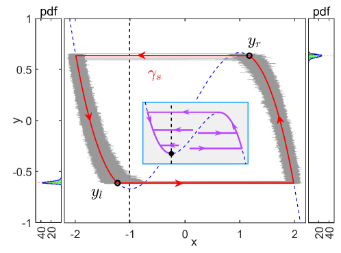
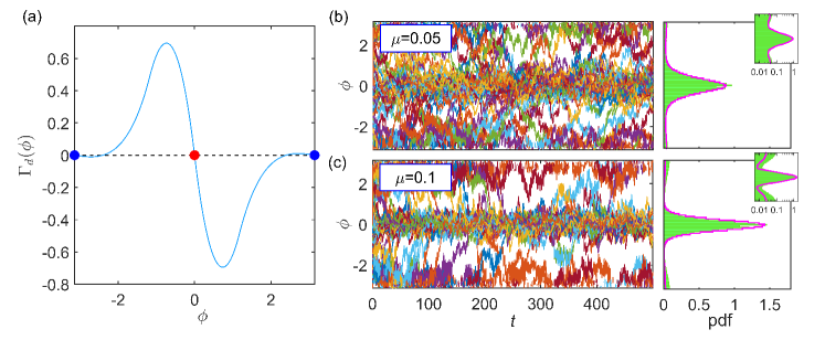
where and represent the fast membrane potential and slow recovery variable, respectively, and is the nullcline of . The Gaussian white noise satisfies and , and represents its intensity. The timescale separation parameter and the bifurcation parameter are fixed as and . Without noise, the system (1) has a globally stable fixed point (, ), where and (see the inset in Fig. 1). When noise is applied, the system (1) can exhibit noisy but coherent oscillations due to large timescale separation, called self-induced stochastic resonance (SISR) Muratov2005PD . Figure 1 illustrates the SISR oscillations observed at noise intensity . We refer to the system (1) as the SISR oscillator hereafter.
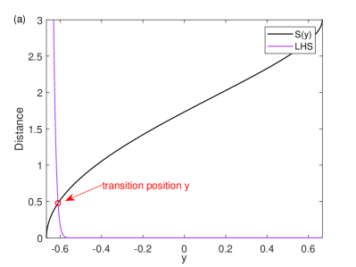
To determine the reference periodic orbit characterizing the coherent oscillations, we apply the distance matching condition (DMC) that we developed in Ref. Zhu2021PRR to calculate the transition positions (see Supplemental Material (SM) supplement for details). The transition position of the stochastic trajectory started from the initial state on the left branch can be determined from the following DMC:
| (2) |
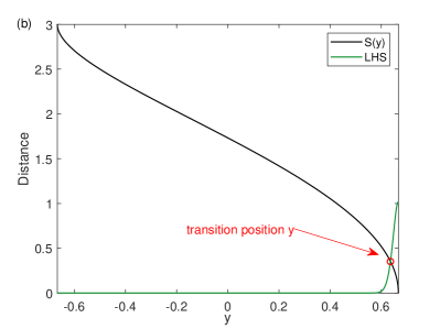
where is the value of on the left branch at and is the mean first passage time. The left-hand side of Eq. (2) represents the accumulated effect of noise on the displacement of the state away from the stable branch and on the right-hand side is the distance between the middle and left branches. This condition implies that the transition occurs when the noise-induced displacement and the distance from the left to the middle branch match. As shown in Fig. 1, the transition positions on the left and right branches predicted by Eq. (2) are in good agreement with the Monte Carlo (MC) simulations. It is found that the transition position can also be predicted by considering the first passage time distribution (FPTD) Gardiner1985 ; Lim2010JCN ; Li2019PRE , which can be calculated for the left branch (and similarly for the right branch) as supplement
| (3) |
The peak of FPTD agrees well with the transition position predicted from DMC on each branch as shown in Fig. 1.
It is noted that the stochastic oscillations caused by SISR possess a well-defined orbit and almost keep a deterministic period. These features pave the way for applying the phase reduction approach to this system. This stochastic periodic orbit is completely different from the deterministic orbit in the oscillatory regime of the system and cannot be approximated by some limiting process of the latter. In particular, the transition from one branch to the other happens before reaching the tips of the nullcline. In order to simplify our analysis, we fix the noise intensity in what follows. However, we note that the SISR phenomenon can also be induced at different noise intensities as shown in Ref. Zhu2021PRR and the proposed reduction method is generally applicable to a wide range of parameters.
Considering the fast-slow characteristics of the stochastic periodic orbit, we approximate the SISR oscillator by using the following hybrid (piecewise-continuous) dynamical system:
| (4) |
Here, , is the deterministic vector field of the system (1), are switching surfaces on the left and right branches, and are transition functions. That is, we approximate the slow stochastic dynamics along the left and right branches by the deterministic orbit of the original system and the fast dynamics between the branches by instantaneous discontinuous transitions. The transition functions and the switching surfaces can be calculated as , , and , where , , and and are the transition positions on the left and right branches obtained by DMC supplement . This system has a stable, piecewise-continuous limit cycle, denoted as , of frequency , where is nearly equal to the average frequency of the stochastic oscillations.
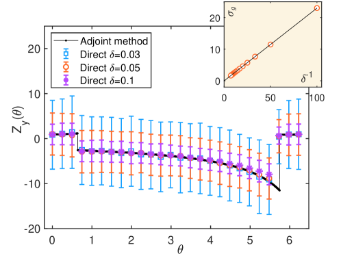
Through the above approximation, we have transformed the original stochastic system (1) to the hybrid system (4). We now apply the phase reduction method for hybrid systems Shirasaka2017PRE to further reduce the system (4) into the phase equation of the form , where is the frequency of Eq. (4) and is the phase of the system. Here, the phase function gives the asymptotic phase Winfree1980 ; Kuramoto1984 ; Nakao2016 of the state within the basin of attraction of the limit cycle . When the SISR oscillator is additionally subjected to a weak perturbation , the first-order approximate phase dynamics is given by , where we have approximated the system state by the state on sharing the same asymptotic phase, and is the phase sensitivity function of , which can be obtained via the adjoint method for hybrid limit cycles supplement . The component of the phase sensitivity functions is illustrated in Fig. 2, which has discontinuities at the two transition positions.
In the above derivation of the phase equation, we omitted the stochastic fluctuations of the SISR oscillator. To better describe the stochastic dynamical behaviors and quantitatively evaluate the accuracy of our prediction, we further incorporate the stochasticity of the system into the phase equation as an effective additive noise Schwabedal2010PRE ; Nakao2010Chaos ,
| (5) |
where denotes the effective frequency of the stochastic oscillations, is the Gaussian-white noise satisfying and , and represents the effective noise intensity. The effective frequency and noise intensity are evaluated by the ensemble average Nakao2010Chaos as and , respectively, by MC simulations of the original system (1), which are obtained as and . As discussed in SM supplement , the approximate theoretical value of the effective frequency can be obtained from DMC as and that of the effective noise intensity can be evaluated from FPTD as , which agree well with the values of and and quantitatively validate the hybrid system (4).
We can also evaluate the effective noise intensity by direct measurement of the phase sensitivity function supplement . The component of the phase sensitivity functions evaluated using several different perturbation intensities is shown in Fig. 2. As discussed in SM supplement , as the perturbation intensity used for the measurement becomes smaller, the mean value of the measured approaches the theoretical result for infinitesimal perturbation intensity calculated by the adjoint method, while its standard deviation increases as . From the inset of Fig. 2, the effective noise intensity is evaluated as , which is also consistent with the values obtained by the other methods. In the following analysis, we fix the parameters as and in the effective phase equation (5). As we will demonstrate, the simple reduced phase equation (5) that we have derived can accurately predict the dynamical behaviors of the SISR oscillator (1) under general weak perturbations, such as the periodic forcing and mutual coupling.
Periodic forcing.- We first consider a periodically forced SISR oscillator described by
| (6) |
where the forcing frequency is close to the effective frequency and characterizes the strength of the periodic forcing, which is weak in the sense that the frequency difference is given by where and is of . By applying the reduction method described above, we obtain the reduced phase equation . By further introducing the slow relative phase , we obtain Since varies much more slowly than because is of , we can average this equation via the corresponding Fokker-Planck equation over one period of fast oscillation Kuramoto1984 . This yields a further simplified phase equation
| (7) |
where is a phase coupling function representing the effect of the periodic forcing on the phase dynamics.
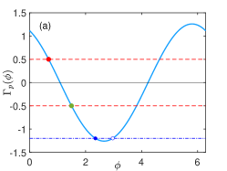
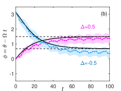
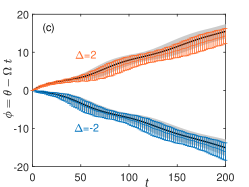
The phase coupling function is plotted in Fig. 3(a), which is smooth despite that the phase sensitivity function is discontinuous because is a convolution of with a smooth function. The solution to gives the phase-locked state and it is linearly stable (unstable) when [] if the noise is not considered. Figure 3(b) shows the time evolution of the relative phase converging to the stable phase-locked state for the cases with and . The results of MC simulations of the system (6) are in good agreement with the theoretical prediction by the noiseless phase model with the phase coupling function in Fig. 3(a). When the frequency difference is above the critical value, i.e., , the relative phase will continue to increase or decrease with time because the noiseless system does not have stable phase-locked states, and phase drift will occur Pikovsky2001book . Figure 3(c) shows that this can also be well predicted by using the reduced phase model.
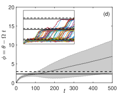
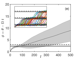
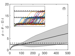
When is slightly below the critical value, noise-induced phase slipping Pikovsky2001book ; Nakao2016 ; Stankovski2012PRL ; Berglund2014ArXiv can be observed. Figure 3(d) shows the results of MC simulations of Eq. (6). The relative phase converges to the stable phase-locked state, but it can occasionally cross the unstable phase-locked state due to noise and exhibits phase slips. This phenomenon can also be well reproduced by the reduced phase equation (7) as shown in Fig. 3(e), plotting the results of MC simulations for the averaged phase model. The discrepancy of Fig. 3(e) from Fig. 3(d) mainly originates from the averaging approximation. By directly performing simulations of the reduced phase equation before averaging, the discrepancy from the original model can be significantly reduced as shown in Fig. 3(f).
Two-coupled SISR oscillators.- Next, we consider two weakly coupled identical SISR oscillators described by
| (8) |
where () represents weak coupling strength. The Gaussian white noise terms in Eq. (8) are mutually independent and satisfy and . The diffusive coupling is introduced only between the slow variables. Similarly to Eq. (7), the reduced phase equation for each oscillator is given by . By considering the phase difference , which is a slow variable, and applying the averaging procedure, we can derive the equation for as Kuramoto1984
| (9) |
where is the antisymmetric part of the phase coupling function . The solution of represents a synchronized state of the two SISR oscillators, which is stable (unstable) when []. As the two oscillators are identical and the coupling is symmetric, the in-phase () and antiphase () synchronized states are always the solutions as shown in Fig. 4(a). It is notable that both synchronized states are stable in the parameter regime considered here (although the stability of the antiphase synchronization is weaker).
Since noise is present in our coupled system (8), the phase difference does not converge to a fixed value but forms a stationary distribution with peaks corresponding to the stable synchronized states Zhu2020ND . This distribution depends on both the noise intensity and the coupling strength. We performed MC simulations of the coupled system (8) with initial phase differences uniformly distributed in . As shown in Fig. 4(b)-(c), the phase difference tends to localize around the in-phase and antiphase synchronized states. Increasing the coupling strength can enhance the localization and more clearly separate the two states, which shows the competing relationship between the coupling-induced synchronization and noise-induced desynchronization. The distributions of the phase difference obtained by MC simulations of the original system can be well reproduced by the reduced phase equation (9) with the coupling function obtained theoretically, wherein a higher peak is observed at the more stable in-phase state than at the less stable antiphase state. As expected, for smaller coupling strength, the phase-difference distribution is more accurately predicted.
Conclusion.- We have investigated the phase dynamics of the SISR oscillator exhibiting noise-induced coherent oscillations. The transition positions on each branch were accurately obtained via DMC or FPTD, and an approximate hybrid system was established by connecting the dynamics on the two slow branches by discontinuous transitions. We performed phase reduction on the hybrid system and obtained the reduced phase equation by further incorporating the effective frequency and effective noise intensity. The reduced equations were applied to the analysis of a periodically forced SISR oscillator and a pair of mutually coupled identical SISR oscillators. The good agreement between the predicted dynamics and the results of the original model proved the accuracy and efficiency of our reduction method. The analysis in this Letter can be readily extended to more complex situations such as nonidentical coupled oscillations and networks. Also, more accurate results would be obtained by considering higher-order approximations Rosenblum2019Chaos ; Leon2019PRE . Moreover, despite that the considered SISR oscillator has only one-dimensional slow dynamics, the present approach can also be extended to systems with higher-dimensional slow dynamics as long as the oscillation is coherent. More details will be reported in our future works.
Acknowledgments.- We thank the anonymous reviewers for valuable and insightful comments. J.Z. acknowledges support from JSPS KAKENHI JP20F40017, Natural Science Foundation of Jiangsu Province of China (Grant No. BK20190435), and the Fundamental Research Funds for the Central Universities (Grant No. 30920021112). Y.K. thanks JSPS KAKENHI JP20J13778 and JP22K14274 for financial support. H.N. thanks JSPS KAKENHI JP22K11919, JP22H00516, JPJSBP120202201, and JST CREST JP-MJCR1913 for financial support.
References
- (1) Ilya Prigogine. Non-equilibrium statistical mechanics. Courier Dover Publications, New York, 2017.
- (2) Werner Horsthemke and René Lefever. Noise-induced transitions: theory and applications in physics, chemistry, and biology. Springer, Berlin, 1984.
- (3) Paul C. Bressloff and Jay M. Newby. Stochastic models of intracellular transport. Reviews of Modern Physics, 85(1):135–196, 2013.
- (4) Changsong Zhou and Jürgen Kurths. Noise-induced phase synchronization and synchronization transitions in chaotic oscillators. Physical Review Letters, 88(23):230602, 2002.
- (5) Jun Nosuke Teramae and Dan Tanaka. Robustness of the noise-induced phase synchronization in a general class of limit cycle oscillators. Physical Review Letters, 93(20):204103, 2004.
- (6) Hiroya Nakao, Kensuke Arai, and Yoji Kawamura. Noise-induced synchronization and clustering in ensembles of uncoupled limit-cycle oscillators. Physical Review Letters, 98(18):184101, 2007.
- (7) Dmitri V. Alexandrov, Irina A. Bashkirtseva, Michel Crucifix, and Lev B. Ryashko. Nonlinear climate dynamics: From deterministic behaviour to stochastic excitability and chaos. Physics Reports, 902:1–60, 2021.
- (8) Benjamin Lindner, Jordi García-Ojalvo, A. Neiman, and L. Schimansky-Geier. Effects of noise in excitable systems. Physics Reports, 392(6):321–424, 2004.
- (9) Yoshiki Kuramoto. Chemical Oscillations, Waves, and Turbulence, volume 19 of Springer Series in Synergetics. Springer-Verlag, Berlin, 1984.
- (10) Hiroya Nakao. Phase reduction approach to synchronisation of nonlinear oscillators. Contemporary Physics, 57(2):188–214, 2016.
- (11) Kiyoshi Kotani, Ikuhiro Yamaguchi, Yutaro Ogawa, Yasuhiko Jimbo, Hiroya Nakao, and G. Bard Ermentrout. Adjoint method provides phase response functions for delay-induced oscillations. Physical Review Letters, 109(4):044101, 2012.
- (12) Kiyoshi Kotani, Yutaro Ogawa, Sho Shirasaka, Akihiko Akao, Yasuhiko Jimbo, and Hiroya Nakao. Nonlinear phase-amplitude reduction of delay-induced oscillations. Physical Review Research, 2(3):033106, 2020.
- (13) Hiroya Nakao, Tatsuo Yanagita, and Yoji Kawamura. Phase-reduction approach to synchronization of spatiotemporal rhythms in reaction-diffusion systems. Physical Review X, 4(2):021032, 2014.
- (14) Yi Ming Lai, Jay Newby, and Paul C. Bressloff. Effects of Demographic Noise on the Synchronization of a Metapopulation in a Fluctuating Environment. Physical Review Letters, 107(11):118102, 2011.
- (15) Jun Nosuke Teramae, Hiroya Nakao, and G. Bard Ermentrout. Stochastic phase reduction for a general class of noisy limit cycle oscillators. Physical Review Letters, 102(19):194102, 2009.
- (16) Sho Shirasaka, Wataru Kurebayashi, and Hiroya Nakao. Phase reduction theory for hybrid nonlinear oscillators. Physical Review E, 95(1):012212, 2017.
- (17) Y. Park, K. M. Shaw, H. J. Chiel, and P. J. Thomas. The infinitesimal phase response curves of oscillators in piecewise smooth dynamical systems. European Journal of Applied Mathematics, 29(5):905–940, 2018.
- (18) Eugene M. Izhikevich. Phase equations for relaxation oscillators. SIAM Journal on Applied Mathematics, 60(5):1789–1804, 2000.
- (19) Jinjie Zhu, Jiong Wang, Shang Gao, and Xianbin Liu. Phase reduction for FitzHugh-Nagumo neuron with large timescale separation. Physical Review E, 101(4):042203, 2020.
- (20) Yuzuru Kato, Naoki Yamamoto, and Hiroya Nakao. Semiclassical phase reduction theory for quantum synchronization. Physical Review Research, 1(3):033012, 2019.
- (21) Yuzuru Kato and Hiroya Nakao. Semiclassical optimization of entrainment stability and phase coherence in weakly forced quantum limit-cycle oscillators. Physical Review E, 101(1):012210, 2020.
- (22) Arthur T Winfree. The Geometry of Biological Time. Springer-Verlag, Berlin, 1980.
- (23) Seung Kee Han, Tae Gyu Yim, D. E. Postnov, and O. V. Sosnovtseva. Interacting coherence resonance oscillators. Physical Review Letters, 83(9):1771–1774, 1999.
- (24) Björn Kralemann, Laura Cimponeriu, Michael Rosenblum, Arkady Pikovsky, and Ralf Mrowka. Phase dynamics of coupled oscillators reconstructed from data. Physical Review E, 77(6):066205, 2008.
- (25) Justus T.C. Schwabedal and Arkady Pikovsky. Effective phase dynamics of noise-induced oscillations in excitable systems. Physical Review E, 81(4):046218, 2010.
- (26) Peter J. Thomas and Benjamin Lindner. Asymptotic phase for stochastic oscillators. Physical Review Letters, 113(25):254101, 2014.
- (27) Pérez-Cervera, Alberto, Benjamin Lindner, and Peter J. Thomas. Isostables for Stochastic Oscillators. Physical Review Letters, 127(25):254101, 2021.
- (28) Yuzuru Kato, Jinjie Zhu, Wataru Kurebayashi, and Hiroya Nakao. Asymptotic phase and amplitude for classical and semiclassical stochastic oscillators via koopman operator theory. Mathematics, 9(18):2188, 2021.
- (29) Cyrill B. Muratov, Eric Vanden-Eijnden, and Weinan E. Self-induced stochastic resonance in excitable systems. Physica D: Nonlinear Phenomena, 210(3-4):227–240, 2005.
- (30) Jinjie Zhu and Hiroya Nakao. Stochastic periodic orbits in fast-slow systems with self-induced stochastic resonance. Physical Review Research, 3(3):033070, 2021.
- (31) See Supplemental Material at [URL will be inserted by publisher] for prediction of stochastic periodic orbits of the excitable FHN system, phase reduction of the hybrid system, and direct method for measuring the phase sensitivity function.
- (32) Crispin W Gardiner. Handbook of Stochastic Methods: for physics,chemistry and the natural sciences. Springer-Verlag Berlin Heidelberg, 1985.
- (33) Sukbin Lim and John Rinzel. Noise-induced transitions in slow wave neuronal dynamics. Journal of Computational Neuroscience, 28(1):1–17, 2010.
- (34) Yongge Li, Yong Xu, and Jürgen Kurths. First-passage-time distribution in a moving parabolic potential with spatial roughness. Physical Review E, 99(5):052203, 2019.
- (35) Hiroya Nakao, Jun Nosuke Teramae, Denis S. Goldobin, and Yoshiki Kuramoto. Effective long-time phase dynamics of limit-cycle oscillators driven by weak colored noise. Chaos, 20(3):033126, 2010.
- (36) Arkady Pikovsky, Michael Rosenblum, and Jürgen Kurths. Synchronization: A Universal Concept in Nonlinear Sciences. Cambridge University Press, Cambridge, 2001.
- (37) Tomislav Stankovski, Andrea Duggento, Peter V.E. McClintock, and Aneta Stefanovska. Inference of time-evolving coupled dynamical systems in the presence of noise. Physical Review Letters, 109(2):024101, 2012.
- (38) Nils Berglund. Noise-induced phase slips, log-periodic oscillations, and the Gumbel distribution. Markov Process And Related Fields, 22(3):467-505, 2014.
- (39) Jinjie Zhu. Phase sensitivity for coherence resonance oscillators. Nonlinear Dynamics, 102(4):2281–2293, 2020.
- (40) Michael Rosenblum and Arkady Pikovsky. Numerical phase reduction beyond the first order approximation. Chaos, 29(1):011105, 2019.
- (41) León, Iván, and Pazó, Diego. Phase reduction beyond the first order: The case of the mean-field complex Ginzburg-Landau equation. Physical Review E, 100(1):012211, 2019.
Supplemental Material
Phase dynamics of noise-induced coherent oscillations in excitable systems
J. Zhu, Y. Kato and H. Nakao
I Stochastic periodic orbits for the excitable FHN system
For the timescale separation parameter considered in this paper, the stochastic orbits as shown in Fig. 1 in the main text are very coherent. We apply the distance matching condition (DMC), which we developed in Zhu2021PRRs , to obtain the critical transition position on the left branch of the nullcline. The calculation of the transition position on the right branch is similar.
For each fixed value of the slow variable on the left branch, there is a corresponding mean first passage time (MFPT) characterizing the difficulty of the transition from the left branch to the middle one. The MFPT can be easily obtained from Eq.(1) in the main text describing the system as Gardiner1985s
| (10) |
where represents the potential function of the deterministic fast subsystem of system (1) in the main text, and are values of on the left (stable) and middle (unstable) branches for the fixed slow variable , respectively, and is the noise intensity. The mean first passage velocity (MFPV) can be accordingly defined as
| (11) |
where is the distance between the left and middle branches, which is also a function of the slow variable . By integration with respect to time using and ( and subscript denotes the solution on the left branch) and substituting Eq.(10) into Eq.(11), the DMC is expressed as
| (12) |
where is the starting position which can be chosen arbitrarily above but not close to the final transition position (the result depends on only slightly).
By numerically evaluating the left-hand side(LHS) and right-hand side(RHS) of Eq.(12), the intersection point of these two curves gives the transition position. For the parameters considered in this paper, the results are shown in Fig. 5. It is found that the transition happens in a narrow range of and the LHS remains nearly zero initially for large , which implies that the choice of is not important as long as it is not too close to the transition position.
After determining the transition positions on the left () and right () branches, the stochastic periodic orbit can be obtained by connecting the slow dynamics along the nullcline with the jump processes at the transition positions (see Fig. 1 in the main text). The period can thus be approximated as
| (13) |
Therefore, the frequency of the hybrid system can be obtained as , which approximates the average frequency of the SISR oscillator.
To estimate the dispersion of the stochastic periodic orbit, we can consider the first passage time distribution (FPTD) Gardiner1985s ; Lim2010JCNs ; Li2019PREs . For fixed , the survival probability that the state remains on the LHS of the middle branch can be defined as
| (14) |
where is the first passage time for the state escaping from the middle branch for fixed . The derivative of the escape probability with respect to gives the FPTD . Thus, the escape rate satisfies:
| (15) |
Note that the escape rate is just the reciprocal of the MFPT, so that the survival probability can be easily solved as
| (16) |
Therefore, we can obtain the FPTD as
| (17) |
Replacing with and by noting , we can finally achieve our derivation for the FPTD as a function of :
| (18) |
The FPTD on the right branch is similar:
| (19) |
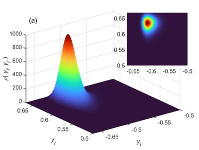
The FPTDs on the left and right branches are shown in Fig. 1 in the main text, which are consistent with the results by Monte Carlo simulations. Assuming that the transition positions on the left and right branches are independent, the joint probability density of the transition positions is given by
| (20) |
The joint probability density shown in Fig. 6(a) exhibits a clear peak at the transition positions, which is consistent with the coherent oscillations. Using Eq.(13), the oscillation frequency with different transition positions can be calculated as in Fig. 6(b). Finally, we can approximate the mean and variance of as
| (21) |
The effective noise intensity can thus be approximated as
| (22) |
Therefore, via numerical calculation of the above equations for the parameter values used in the main text, the effective frequency and effective noise intensity can be estimated as and ( in the main text), which are close to the evaluated values via Monte Carlo simulations in the main text.
The small errors in the estimation of and can be explained as follows. It can be observed that nearly all stochastic trajectories on the left branch undergo transitions before the tip of the nullcline, while the transitions on the right branch can happen after the tip with a finite probability (see the inset of Fig. 6(a) for a blowup where the upper part is slightly truncated). This truncated probability can be quantitatively measured by integrating the joint probability density within the considered area, which gives . Although the distribution above the tip of the nullcline cannot be calculated within the framework of FPTD, it can be inferred that the lack of those trajectories will make the estimated effective frequency larger and effective noise intensity smaller, which contributes to the errors in our estimation.
II Phase reduction of the hybrid system
We consider a hybrid system defined as follows (Eq.(4) in the main text):
| (23) |
where represents the transition function and is the switching surface (for the left and right branches). Considering the large timescale separation, we assume that, when the state crosses the critical transition position, it will be instantly attracted to the other stable branch of the nullcline, so that and , where (solving the cubic equation by using the trigonometric functions). We assume that Eq.(23) has a stable piecewise-continuous limit-cycle solution , and introduce an asymptotic phase function in its basin of attraction. We denote this limit cycle as and introduce the phase variable of the system as , which increases with a constant frequency in the absence of perturbations. The state of is expressed as as a function of the phase. Applying the phase reduction method for hybrid systems on system (23) under a weak perturbation , the reduced equation can be given as
| (24) |
where we have approximated by the state on having the same phase value as and is the phase sensitivity function of .
The phase sensitivity function can be obtained by solving the following adjoint system Shirasaka2017PREs for hybrid limit-cycle oscillators:
| (25) |
with the normalization condition:
| (26) |
Here, is the Jacobi matrix of at and the superscript denotes transpose. The saltation matrix describing the change in at the switching surface is given by Shirasaka2017PREs :
| (27) |
where is the Jacobi matrix of and denotes the transition time. The symbol represents the Kronecker product. Through backward integration, the adjoint equation (25) can be numerically solved Ermentrout2010Books ; Ermentrout1996NCs . For details of the phase reduction approach on the hybrid system, the readers are referred to Ref. Shirasaka2017PREs .
III Direct method for phase sensitivity function
For deterministic systems with a stable limit cycle, a fixed perturbation at a fixed timing can produce a fixed change of the phase value. The phase response function characterizing the change of the phase value caused by a perturbation given at the phase can be represented as
| (28) |
By assuming the perturbation to be small, the following Taylor expansion can be obtained:
| (29) |
where is the phase sensitivity function. Therefore, by applying a sufficiently small perturbation ( is a unit vector with only a single nonzero value at its -th component), the -th component of the phase sensitivity function can be numerically measured as
| (30) |
The phase value of can be calculated by evolving the state for several periods of the oscillator until it converges to the stable limit cycle. However, for the SISR oscillator, the phase value differs between realizations due to noise. We denote by and the oscillator states at time with initial conditions and . Then, according to Eq.(5) in the main text, the corresponding phase values evolve as
| (31) |
where and are independent Wiener processes. From Eq.(29), the following time-dependent stochastic phase response is obtained:
| (32) |
where is another Wiener process. By introducing a phase response function rescaled by the perturbation strength as , the -th component of can be expressed as
| (33) |
where we used . The standard deviation of is . Therefore, we can also measure the effective noise intensity from . It is interesting to see that there is a dilemma here: decreasing the perturbation strength can increase the linearity and thus the accuracy of the phase sensitivity function computed by the above direct method, making it closer to the theoretical result obtained via the adjoint method for the hybrid system; while it may also increase the standard deviation of the result, which may make the simulation results more stochastic. This dilemma can be observed in Fig. 2 in the main text.
References
- (1) Jinjie Zhu and Hiroya Nakao. Stochastic periodic orbits in fast-slow systems with self-induced stochastic resonance. Physical Review Research, 3(3):033070, 2021.
- (2) Crispin W Gardiner. Handbook of Stochastic Methods: for physics,chemistry and the natural sciences. Springer-Verlag Berlin Heidelberg, 1985.
- (3) Sukbin Lim and John Rinzel. Noise-induced transitions in slow wave neuronal dynamics. Journal of Computational Neuroscience, 28(1):1–17, 2010.
- (4) Yongge Li, Yong Xu, and Jürgen Kurths. First-passage-time distribution in a moving parabolic potential with spatial roughness. Physical Review E, 99(5):052203, 2019.
- (5) Sho Shirasaka, Wataru Kurebayashi, and Hiroya Nakao. Phase reduction theory for hybrid nonlinear oscillators. Physical Review E, 95(1):012212, 2017.
- (6) Ermentrout, G. Bard and Terman, David H. Mathematical Foundations of Neuroscience. Springer New York Dordrecht Heidelberg London, 2010.
- (7) Ermentrout, Bard. Type I Membranes, Phase Resetting Curves, and Synchrony. Neural Computation, 8(5):979–1001, 1996.