Phase space deformations in phantom cosmology.

One of the most intriguing aspects in physics, is the current acceleration of the Universe. Is it a consequence of modifications to general relativity (GR) or is it a new kind of matter that drives this acceleration?. Although having some theoretical problems, the best answer to this question is the cosmological constant $\Lambda$. An alternative candidate that has been successful for the description of dark energy is the scalar field [1, 2, 3, 4, 5, 6]. In particular, scalar fields with a negative kinetic term have been considered in the literature. This type of fields are known as Phantom fields. They have some interesting properties that allows them to be considered as a strange but viable matter which could be relevant in the evolution of the Universe [7]. In particular, a phantom field provides an effective negative pressure and a repulsive effect on the matter content of the Universe which in the long term could be responsible for the current accelerated expansion [8, 9, 10, 11, 12]. Therefore it has been considered as the matter source of the late time accelerated expansion of the Universe [13, 14, 15].

When considering the spacetime structure of the Universe it is usually done in reference to GR. But when regarding the micro structure of spacetime we do not have a universally accepted quantum theory of gravity. Although there are several candidates, noncommutativity has been considered as an alternative to understand the small scale structure of the Universe and help in the construction of quantum theory of gravity. For this reason, noncommutative versions of gravity have been constructed [16, 17, 18, 19]. Noncommutativity is usually believed to be present near Planck’s scale and is consistent with a discrete nature of spacetime. Motivated by this idea, it is justified to consider an inherently noncommutative spacetime at the early ages of the universe. Directly using noncommutative gravity is quite difficult, this is a consequence of the highly nonlinear character of these theories[16, 17, 18, 19]. Fortunately there is an alternative, in [20] the authors introduce the effects of noncommutativity using the Moyal product of functions on the Wheeler-DeWitt (WDW) equation.
The effects of the noncommutative deformation at the classical level was studied by a WKB approximation of noncommutative quantum model [21] and also by modifying the Poisson algebra [22, 23]. More general minisuperspace deformations have been done in connection with $\Lambda$ [24, 25, 26, 27, 28, 29]. Phase space deformations give rise to two physically nonequivalent descriptions, the “C-frame” based on the original variables but with a modified interaction and the “NC-frame” frame based on the deformed variables but with the original interaction. Given this ambiguity, in [29] a principle was proposed to restrict the value of the deformation parameters in order to make both descriptions physically equivalent.

In this work we consider a Friedmann-Robertson-Walker (FRW) cosmological model coupled to a phantom scalar field and study the physical consequences of introducing general phase space deformations on the minisuperspace of the theory. We will study both, the classical and quantum models and we also find that the semiclassical approximation of the deformed quantum model agrees with the classical model. The deformation parameter space is determined by considering the principle of physically equivalent frames [29].

The paper is organized as follows. In section 2, the commutative model is presented. In section 3, the minisuperspace phase space deformation is implemented and the dynamics in the two frames is obtained. Also the deformation parameters are constrained by imposing physical equivalence between the “C-frame” and the “NC-frame”. The quantum analysis is done in section 4, we find the solution to the deformed WDW equation and fix the parameters in the deformation in order to make the quantization possible. We also show that the classical paths arise from the semiclassical approximation of the WDW equation obtained from the deformed Hamiltonian. Finally, section 5 is devoted for concluding remarks.

We start with the flat FRW metric

$a(t)$ corresponds to the scale factor and $N(t)$ is lapse function. In this background the action of a minimally coupled phantom scalar field $\varphi(t)$ with constant potential is

where we have set the units so $8\pi G=1$. The minus sign in the kinetic term of the scalar action is the difference between the usual scalar field and the phantom scalar field [12]. The canonical Hamiltonian derived from Eq.(2) is

With the the following change of variables

and $\mu=\sqrt{3/8}$. The Hamiltonian Eq.(3) can be rewritten as a sum of two harmonic oscillators

where $\omega^{2}=-\frac{3}{4}\Lambda$. When one considers the usual scalar field, the Hamiltonian is transformed to a “ghost oscillator” which is simply a difference of two harmonic oscillators [26, 29].

There exist different approaches to incorporate noncommutativity into physical theories. Particularly, in cosmology there is a broadly explored path to study noncommutativity [20], where noncommutativity is realized in the so called minisuperspace variables. We will follow a deformed phase space approach. The deformation is introduced by the Moyal bracket $\{f,g\}_{\alpha}=f\star_{\alpha}g-g\star_{\alpha}f$. By substituting the usual product with the Moyal product $(f\star{g})(x)=\exp{\left[\frac{1}{2}\alpha^{ab}\partial_{a}^{(1)}\partial_{b}^{(2)}\right]}f(x_{1})g(x_{2})|_{x_{1}=x_{2}=x}$ such that

The $2\times 2$ antisymmetric matrices $\theta_{ij}$ and $\beta_{ij}$ represent the noncommutativity in the coordinates and momenta respectively. The $\alpha$ deformed algebra becomes

In this work we use the particular deformations, $\theta_{ij}=-\theta\epsilon_{ij}$ and $\beta_{ij}=\beta\epsilon_{ij}$.

To construct the deformed theory, we start with a Hamiltonian which is formally analogous to Eq.(5) but constructed with the variables that obey the modified algebra Eq.(11), this gives the deformed Hamiltonian

where $\ell^{2}$ and $\widetilde{\omega}^{2}$ are given by

There is a significant difference between the transformed Hamiltonian of the scalar field cosmology model [26] and Eq. (12), the deformed Hamiltonian of the phantom cosmology model. Unlike the scalar field case, the crossed term involving position and momentum in the phantom model, corresponds to an angular momentum term. To understand the physics of the deformation, it is necessary to remember that the deformation Eq.(10) defines two physical nonequivalent descriptions, the “C-frame” where the effects of the deformation are interpreted as a commutative space $(x,y)$ but with modification of the original interaction and the “NC-frame” where we work with the deformed variables $(\widehat{x},\widehat{y})$ and the original interaction. In general, the dynamics in the two frames is different but the physical interpretation in the “C-frame” is easier. In this frame we can interpret the deformed model as a bidimensional harmonic oscillator and the minisuperspace deformation comes into play as an angular momentum term in the Hamiltonian. For this reason we will do the calculations in the “C-frame”.

We obtain the equations of motion from the Hamiltonian Eq.(12), which in the $(x,y)$ variables are given by

and get

With the transformation $z=x+iy$ we can easily solve Eq.(15). We have three different solutions depending on the sign of $\widetilde{\omega}^{2}$. For $\widetilde{\omega}^{2}>0$, we get

$A_{1},B_{1}$ are arbitrary constants that, from the Hamiltonian constraint, satisfy $(\ell^{2}+2|\widetilde{\omega}|)A_{1}-(\ell^{2}-2|\widetilde{\omega}|)B_{1}=0$. When $\widetilde{\omega}^{2}<0$ we have the solutions

for this case the integrating constants satisfy the condition $A_{3}^{2}=B_{3}^{2}$. The last solution is for the case $\widetilde{\omega}=0$,

the constraint imposes $B_{2}=0$. The condition arises when the cosmological constant satisfies $2\beta=-3\Lambda$.

In analyzing the evolution of the Universe, we will focus our attention on its volume and calculate $a^{3}(t)$ in the two frames. Let us start in the “C-frame”, using the solutions for the model, Eq.(16), Eq.(17) and Eq.(18), together with the change of variables in Eq.(4) we get

where $V^{(i)}_{0},V^{(i)}_{1}$ are constructed from the integrating constants. For the first case, $V^{(1)}_{0}=(A_{1}-B_{1})^{2}$ and $V^{(1)}_{1}=4A_{1}B_{1}$, we must remember that the constants are related. For the second case the volume is the square of a constant. Finally for the last case we have $V^{(3)}_{0}=A_{3}^{2}$, but if we take $A_{3}=-B_{3}$ we have an exponentially decaying volume.

To study the dynamics in the “NC-frame” we use the “C-frame” solutions. The volume is constructed with the “NC-frame” variables, $\widehat{a}^{3}(t)=m^{2}(\widehat{x}^{2}+\widehat{y}^{2})$

where $\widehat{V}^{(i)}_{0},\widehat{V}^{(i)}_{1}$ are constants related to $V^{(i)}_{0},V^{(i)}_{1}$. It is important to mention that even if we have a positive volume in the “C-frame” we might need to impose some restriction in order to have a valid description in the “NC-frame”. In order to determine the valid range of the deformation parameters we use the principle used in [29] which states the following, “Deformed phase space models are only valid when the NC-frame and C-frame descriptions are physically equivalent”. To impose that the description in the two frames should be physically equivalent, we start by analyzing the expression for the “C-frame” volume. It is easy to show that the volume is always positive. In the first case one obtains that $V^{(1)}_{0}+V^{(1)}_{1}=(A_{1}+B_{1})^{2}\geq 0$ so is positive for any $t$. For the second case the volume is also positive, and finally for the third case the constant $V^{(3)}_{1}>0$. Then we conclude that for the three cases, the “C-frame” volume is always positive for any choice of the integration constants. The constants in the “NC-frame” solutions are related to the “C-frame” constants as follows. For the first case, $\widehat{A}_{1}=(1+|\widetilde{\omega}|\theta/2)A_{1}$ and $\widehat{B}_{1}=(1-|\widetilde{\omega}|\theta/2)B_{1}$, for the second case the volume is the same and for the last case the constant in the “NC-frame” is related by $\widehat{A}^{2}_{3}=(1+\tilde{\omega}^{2}\theta^{2}/4)A_{3}^{2}$.

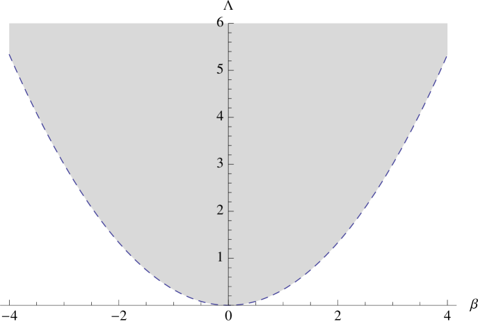
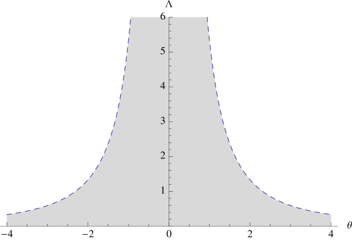
This effective cosmological constant is determined by the deformation parameters as well as the value of $\Lambda$. Since current observations point to a positive cosmological constant. This gives and extra condition that restricts the values of the deformation parameters by imposing that $\Lambda_{eff}>0$. After fixing the value of $\Lambda$, we have three definite restrictions:

1. i)

   $\Lambda_{Eff}>0$.

2. ii)

   $f(\beta,\Lambda)=3\Lambda-\beta^{2}$ and $g(\theta,\Lambda)=1-\frac{3\theta^{2}\Lambda}{16}$ must have the same sign.
   

3. iii)

   $1+\frac{\theta^{2}\widetilde{\omega}^{2}}{4}>0$.

From ii), we can see in Fig.(1) and Fig.(2) the regions where these inequalities are satisfied. We did not consider $\Lambda\leq 0$, since condition ii) would not be satisfied, for this reason the plots only show the region where $\Lambda>0$.

Now we proceed with the quantization of the deformed Hamiltonian. The usual canonical quantization approach $H_{nc}\psi=0$, gives the corresponding WDW equation. The Hamiltonian $H_{nc}$, explicitly contains the angular momentum operator $(xP_{y}-yP_{x})=L_{z}$ and can be written in terms of the Hamiltonian of a 2-dimensional harmonic oscillator $H_{xy}$, with frequency $\widetilde{\omega}^{2}$ plus an angular momentum term, that is $H_{nc}=H_{xy}+L_{z}$. Using the similarity of the WDW equation, with the 2-dimensional harmonic oscillator, we will follow the approach in [30, 31]. First we write the eigenvalue equation for the harmonic oscillator, then we will find the energy eigenvalues and finally impose the zero energy condition. After writing the quantum equation in polar coordinates, we obtain the equation for the energy eigenstates, and is given by

It is well known that the Hamiltonian of the 2d harmonic oscillator commutes with the angular momentum. This means that we have $[H_{xy},L_{z}]=0$, allowing us to write the wave function with eigenstates common to both operators. This breaks the degeneracy in energy eigenstates and every state is uniquely specified by the quantum numbers $n$ and $m$. Solving Eq.(22) we find the wave function of the Universe $\psi_{n,m}(r,\phi)$

where $n=0,1,2,...\>;~m=0,\pm 1,\pm 2,...,\pm n,$ and $L_{n}^{\alpha}(z)$ are the generalized Laguerre polynomials. The zero energy condition $E=0$ from the WDW equation is trivially satisfied by $\ell=\widetilde{\omega}=0$. For $\ell\neq 0,~\widetilde{\omega}\neq 0$ (for instance for a single state of quantum numbers $n$ and $m$) we get the general equation

By using the definitions for $\ell^{2}$ and $\widetilde{\omega}^{2}>0$ we can write this equation as

With respect to the condition in Eq. (25), we need to find the values of $\theta$, $\beta$ and $\Lambda$ to satisfy the condition. The first thing to notice is that the right hand side of this equation takes only discrete values and to determine if there are possible values of the parameters to satisfy the equation we may proceed as follows. Analyze the behavior of the function $h(\theta,\beta,\Lambda)=\frac{16\beta-12\theta\Lambda}{\sqrt{16-3\theta^{2}\Lambda}\sqrt{4\beta^{2}-12\Lambda}}$ and then see whether or not, there are permitted values of the parameters for which the function takes the value $h(\theta,\beta,\Lambda)=-\frac{2(2n+|m|+1)}{m}$. The quantum solution is possible when $\widetilde{\omega}^{2}>0$, which corresponds to the first solution in Eq. (LABEL:CVolume) and Eq.(LABEL:NCVolume). Therefore, the space of parameters is already depicted in Fig.(1) and Fig.(2), corresponding to the condition that the functions $f(\beta,\Lambda)$ and $g(\theta,\Lambda)$ have opposite sign. The valid values of parameters $\theta$, $\beta$ and $\Lambda$, corresponds to the gray region of Fig. 1 and white region of Fig. 2, or vice versa. We use the inverse transformation of Eq.(4) with Eq. (23)

to find the wave function $\psi_{n,m}(a,\varphi)$ in terms of the scale factor $a$ and the phantom field $\varphi$.

with $m$ fixed and $c_{n,m}$ arbitrary constants as long as the condition $E=\sum_{n}^{N}E_{(n,m)}=0$ also holds. When this is the case, it is always possible to find values of $\theta$, $\beta$ and $\Lambda$ to satisfy the constriction Eq. (24), under which these values are fixed unambiguously. For a given value of $m$, the sum in Eq.(27) runs over odd/even values of $n$ depending on the odd/even value of $m$ respectively. The wave packet is normalizable by the use of the orthogonality relation of generalized Laguerre polynomials. The total energy of the wave packet will satisfy the generalized zero energy condition Eq.(24), but replacing $n$ by $N$. From the arguments given above, we conclude that it is always possible to find, for a given $\Lambda>0$ values for $\theta$ and $\beta$ for which the condition holds.

In this paper we have studied the effects of the minisuperspace phase space deformations in the dynamics of phantom scalar cosmology. The deformation was applied on the minisuperspace variables. From the deformed Hamiltonian we derived the equations of motion. It is known that from the deformation two generally nonequivalent descriptions arise. Using the solutions to Eq.(15), we calculate the volume of the Universe in the “C-frame” and in the “NC-frame”. To constrain the deformation parameters $\beta$ and $\theta$, we impose that for phase space deformations to be valid, the physical description in the two frames must be equivalent. From the value of $\widetilde{\omega}^{2}$ three different cases appear. For $\widetilde{\omega}^{2}>0$, we get a bouncing Universe and the solutions in the two frames are equivalent. For the last case, when the Hamiltonian constraint is applied, we have a de Sitter Universe and the parameter $\widetilde{\omega}^{2}$ can be interpreted as an effective positive cosmological constant $\Lambda_{Eff}$. The value of $\Lambda_{Eff}$ depends on the deformation parameters $\theta$ and $\beta$ as well as the original $\Lambda$. If we set the original cosmological constant $\Lambda=0$, then $\widetilde{\omega}^{2}>0$ and is not possible to have $\Lambda_{Eff}\geq 0$. This imposes a stronger restriction on the values of $\beta$ and $\theta$ and the parameter space is even more restricted, but even when this is the case we have a region of values where the two descriptions are physically equivalent.

We quantized the model, obtaining the corresponding WDW equation and found the wave function of the Universe. We derived a relation that fixes the values of the parameters $\theta$, $\beta$ and $\Lambda$ in order to satisfy the zero energy condition of the WDW equation. We showed that the deformed phantom cosmological model is physically viable. Also, when $\widetilde{\omega}^{2}>0$ the quantization can be achieved and the introduction of the deformation breaks the degeneracy of the quantum states. A general condition on the parameters $\theta$ and $\beta$ arises from the zero energy condition that can be satisfied by the general wave packets. It is worth to mention that there is a nice physical interpretation in the “C-frame”. It is related to the introduction to an effective perpendicular and constant “magnetic field” $\vec{B}$. This can be seen by taking the bidimensional harmonic oscillator coupled to the vector potential $\vec{A}=(\frac{B}{2}y,-\frac{B}{2}x)$ where the magnitude of the field will be $B=\ell^{2}$. Then we can see that the zero energy condition is related to the manipulation of this field and corresponds to a modification in the deformation parameters $(\theta,\beta)$. Finally, we performed the WKB approximation and show that the same classical solutions arise in the classical limit of the WDW equation of the corresponding deformed Hamiltonian.

This work is supported by CONACyT research grants 167335, 257919, 258982.

References

- [1] B. Ratra and P. J. E. Peebles, Phys. Rev. D 37 3406 (1988).
- [2] P. J. E. Peebles and B. Ratra, Rev. Mod. Phys. 75, 559 (2003).
- [3] L. P. Chimento and A. S. Jakubi, Int. J. Mod. Phys. D 5 71 (1996).
- [4] E. J. Copeland, M. Sami, and S. Tsujikawa, Int. J. Mod. Phys. D 15 1753 (2006).
- [5] K. Bamba, S. Capozziello, S. Nojiri, and S. D. Odintsov, Astrophys. Space. Sci. 342 155 (2012).
- [6] T. Padmanabhan and T. Roy Choudhury, Phys. Rev. D 66 081301 (2002).
- [7] V. A. Rubakov, Theor. Math. Phys. 149 1651 (2006).
- [8] S. Perlmutter et al. [Supernova Cosmology Project Collaboration], Astrophys. J. 517, 565 (1999).
- [9] A. G. Riess et al., Astron. J. 116 1009 (1998).
- [10] A. G. Riess et al, Astrophys. J. 560 49 (2001).
- [11] Narciso Benitez et al., Astrophys. J. 577 L1 (2002).
- [12] Mariusz Dabrowski, Phys. Rev. D 74 044022 (2006).
- [13] Robert R. Caldwell and Marc Kamionkowski, Ann. Rev. Nucl. Part. Sci. 59 397 (2009).
- [14] J. M. Cline, S. Jeon, and G. D. Moore, Phys. Rev. D 70 043543 (2004).
- [15] W. Hu, Phys. Rev. D 71 047301 (2005).
- [16] H. Garcia-Compean, O. Obregon, C. Ramirez, and M. Sabido, Phys. Rev. D 68 045010 (2003).
- [17] X. Calmet and A. Kobakhidze, Phys. Rev. D 72 045010 (2005).
- [18] P. Aschieri, M.Dimitrijevic, F.Meyer and J.Wess, Class. Quant. Grav. 23 1883 (2006).
- [19] T. Ohl and A. Schenkel, JHEP 0910 052 (2009).
- [20] H. Garcia-Compean, O. Obregon, and C. Ramirez, Phys. Rev. Lett. 88 161301 (2002).
- [21] E. Mena, O. Obregon and M. Sabido, Int. J. Mod. Phys. D 18 (2009) 95.
- [22] L. O. Pimentel and O.Obregon, Gen. Rel. Grav. 38 553 (2006).
- [23] C. Bastos, O. Bertolami, N. Costa Dias and J. Nuno Prata, Phys. Rev. D 78 (2008) 023516.
- [24] B. Vakili, C. I. Azad, P. Pedram, and S. Jalalzadeh, Phys. Lett. B 687 119 (2010).
- [25] B. Malekolkalami, K. Atazadeh and B. Vakili, Phys. Lett. B 739, 400 (2014).
- [26] S. Pérez-Payán, M. Sabido and C. Yee-Romero, Phys. Rev. D 88 027503 (2013).
- [27] M. Sabido and C. Yee-Romero, Phys. Lett. B 757 (2016) 57.
- [28] A. Crespo-Hernandez, E. A. Mena-Barboza and M. Sabido, Entropy 19, 91 (2017).
- [29] Sinuhe Pérez-Payán, M. Sabido, E. Mena and C. Yee-Romero, Adv. High. Energy Phys. 2014 958137 (2014)
- [30] S. S. Gousheh and H. R. Sepangi, Phys. Lett. A 272, 304 (2000).
- [31] S. Jalalzadeh, F. Ahmadi and H. R. Sepangi, JHEP 0308, 012 (2003).