Phase transition in non-Markovian animal exploration model with preferential returns

Introduction. Movement is a vital part of life and is key in a wide range of physical, biological and ecological systems. Theoretical and empirical frameworks are thus amply used to study the mechanisms underlying movement patterns in all organisms [1]. In particular, individual-based modeling of movement has played a crucial role in studying dynamic systems across multiple spatiotemporal scales [2, 3, 4]. These models can be applied to infer behaviors and draw causal links between observed phenomena and their underlying mechanisms beyond phenomenological description of the observed patterns [5].

Most theoretical models rely on Markovian assumptions to capture the properties of animal trajectories. However, memory and similar cognitive mechanisms are key to understanding patterns observed in animal foraging [6, 7]. A range of taxa, from insects to primates, have been shown to exhibit spatial memory, and many of them are known to repeatedly return to previously visited sites as a part of their regular foraging strategies, mammals being a paradigmatic example [8, 9, 10, 11, 4]. Notably, memory patterns must be properly balanced by the organisms with some level of behavioral plasticity to enhance flexibility and exploration (see, e.g., [12]). For all these reasons, correctly incorporating memory within stochastic models is an important research line for improving both predictive and descriptive tools of movement [13, 14, 6, 15]. Indeed, it has been shown that heuristic models of memory can be derived from microscopic consideration for limited cases [16, 17]. At the same time, new experimental methods are allowing to disentangle, even under field conditions, memory effects on movement from other cognitive/perception mechanisms [9]. As long as such experimental and theoretical advances are able to nourish each other, new levels of detail in our understanding of living organisms can be potentially reached.

Dealing with memory and similar cognitive mechanisms still represents a significant theoretical challenge. Stochastic models that allow the individual to return to its original position (resettings) have attracted much attention recently [18, 19, 20], but these only incorporate memory in an elementary way. More complex self-avoiding random walks or preferential returns (PR), where the individual returns to any previous location with a probability proportional to the number of previous visits have also been studied [21, 22]. These models are non-Markovian (and typically also non-stationary), requiring that the individual identifies and keeps record of its entire trajectory. While the propagator of these models [23], and some properties of relocation times [24], have been computed, characterizing the revisits complete statistics to each particular location remains an open problem.

Here we study a non-Markovian and non-stationary mechanistic model of animal mobility, explicitly incorporating both the tendency of an individual to return to previously visited locations (PR) and the tendency to explore new sites. Versions of this model have been used to model the mobility of humans [21] and monkeys [25], the latter suggesting that monkey movements are non-random due to the use of memory and visitation patterns driven by resource availability. We generalize the model by accounting for stochasticity, incorporating inter-specific variability in the population, and allowing for nonlinear PR [26]. We provide analytical solutions to this non-Markovian, non-stationary model that go well beyond previous mean-field results. In particular, we present several approaches to analytically find the (non-stationary) probability of having visited $n$ sites at time $t$ and study the statistics of how revisits are distributed through the available locations. Our approach, based on the WKB (Wentzel–Kramers–Brillouin) approximation, is thus useful to deal with explicitly time-dependent and non-stationary problems. Remarkably, by allowing for nonlinear PR we find a phase transition as a function of the strength of the PR, where above some threshold the most visited site dominates the dynamics, receiving practically all new visits. We suggest that this phase transition reflects a balance between the tendency to return to known sites and the will to explore new ones [19]. We further verify our predictions using simulations, and show that our theoretical results adequately describe the space use patterns and the revisitation dynamics of Egyptian fruit bats (Rousettus aegyptiacus) to fruit trees.

Model. Our model consists of two elements [21]: (i) exploration – with probability $P_{new}$ the animal visits a new site, and (ii) PR – with probability $1-P_{new}$ the animal visits a previously visited site $i$ with probability $\Pi_{i}(m_{i})$, where $m_{i}$ is the number of previous visits to site $i$. Following empirical evidence in humans and animals [21, 25] we assume that

Here $n$ is the number of previously visited sites, and $\beta>0$ and $0<q<1$ control the animal’s tendency to visit new sites indicating a power-law decay controlled by conformity exponent $\beta$. On the other hand, the PR exponent $\alpha>0$, governs the tendency to return to a previously visited location. Furthermore, and without loss of generality, we order the sites by rank such that $i=1$ is the most visited site with $m_{1}$ visits. Notably, we assume that the number of available sites is always larger than the number of visited sites, and that no significant resource depletion within a site occurs.

Cumulative number of sites. The probability $P(n,t)$ of having visited $n$ sites in $t\gg 1$ time steps follows

Although this master equation is interpreted here in the context of movement between spatially distributed sites, it can equivalently describe a birth-death process of population of size $n$, where the growth rate is proportional to $n^{-\beta}$ ¹¹1Similar growth rates appear in self-inhibitory gene regulatory networks, where a protein inhibits its own growth, see e.g., Refs. [47, 48]. In particular, for $\beta=0$ the birth-death process is $\emptyset\xrightarrow{q}A$ and for $\beta=-1$ the birth-death process is $A\xrightarrow{q}2A$. While these special cases have known exact solutions, in this manuscript we are primarily interested in the regime $\beta>0$, which describes a growth which decreases [or saturates, see Eq. (1)] with the number of sites (or with the population size). To the best of our knowledge this regime has not been analytically studied.

An equation for the first moment $\left<n\right>=\sum_{n}nP(n,t)$ can be obtained from Eq. (2) by multiplying the latter by $n$, summing over all $n$’s, and using the definition for $\left<n\right>$, resulting in $d\left<n\right>/dt=q\left<n^{-\beta}\right>$ which under the mean-field approximation $\left<n^{-\beta}\right>\simeq\left<n\right>^{-\beta}$ is solved by [21]

predicting a power-law dependence on the time of measurement. A similar derivation for the second moment yields $\left<n^{2}\right>=\left<n\right>^{2}+\left<n\right>$ such that the variance follows $\sigma_{n}^{2}\equiv\left<n^{2}\right>-\left<n\right>^{2}=\left<n\right>$, i.e., the variance of the number of sites is equal to the mean as in a Poisson process. This result, however, turns out to be inaccurate as it involves various uncontrolled assumptions, and is not consistent with simulations, as elaborated below.

An exact solution to Eq. (2) can be found by Laplace transforming the equation and solving the resulting recurrence equation ²²2In the SI, Sec. S1.B we alternatively develop a a generating function approach, and Eq. (2) becomes a fractional integro-differential equation, which is solvable in specific cases.. The exact solution for $\beta\neq 0$ has the form [see Supplementary Information (SI) Sec. S1.A]

For special values of $\beta$ this result simplifies to

Although Eq. (4) is an exact solution, it is given in form of a summation of large terms of alternating sign, which converges due to a precise balance between the terms. Thus, in practice this result is very slow to converge for $n\gg 1$ in any finite-size system (e.g., python, matlab, and mathematica) and may result in a significant lack of accuracy. Moreover, virtually any approximation made in calculating the individual terms may cause large errors for $n\gg 1$ [29]. To circumvent these issues, we develop a time-dependent WKB approximation.

Time dependent WKB. In the limit of a large number of sites $n\gg 1$ [30, 31, 32], we substitute the time-dependent ansatz $P(n,t)\sim e^{-{\cal S}(n,t)}$ into Eq. (2). Neglecting terms of order $\mathcal{O}(n^{-1})$ we obtain a classical Hamilton-Jacobi equation for the action function ${\cal S}(n,t)$: $\mathcal{\partial}_{t}{\cal S}=H(n,\mathcal{\partial}_{n}{\cal S})\equiv H(n,p)$ where we have defined the Hamiltonian $H(n,p)=q\left(1-e^{-p}\right)n^{-\beta},$ and denoted $p=-\mathcal{\partial}_{n}S$ as the conjugate momentum. Instead of directly solving the Hamilton-Jacobi equations, we use the Hamilton approach for the classical equations of motion

We write the action on a classical trajectory as  [31]:

where the energy $E\equiv H[n(t),p(t)]$ is constant along a dynamical trajectory given by $p(n)=\log\left[q/(q-En^{\beta})\right]$. To find the energy we solve the equation of motion (6) on a given dynamical trajectory on which the energy is constant. After some algebra (SI, Sec. S1.C) this yields

with $x\equiv n/\left<n\right>$ and $f(x)=1-x^{\beta}(\beta(x-1)+x)$. Here, $B(z;a,b)=\int_{0}^{z}u^{a-1}(1-u)^{b-1}du$ is the incomplete beta function. This calculation of the probability of having visited $n\gg 1$ sites at time $t$, is one of our main results. In the low energy limit, $E\ll 1$, $S(x)$ becomes (SI)

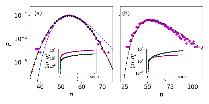
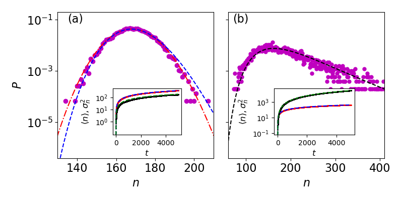
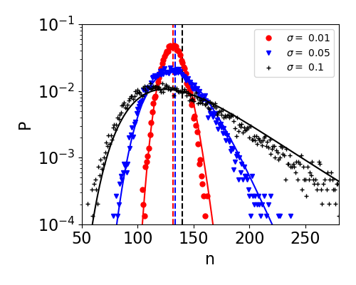
which can be shown to solve the Hamilton-Jacobi equation in the limit $|x-1|\ll 1$. In Fig. 1a we find good agreement between the exact result for the PDF [Eq. (4)], time-dependent WKB approximation [Eqs. (Phase transition in non-Markovian animal exploration model with preferential returns,9)], and simulations (see also Fig. S1 in the SI). Here the exact result and WKB approximation are practically indistinguishable, whereas the low energy approximation predicts the PDF well only in its Gaussian vicinity. Notably, for $n\gg 1$ the accuracy of the exact result rapidly deteriorates due to summation of (alternating) very large terms and accumulation of errors, making the time-dependent WKB approach highly advantageous in this case [29].

Equation (Phase transition in non-Markovian animal exploration model with preferential returns) predicts a different variance than that predicted by the mean-field approach above. The variance can be found by approximating $\mathcal{S}(x)$ in the Gaussian vicinity of $n=\left<n\right>$. Doing so, we find $\mathcal{S}(x)\simeq\left(\beta+1/2\right)(x-1)^{2}$, which yields a variance of $\sigma_{n}^{2}=\left<n\right>/|\mathcal{S}^{\prime\prime}(x)|_{x=1}=\left<n\right>/(1+2\beta)$. This entails that the distribution is narrower by a factor of ($1+2\beta$) than that predicted by the moment equations. In the inset of Fig. 1a both the average [Eq. (3)] and the variance of number of sites show good agreement with simulations.

To account for between-individual variation, we generalize our model by allowing different $\beta$ values acoss individuals. Assuming $\beta$ is sampled from a normal distribution $\mathcal{N}(\beta_{0},\sigma^{2})$ with mean $\beta_{0}$ and variance $\sigma^{2}\ll 1$ (indicating the inter-individual variability in $\beta$ around $\beta_{0}$, see empirical results analysis below), $P_{n}(t)$ satisfies

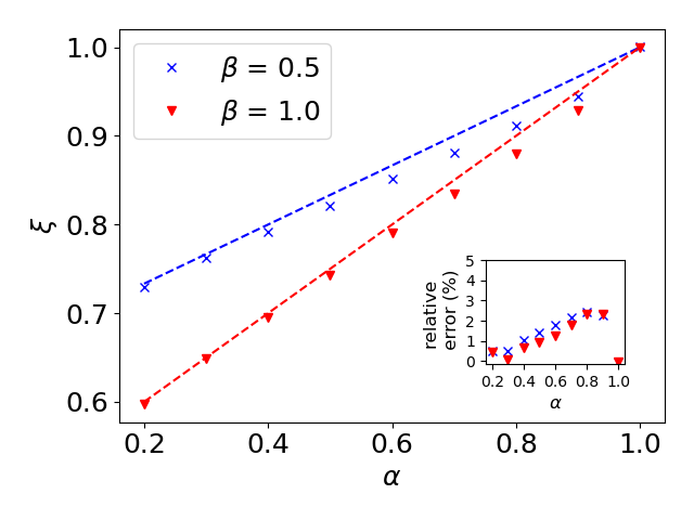
where $P_{\beta}(n,t)$ is the probability for a given $\beta$, see e.g., Eq. (Phase transition in non-Markovian animal exploration model with preferential returns). Although analytical progress is possible in the limit of $\sigma\!\ll\!1$ (SI, Sec. S1.D), Eq. (10) can generally be solved numerically (Fig. 1b). Notably, we checked that while variability in a population ($\sigma\!>\!0$) will not significantly affect the mean number of sites, it dramatically affects the variability across a population (SI, Fig. S2).

Statistics of number of visits to a site. Having computed the statistics of number of sites, we now turn to study the probability $W_{i}(m_{i},t)$ of having $m_{i}$ visits at time $t$ to an already visited site $i$, which follows

where $P_{new}$ and $\Pi_{i}$ are given by Eq. (1). In general, $\Pi_{i}$ depends on the number of visits to other sites, such that Eq. (Phase transition in non-Markovian animal exploration model with preferential returns) couples between different sites. Below, we focus on the limit $t\gg 1$, where $P_{new}\!\to\!0$ (SI, Sec. S2).

The case of $\alpha=1$. In the limit $t\gg 1$ we have $\sum_{i}m_{i}=t$, namely, the total number of visits to all sites equals the total number of time steps $t$. Thus, $\Pi_{i}(m_{i})=m_{i}/t$ and $P_{new}=0$ ³³3Here, Eq. (Phase transition in non-Markovian animal exploration model with preferential returns) is similar to the master equation in Ref. [22]. However, they only consider the case of $\beta=0$.. Equation (Phase transition in non-Markovian animal exploration model with preferential returns) is then solved by $W_{i}(m_{i},t)=t_{i}t^{-m_{i}}\left(t-t_{i}\right){}^{m_{i}-1},$ where $t_{i}$ is defined as the first time site $i$ is visited, $m_{i}(t=t_{i})=1$. The average is then $\left<m_{i}\right>=t/t_{i}$, while the variance $\sigma_{m_{i}}^{2}=\left<m_{i}^{2}\right>-\left<m_{i}\right>^{2}=t\left(t-t_{i}\right)/t_{i}^{2}\sim t^{2}$.

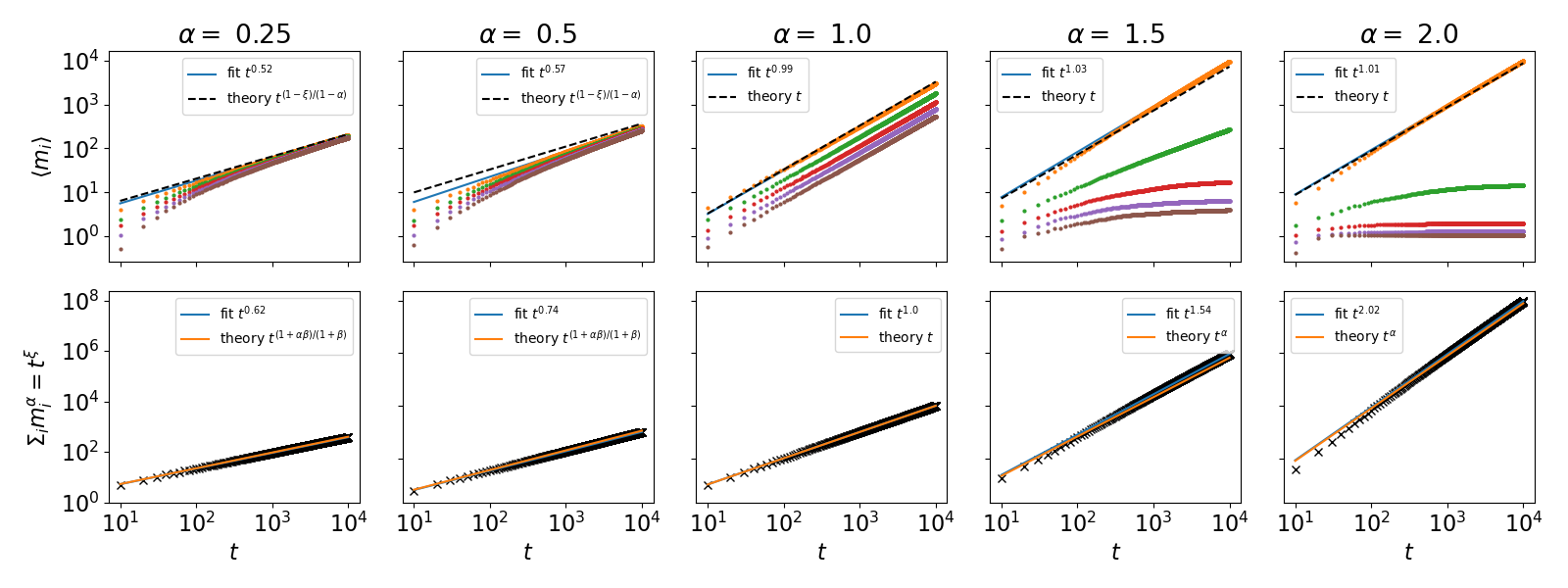
The case of $\alpha\neq 1$. Here, we a priori assume that $\sum_{j=1}^{\left<n\right>}\left<m_{j}\right>^{\alpha}\sim t^{\xi}$, where $\xi$ is a priori unknown and satisfies $\alpha<\xi<1$ (see SI, Sec. S2.A for proof). The average number of visits to any site $i$ can then be shown to asymptotically follow $\left<m_{i}\right>\sim t^{(1-\xi)/(1-\alpha)}[1+\mathcal{O}(t^{\xi-1})]$. Plugging this back into the sum over $\left<m_{j}\right>^{\alpha}$ we find that $\xi=\xi_{0}(1+\epsilon)$, where $\xi_{0}=(1+\alpha\beta)/(1+\beta)$ and $\epsilon\ll 1$ is an unknown function of $\alpha,\beta$ (Fig. S3). For $1-\alpha\ll\epsilon$ [$\beta=\mathcal{O}(1)$], we further find $\left<m_{i}\right>\sim t^{\beta/(1+\beta)}$, which is independent of $\alpha$; yet, the condition $1-\alpha\ll\epsilon$ breaks down as $\alpha$ approaches 1 (SI, Sec. S2.B and Fig. S4). Importantly, in the limit $t\gg 1$, for any $\alpha<1$ we find that all sites scale similarly with time. In contrast, for $\alpha>1$ not all site scale similarly with time. Here we find $\left<m_{i}\right>\simeq t$ for $i=1$, while $\left<m_{i}\right>\simeq C_{i}[1+\mathcal{O}(t^{1-\alpha})]$ for $i>1$, where $C_{i}=C_{i}(t_{i})$ is a constant (SI, Sec. S2.C).

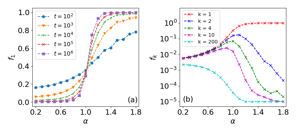
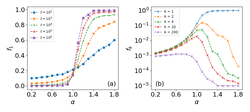
These results reveal a phase transition at $\alpha=1$ (see also SI, Sec. S2.D), where for weak PR ($\alpha<1$) the frequency of visits to the most visited site $f_{1}\equiv\left<m_{1}\right>/\sum_{j=1}^{\left<n\right>}\left<m_{j}\right>$ is only a small fraction of the total number of visits, while for strong PR ($\alpha>1$) $f_{1}$ approaches 1 as $t$ is increased and site 1 dominates (Fig. 2a). Importantly, in addition to the phase transition for $f_{1}$, the next most visited sites ($f_{k}$, for $k=2,3,...$) peak around $\alpha=1$ (Figs. 2b and S5). Here, as $\alpha$ approaches 0 the number of visits to all sites becomes similar, while for $\alpha>1$ these visitation frequencies tend to zero.

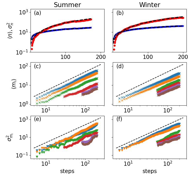
Movement of fruit bats. To study the relevance of our model for real-life systems and to obtain insights into the phase transition, we compare our predictions to resource use patterns and visitation dynamics of wild fruit bats tracked by ATLAS during winter and summer ⁴⁴4To have proper statistics and ensure no significant resource depletion, we analyse 10-day periods for each bat. For details on the species, seasonality and the segmentation and fitting procedures, see SI Sec. S3 and [4]. For details on ATLAS see [49, 11]. In Fig. 3a-b we fit the mean and variance of the number of visited sites (fruit trees) as a function of the number of movement steps (defined here as distinguishable movement between trees, see SI) to our theory ⁵⁵5 Note that the power-law dependence for the mean has also been experimentally observed in humans [21] and monkeys [25]; however, these studies did not analyze fluctuations around $\langle n\rangle$.. We find that during the summer $\beta_{0}$ and $\sigma$ are higher than during the winter, entailing lower rate of visits to new sites (higher levels of conformity) and larger inter-individual variability, respectively. Notably, many empirical studies have shown that individual preferences and decisions can affect movement and behavior, such that individuals do not have identical movement patterns [36, 37]. This may explain the inter-individual variability observed in both summer and winter. In Fig. 3c-f we show that during summer $\left<m_{1}\right>\sim t^{0.97}$ and $\left<m_{2}\right>\sim t^{0.99}$ (as well as $\sigma_{m_{1}}^{2}\sim t^{1.94}$ and $\sigma_{m_{2}}^{2}\sim t^{2.16}$), which matches the theory for $\alpha=1$. In contrast, during winter $\left<m_{1}\right>\sim t^{0.89}$ and $\left<m_{2}\right>\sim t^{0.87}$ ($\sigma_{m_{1}}^{2}\sim t^{1.96}$, $\sigma_{m_{2}}^{2}\sim t^{1.80}$), which is consistent with $\alpha$ values slightly below 1. These seasonal differences may be attributed to the fact that bats during the summer feed of highly abundant and palatable fruits – mulberries or figs with high levels of sugar content – and hence do not need to explore for feeding alternatives (high $\beta_{0}$) and can strongly rely on a limited number of sites ($\alpha=1$). Similarly, when food is abundant it makes sense that most bats will forage on the same bountiful locations, as they are not constrained by intense resource competition, thus reducing inter-individual variability in behaviour. In contrast, during winter there is less motivation to return to less favorable fruits (chinaberries) and a higher motivation to explore alternative trees, such as non-seasonal (unpredictable) fruit from the Ficus family.

In light of the phase transition at $\alpha=1$, and in agreement with experimental results, we hypothesize that in animal movement the value of $\alpha$ will tend towards 1. This maximizes the frequencies of visits to preferred sites (Fig. 2b), yet avoids an exclusive choice of a preferred site which occurs at $\alpha>1$ (see Fig. 2a). In this manner the animal combines intensive search patterns (committing to few site) with extensive searches (returning to all sites with some probability), a balance which is essential to optimize between energy expenditure and risk management [38, 39, 19]. Indeed, for fruit bats we find $\alpha\approx 1$, and similar results were obtained for humans [21] and monkeys [25]. Furthermore, the strategy of avoiding an exclusive site resembles bet-hedging strategies, e.g., bacterial persistence [40]. In addition, the value of $\alpha$ may be correlated to the total number of known sites: for large $\beta_{0}$ (few sites, summer) the bats will show stronger PR, while for smaller $\beta_{0}$ (more sites, winter) the strategy may tend towards a more uniform visitation rate to all trees.

More generally, we expect our results to also provide key insights into revisit dynamics in other areas like human mobility [41, 42, 43], COVID-19 spread [44], human migration [45] and languages dynamics [46].

Supplementary Information: Phase transition in non-Markovian animal exploration model with preferential returns

Here we provide additional details and results to support the derivations presented in the main text. Below, the notations and acronyms are the same as in the main text and the equations and figures refer to those therein.

References

- Nathan et al. [2008] R. Nathan, W. M. Getz, E. Revilla, M. Holyoak, R. Kadmon, D. Saltz, and P. E. Smouse, A movement ecology paradigm for unifying organismal movement research, Proceedings of the National Academy of Sciences 105, 19052 (2008).
- Grimm and Railsback [2005] V. Grimm and S. F. Railsback, Individual-based modeling and ecology, Vol. 8 (Princeton University Press, 2005).
- Metzler et al. [2014] R. Metzler, J.-H. Jeon, A. G. Cherstvy, and E. Barkai, Anomalous diffusion models and their properties: non-stationarity, non-ergodicity, and ageing at the centenary of single particle tracking, Physical Chemistry Chemical Physics 16, 24128 (2014).
- Lourie et al. [2021] E. Lourie, I. Schiffner, S. Toledo, and R. Nathan, Memory and conformity, but not competition, explain spatial partitioning between two neighboring fruit bat colonies, Frontiers in Ecology and Evolution , 711 (2021).
- Gurarie et al. [2016] E. Gurarie, C. Bracis, M. Delgado, T. D. Meckley, I. Kojola, and C. M. Wagner, What is the animal doing? tools for exploring behavioural structure in animal movements, Journal of Animal Ecology 85, 69 (2016).
- Fagan et al. [2013] W. F. Fagan, M. A. Lewis, M. Auger-Méthé, T. Avgar, S. Benhamou, G. Breed, L. LaDage, U. E. Schlägel, W.-w. Tang, Y. P. Papastamatiou, et al., Spatial memory and animal movement, Ecology letters 16, 1316 (2013).
- Bracis et al. [2015] C. Bracis, E. Gurarie, B. V. Moorter, and R. A. Goodwin, Memory effects on movement behavior in animal foraging, PLOS ONE 10, e0136057 (2015).
- Polansky et al. [2015] L. Polansky, W. Kilian, and G. Wittemyer, Elucidating the significance of spatial memory on movement decisions by african savannah elephants using state–space models, Proceedings of the Royal Society B: Biological Sciences 282, 20143042 (2015).
- Ranc et al. [2021] N. Ranc, P. R. Moorcroft, F. Ossi, and F. Cagnacci, Experimental evidence of memory-based foraging decisions in a large wild mammal, Proceedings of the National Academy of Sciences 118 (2021).
- Goldshtein et al. [2020] A. Goldshtein, M. Handel, O. Eitan, A. Bonstein, T. Shaler, S. Collet, S. Greif, R. A. Medellín, Y. Emek, A. Korman, et al., Reinforcement learning enables resource partitioning in foraging bats, Current Biology 30, 4096 (2020).
- Toledo et al. [2020] S. Toledo, D. Shohami, I. Schiffner, E. Lourie, Y. Orchan, Y. Bartan, and R. Nathan, Cognitive map–based navigation in wild bats revealed by a new high-throughput tracking system, Science 369, 188 (2020).
- Krochmal et al. [2021] A. R. Krochmal, T. C. Roth, and N. T. Simmons, My way is the highway: the role of plasticity in learning complex migration routes, Animal Behaviour 174, 161 (2021).
- Morales et al. [2004] J. M. Morales, D. T. Haydon, J. Frair, K. E. Holsinger, and J. M. Fryxell, Extracting more out of relocation data: building movement models as mixtures of random walks, Ecology 85, 2436 (2004).
- Patterson et al. [2008] T. Patterson, L. Thomas, C. Wilcox, O. Ovaskainen, and J. Matthiopoulos, State-space models of individual animal movement, Trends in Ecology & Evolution 23, 87 (2008).
- Riotte-Lambert et al. [2015] L. Riotte-Lambert, S. Benhamou, and S. Chamaillé-Jammes, How memory-based movement leads to nonterritorial spatial segregation, The American Naturalist 185, E103 (2015).
- Hod and Keshet [2004] S. Hod and U. Keshet, Phase transition in random walks with long-range correlations, Physical Review E 70, 015104 (2004).
- Schütz and Trimper [2004] G. M. Schütz and S. Trimper, Elephants can always remember: Exact long-range memory effects in a non-markovian random walk, Physical Review E 70, 045101 (2004).
- Evans and Majumdar [2011] M. R. Evans and S. N. Majumdar, Diffusion with stochastic resetting, Physical Review Letters 106, 160601 (2011).
- Berger-Tal and Bar-David [2015] O. Berger-Tal and S. Bar-David, Recursive movement patterns: review and synthesis across species, Ecosphere 6, 1 (2015).
- Evans et al. [2020] M. R. Evans, S. N. Majumdar, and G. Schehr, Stochastic resetting and applications, Journal of Physics A: Mathematical and Theoretical 53, 193001 (2020).
- Song et al. [2010] C. Song, T. Koren, P. Wang, and A.-L. Barabási, Modelling the scaling properties of human mobility, Nature Physics 6, 818 (2010).
- Boyer and Solis-Salas [2014] D. Boyer and C. Solis-Salas, Random walks with preferential relocations to places visited in the past and their application to biology, Physical Review Letters 112, 240601 (2014).
- Boyer and Romo-Cruz [2014] D. Boyer and J. C. R. Romo-Cruz, Solvable random-walk model with memory and its relations with markovian models of anomalous diffusion, Physical Review E 90, 042136 (2014).
- Campos and Méndez [2019] D. Campos and V. Méndez, Recurrence time correlations in random walks with preferential relocation to visited places, Physical Review E 99, 062137 (2019).
- Boyer et al. [2012] D. Boyer, M. C. Crofoot, and P. D. Walsh, Non-random walks in monkeys and humans, Journal of The Royal Society Interface 9, 842 (2012).
- Krapivsky et al. [2000] P. L. Krapivsky, S. Redner, and F. Leyvraz, Connectivity of growing random networks, Physical review letters 85, 4629 (2000).
- Note [1] Similar growth rates appear in self-inhibitory gene regulatory networks, where a protein inhibits its own growth, see e.g., Refs. [47, 48].
- Note [2] In the SI, Sec. S1.B we alternatively develop a a generating function approach, and Eq. (2\@@italiccorr) becomes a fractional integro-differential equation, which is solvable in specific cases.
- Assaf and Meerson [2006] M. Assaf and B. Meerson, Spectral formulation and wkb approximation for rare-event statistics in reaction systems, Physical Review E 74, 041115 (2006).
- Dykman et al. [1994] M. I. Dykman, E. Mori, J. Ross, and P. Hunt, Large fluctuations and optimal paths in chemical kinetics, The Journal of chemical physics 100, 5735 (1994).
- Elgart and Kamenev [2004] V. Elgart and A. Kamenev, Rare event statistics in reaction-diffusion systems, Physical Review E 70, 041106 (2004).
- Assaf and Meerson [2017] M. Assaf and B. Meerson, Wkb theory of large deviations in stochastic populations, Journal of Physics A: Mathematical and Theoretical 50, 263001 (2017).
- Note [3] Here, Eq. (Phase transition in non-Markovian animal exploration model with preferential returns\@@italiccorr) is similar to the master equation in Ref. [22]. However, they only consider the case of .
- Note [4] To have proper statistics and ensure no significant resource depletion, we analyse 10-day periods for each bat. For details on the species, seasonality and the segmentation and fitting procedures, see SI Sec. S3 and [4]. For details on ATLAS see [49, 11].
- Note [5] Note that the power-law dependence for the mean has also been experimentally observed in humans [21] and monkeys [25]; however, these studies did not analyze fluctuations around .
- Dingemanse et al. [2002] N. J. Dingemanse, C. Both, P. J. Drent, K. Van Oers, and A. J. Van Noordwijk, Repeatability and heritability of exploratory behaviour in great tits from the wild, Animal Behaviour 64, 929 (2002).
- Dingemanse and Dochtermann [2013] N. J. Dingemanse and N. A. Dochtermann, Quantifying individual variation in behaviour: mixed-effect modelling approaches, Journal of Animal Ecology 82, 39 (2013).
- Bartumeus et al. [2014] F. Bartumeus, E. P. Raposo, G. M. Viswanathan, and M. G. E. da Luz, Stochastic optimal foraging: Tuning intensive and extensive dynamics in random searches, PloS ONE 9 (2014).
- Nolting et al. [2015] B. C. Nolting, T. M. Hinkelman, C. E. Brassil, and B. Tenhumberg, Composite random search strategies based on non-directional sensory cues, Ecological Complexity 22, 126 (2015).
- Balaban et al. [2004] N. Q. Balaban, J. Merrin, R. Chait, L. Kowalik, and S. Leibler, Bacterial persistence as a phenotypic switch, Science 305, 1622 (2004).
- Schlosser and Brockmann [2021] F. Schlosser and D. Brockmann, Finding disease outbreak locations from human mobility data, EPJ data science 10, 52 (2021).
- do Couto Teixeira et al. [2021] D. do Couto Teixeira, J. M. Almeida, and A. C. Viana, On estimating the predictability of human mobility: the role of routine, EPJ Data Science 10, 49 (2021).
- Schläpfer et al. [2021] M. Schläpfer, L. Dong, K. O’Keeffe, P. Santi, M. Szell, H. Salat, S. Anklesaria, M. Vazifeh, C. Ratti, and G. B. West, The universal visitation law of human mobility, Nature 593, 522 (2021).
- Galeazzi et al. [2021] A. Galeazzi, M. Cinelli, G. Bonaccorsi, F. Pierri, A. L. Schmidt, A. Scala, F. Pammolli, and W. Quattrociocchi, Human mobility in response to covid-19 in France, Italy and UK, Scientific Reports 11, 1 (2021).
- Chi et al. [2020] G. Chi, F. Lin, G. Chi, and J. Blumenstock, A general approach to detecting migration events in digital trace data, PloS ONE 15, e0239408 (2020).
- Watanabe [2018] H. Watanabe, Empirical observations of ultraslow diffusion driven by the fractional dynamics in languages, Physical Review E 98 (2018).
- Dublanche et al. [2006] Y. Dublanche, K. Michalodimitrakis, N. Kümmerer, M. Foglierini, and L. Serrano, Noise in transcription negative feedback loops: simulation and experimental analysis, Molecular Systems Biology 2, 41 (2006).
- Roberts et al. [2015] E. Roberts, S. Be’er, C. Bohrer, R. Sharma, and M. Assaf, Dynamics of simple gene-network motifs subject to extrinsic fluctuations, Physical Review E 92, 062717 (2015).
- Weiser et al. [2016] A. W. Weiser, Y. Orchan, R. Nathan, M. Charter, A. J. Weiss, and S. Toledo, Characterizing the accuracy of a self-synchronized reverse-gps wildlife localization system, in 2016 15th ACM/IEEE International Conference on Information Processing in Sensor Networks (IPSN) (IEEE, 2016) pp. 1–12.
- Abramowitz and Stegun [1964] M. Abramowitz and I. A. Stegun, Handbook of Mathematical Functions with Formulas, Graphs, and Mathematical Tables, ninth dover printing, tenth gpo printing ed. (Dover, New York, 1964).
- Gardiner [2009] C. Gardiner, Stochastic methods, Vol. 4 (Springer Berlin, 2009).
- Arfken and Weber [1999] G. B. Arfken and H. J. Weber, Mathematical methods for physicists (1999).
- Kwiecinski and Griffiths [1999] G. G. Kwiecinski and T. A. Griffiths, Rousettus egyptiacus, Mammalian Species , 1 (1999).
- Egert-Berg et al. [2018] K. Egert-Berg, E. R. Hurme, S. Greif, A. Goldstein, L. Harten, J. J. Flores-Martínez, A. T. Valdés, D. S. Johnston, O. Eitan, I. Borissov, et al., Resource ephemerality drives social foraging in bats, Current Biology 28, 3667 (2018).
- Gupte et al. [2020] P. R. Gupte, C. E. Beardsworth, O. Spiegel, E. Lourie, S. Toledo, R. Nathan, and A. I. Bijleveld, A guide to pre-processing high-throughput animal tracking data, bioRxiv (2020).