Phase transition patterns for coupled complex scalar fields at finite temperature and density
Abstract
The phase transition patterns displayed by a model of two coupled complex scalar fields are studied at finite temperature and chemical potential. Possible phenomena like symmetry persistence and inverse symmetry breaking at high temperatures are analyzed. The effect of finite density is also considered and studied in combination with the thermal effects. The nonperturbative optimized perturbation theory method is considered and the results contrasted with perturbation theory. Applications of the results obtained are considered in the context of an effective model for condensation of kaons at high densities, which is of importance in the understanding of the color-flavor locked phase of quantum chromodynamics.
I Introduction
In statistical physics, we can describe a dynamical system in the ensemble as characterized by a Hamiltonian, with charges (or quantum numbers) and corresponding chemical potentials. A chemical potential, which enters as a Lagrange multiplier in the (quantum) grand-canonical partition function, is assigned to each conserved charge of the system. This is the starting point of any setup aiming to study how a conserved charge (or conserved charges) eventually affects the phase structure of the system, e.g., in the Bose-Einstein condensation problem huang .
The study of how a finite charge can affect the phase transition for a scalar field in the context of quantum field theory dates back for example from the pioneering works of Kapusta Kapusta:1981aa , Haber and Weldon Haber:1981fg ; Haber:1981ts among others. In Refs. Bernstein:1990kf ; Benson:1991nj it was observed that finite charges can modify strongly the phase transition structure of a complex scalar field. In particular, it was shown in details in Ref.Benson:1991nj that a sufficiently large fixed charge in the context of a constant ratio for the number over entropy densities, like for instance as expected to appear in cosmological settings, a broken symmetry could persist at sufficiently high temperatures. Likewise, under the same conditions, an originally symmetric phase in the vacuum could get broken at high temperatures. This is what characterizes a symmetry inversion phase transition at high temperatures. These type of phenomena are reminiscent of a symmetry nonrestoration (SNR) or inverse symmetry breaking (ISB) type of transitions first studied by Weinberg in Ref. Weinberg:1974hy . The difference here, it is that these unusual transition patterns studied in Ref. Benson:1991nj would originate from finite density effects already in the case of an one field case, whereas in Ref. Weinberg:1974hy they originate only at finite temperatures for the case of multiple coupled scalar fields, with both inter and intracouplings and with suitable choices of those coupling constants.
In the present paper, we reanalyze the effects of finite density in the phase structure of complex scalar fields, but accounting for both situations that were studied in Ref. Weinberg:1974hy and in Ref. Benson:1991nj . Here, we are then interested in the case where the interplay of both coupling constants, thermal effects and finite charges can compete or complement each other in the way they can affect in unusual ways the phase structure of the system. While the finite charges effects in the phase structure of a complex scalar field were originally studied in the context of the perturbative high temperature approximation in Ref. Benson:1991nj , here we also want to reevaluate that in terms of the nonperturbative method of the optimized perturbation theory (OPT) Stevenson:1981vj ; Okopinska:1987hp ; Klimenko:1992av ; Kleinert:1998zz ; Chiku:1998kd ; Pinto:1999py ; Pinto:1999pg ; Farias:2008fs (see also, e.g., Ref. Yukalov:2019nhu for a recent review). This is specially important since perturbation theory studies of phase transitions at high temperatures may be unreliable as it is well known, which motivates the use of different nonperturbative methods (see, e.g., Refs. Curtin:2016urg ; Croon:2020cgk ; Senaha:2020mop ; Schicho:2021gca ; Gould:2021oba for reviews and recent discussions).
At the final part of this work and as an applications of our results, we will consider the condensation of kaons in the color-flavor locked (CFL) phase of quantum chromodynamics (QCD). The CFL phase is a color-superconducting phase where diquark condensates break the chiral symmetry Alford:1998mk (for a review, see, e.g., Ref. Alford:2007xm ). The symmetry breaking pattern of this phase transition can be associated with light pseudo-Nambu Goldstone bosons, where the lightest of them are the charged and neutral kaons. The study of the condensation of these light kaons has been shown to be possible to be described in terms of an -symmetric effective scalar field theory Alford:2007qa ; Andersen:2008tn ; Tran:2008mvg that turns out to be analogous to the coupled two complex scalal field we study in the present paper. In the previous works Alford:2007qa ; Andersen:2008tn ; Tran:2008mvg the CFL phase related to kaons condensation were studied in the Cornwall-Jackiw-Tomboulis (CJT) nonperturbative method Cornwall:1974vz ; Amelino-Camelia:1992qfe . The use of the OPT method here allows us not only to compare with those earlier results obtained with the CJT method, but also allows us to discuss the Goldstone theorem, which was shown to be problematic in those studies. However, in the OPT case, the Goldstone theorem is exactly satisfied as we will show.
The remainder of this paper is organized as follows. In Sec. II, we introduce the model studied in this paper, along also with its implementation in the context of the OPT method. The relevant thermodynamic quantities for our study are also derived. In Sec. III, we give the many numerical results exploring both ISB and SNR realizations in the model and the many possibilities of phase transition patterns that can emerge at finite chemical potential and charge densities in a thermal environment. In Sec. IV, we apply our results for the case of an effective model derived from a chiral Lagrangian density describing the condensation of kaons in a CFL phase for QCD at high densities. Our conclusions are presented in Sec. V. Two appendices are also included, where some of the technical details are presented.
II OPT implementation for the two complex scalar field model
We consider a model with two complex scalar fields, and , with quartic self-interactions and a biquadratic intercoupling between them. The Lagrangian density is given by
| (1) | |||||
It is convenient to write the complex scalar fields and in terms of their real and imaginary components as, and . The Lagrangian density (1) then becomes
| (2) | |||||
where the tree-level potential is
| (3) | |||||
The stability of the potential requires , and, when , that . The intercoupling , hence, can be either positive or negative. We will be particularly interested in the case where can assume negative values.
II.1 The effective potential at finite temperature and chemical potential
The thermodynamical potential density is defined as
| (4) |
where is the space volume and is the grand partition function,
| (5) |
where , is the Hamiltonian operator, denotes the conserved charge operators and are the corresponding chemical potentials. The grand partition function can be written as a functional integral over the fields as usual in quantum field theory Kapusta:2006pm . In the integral functional field form, the grand partition function for the model Eq. (1) then becomes
| (6) |
where the functional integrals over the fields are performed under the periodic boundary conditions in imaginary Euclidean time, and , and the Euclidean action is given by
| (7) | |||||
The expression (6) with Eq. (7) generalizes for the present case of a system with two complex coupled scalar fields the one obtained in the case of one only complex scalar field case, as given, e.g., in Ref. Kapusta:2006pm (see also Ref. Benson:1991nj ).
II.2 The OPT implementation
The general implementation of the OPT in the Lagrangian density happens through an interpolation defined as (see, e.g., Refs. Rosa:2016czs ; Farias:2021ult and references there in)
| (8) |
where is the Lagrangian density of the free theory, which is modified by an arbitrary mass parameter .
The standard interpolation procedure given by Eq. (8) gives for our model the following Lagrangian density
| (9) | |||||
with , , where are mass parameters determined through a variational procedure (see below) and is a dimensionless parameter used as a bookkeeping parameter only to keep track of the order that the OPT is implemented and is set to one at the end. Note that the OPT interpolation changes the usual Feynman rules of the theory. The quartic vertices are changed to
| (10) |
and the OPT also leads to the additional vertices that come from the interpolation procedure and that are quadratic in the fields, which comes from the last two terms appearing in Eq. (9). Their Feynman rules are simply
| (11) |
while the bare propagators for the fields have masses replaced in the OPT procedure by and .
All calculations are carried out similarly as done in perturbation theory and can be evaluated at any order in . Hence, up to this stage the results remain strictly perturbative and very similar to the ones obtained via an ordinary perturbative calculation. Since all quantities evaluated at any finite order in the OPT depends explicitly on , these parameters need to be fixed appropriately. It is through the freedom in fixing that nonperturbative results can be generated in the OPT. Since do not belong to the original theory, these parameters need to be fixed considering some appropriate procedure. For instance, one may fix them by requiring that a given physical quantity, which is been calculated perturbatively to order-, to be evaluated at the value where it is less sensitive to this parameter. This criterion is known as the principle of minimal sensitivity (PMS) Stevenson:1981vj . In this work we consider the effective thermodynamic potential (ETP), which is evaluated to order-, , as the appropriate quantity to be optimized and as considered in most of the OPT works in general111See, for example, Refs. Farias:2008fs ; Rosa:2016czs ; Yukalov:2019nhu , for examples of other different quantities that can be optimized, different optimization methods and a comparison between the results.. In this case, the PMS criterion translates into the variational relation
| (12) |
There can also be other optimization procedures that can be applied to fix the OPT mass parameters, but they have shown to be equivalent to the PMS one, including the convergence properties (see, see for instance, Ref. Rosa:2016czs for a discussion on these issues). The optimum value for and derived from Eq. (12) are now nontrivial functions of the original parameters of the theory. In particular, and become explicit functions of the couplings and, as a consequence of this, nonperturbative results are generated.
II.3 The ETP in the OPT approximation

By shifting the fields around their respective background expectations values in Eq. (9), which can be taken along and without loss of generality, then and , with and and , we can, thus, derive the effective potential at first order in the OPT, i.e., at first order in . All terms contributing to the ETP to first order in the OPT are given in Fig. 1. They are all explicitly derived in the Appendix A and the renormalized ETP at first order in the OPT is then given by
| (13) | |||||
where the functions and haven been defined in the Appendix A and given by Eqs.(45) and (46), respectively.
II.4 Optimization procedure
Applying the PMS procedure Eq. (12) to the renormalized ETP Eq. (13), we obtain that and are obtained from the coupled equations,
which are to be solved together with the ones defining the background field values and , obtained from,
| (16) |
which give, respectively, the expressions,
| (17) | |||
| (18) |
Equations (17) and (18) have the trivial solutions, , while the coupled gap equations valid when and are given, respectively, by
| (19) | |||
| (20) |
Note that by combining Eqs. (LABEL:pmsetaphi) and (LABEL:pmsetapsi) with Eqs. (19) and (20), we obtain
| (21) |
and
| (22) |
which gives that at the critical point for, e.g., in the -direction, , the critical chemical potential gets uniquely fixed by
| (23) |
and, equivalently, at the critical point in the -direction, , it leads to
| (24) |
Equations (23) and (24) generalize to the present problem the usual condition for Bose-Einstein condensation (BEC) for an ideal Bose gas Kapusta:2006pm , at the critical temperature for BEC. Note that the contribution from the interactions to the BEC transition point enters implicitly in the OPT functions, and , in Eqs. (23) and (24).
II.5 The densities
From the effective thermodynamical potential, we can compute the pressure,
| (25) |
which is evaluated at the PMS values and and at the VEV values and . Given the pressure, the densities are evaluated as
| (26) | |||
| (27) |
Then, making use of Eq. (13) in combination with the PMS equation (12), we find
| (28) | |||||
| (29) |
Note that the above equations for and are to be solved simultaneously with those for the PMS, Eqs. (LABEL:pmsetaphi)and (LABEL:pmsetapsi), together with those for the background fields, Eqs. (17) and (18).
III ISB and SNR in a thermal and dense medium: results
When the square masses and are both positive in the tree-level potential Eq. (3) and under appropriate choice of coupling constants satisfying the boundness condition for the potential, we have the possibility of having ISB in one of the directions at high temperatures, while the other field remains in the symmetric phase. On the other hand, when the square masses and are both negative in the tree-level potential Eq. (3), we have the possibility of having SNR for one of the fields at high temperatures, while the other one will suffer the usual symmetry restoration at some critical temperature .
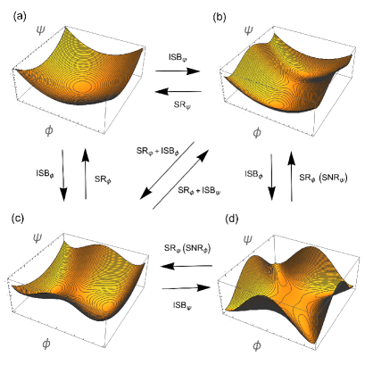
Figure 2 illustrates the different phases in which the system might display depending on the choices made for the model parameters, temperature and density. Let us describe the four cases illustrated in Fig. 2. Case (a): the system is in the symmetric state with respect to the two fields, . Case (b): the system is in a state with symmetry breaking in the direction of , , and symmetry restored in the direction of , . Case (c): the system is in a state with symmetry breaking in the direction of , , and symmetry restored in the direction of , . Case (d): the system is in the symmetry broken state with respect to the two fields, and . The arrows indicate the possible transitions that the system might experience when changing and/or and .
In the results below, we will analyze these different cases. We will first analyze the situation where ISB becomes possible at high temperatures, and then the situation where SNR becomes viable. For convenience and without loss of generality, we will assume and . All quantities are normalized by the regularization scale .
III.1 The ISB case: and
For our numerical results we will consider for illustration purposes the base parameters values for the couplings: , and . Note that though , we have that , thus, this choice of couplings satisfies the boundness condition for the potential. In other words, the tree potential is safely inside the stable region. Other choices can be made but the results are qualitatively similar under the conditions considered here. Thus, by considering and the set of coupling parameters given above, ISB can be shown to happen in the direction of at high temperatures, while remains in the symmetric phase. This is what simple perturbation theory at high temperatures would predict for the two-field coupled complex scalar model in the absence of chemical potentials Farias:2021ult . Note that we can recover the PT results from the OPT interpolated ETP Eq. (13) by setting , which then gives the ETP at first order in the coupling constants in the first order PT approximation. In the OPT case, we do obtain though, quantitative differences when compared with the results from PT as we are going to illustrate.
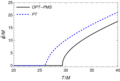
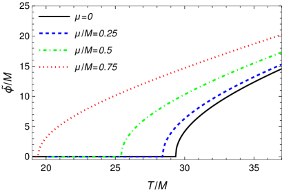
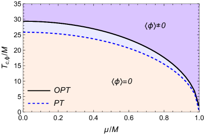
The situation illustrated in the Fig. 3 demonstrates ISB in the direction of the field . Starting from a symmetry restored (SR) state at , the field eventually acquires a nonvanishing VEV at a critical temperature. Both OPT and PT are compared. One notices that the OPT tends to produce a higher critical temperature than in the PT approximation case. Given the parameters considered, the field remains in the SR phase. The effect of a finite chemical potential on the behavior for the VEV of the field is illustrated in the Fig. 4. Note that for our choice of parameters and for held constant at the values considered, the field remains always with a vanishing background expectation value, , hence, we do not show it in Figs. 3 and 4. In Fig. 4, we restrict only to show the OPT case, since for PT the results are similar, with the same trend as seen in Fig. 3, leading to smaller critical temperatures when compared to the OPT. From the results shown in Fig. 4, we see that the chemical potential tends to decrease the critical temperature for ISB. Thus, the larger is the chemical potential, the easier is to reach symmetry inversion in the direction of , i.e., the field acquires a VEV at lower temperatures as the chemical potential increases. As the field changes smoothly through the critical point, the phase transition associated with ISB here is of second order. The overall behavior for the critical temperature for ISB in the direction of , , as a function of the chemical potential, is shown in Fig. 5.
The Fig. 5 shows that the higher the chemical potential, the lower the value of the critical temperature. The presence of charge is seen here to favor symmetry inversion (ISB), causing it to happen at a lower critical temperature.
From the mass eigenvalues expressions given in Appendix B, we can define the corresponding Higgs and Goldstone effective modes for and in the context of the OPT. This can be done by introducing in the definitions Eq. (81), the thermal and chemical potential contributions such that Duarte:2011ph ; Farias:2021ult , , and similarly for the field, where, at first order in the OPT,
| (30) | |||||
| (31) | |||||
| (32) | |||||
| (33) | |||||
where and are obtained from the solution of Eq. (16), while and from the PMS equations (LABEL:pmsetaphi) and (LABEL:pmsetapsi). Note that the Higgs modes must remain positive in both symmetric and broken phases, while vanishing at the critical point for phase transition. The Goldstone modes, on the other hand, must remain massless in the broken phases, according to the Goldstone theorem concerning symmetry breaking of a continuous symmetry, while in the symmetric phase follows the Higgs modes.
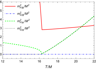
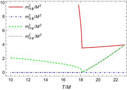
Substituting Eqs. (30)-(33) in the mass eigenvalue equation (82)-(85), we obtain the corresponding ones at finite temperature and chemical potential, . These Higgs and Goldstone modes for each of the fields are plotted in Fig. 6 for the cases of vanishing chemical potentials (panel a) and also for nonvanishing chemical potential (panel b). In both cases we see that the Goldstone theorem is correctly reproduced. The fact that the OPT satisfies the Goldstone theorem has also been seen in previous applications Duarte:2011ph ; Farias:2021ult .
III.2 The SNR case: and
In the previous subsection, we have investigated the two coupled complex scalar field at finite temperature and chemical potential with respect to symmetry inversion (ISB). Let us now study the model for symmetry persistence at high temperatures, i.e., we will study the case for SNR in one of the field directions. We continue to use the same set of bare coupling constants as before for clarity, but now we consider that the symmetries for both the fields, in the vacuum, are both broken, and , such that both fields have a nonvanishing VEV at and initially. In this case, we expect SNR in the direction of , while should suffer the usual symmetry restoration (SR) at high temperatures. This is illustrated in Fig. 7.
In Fig. 8 we show the Higgs and Goldstone modes for the fields when (panel a) and when (panel b) for the present case of SNR in the direction of and SR in the direction of . As in the case studied in the previous subsection, we also see here that the Goldstone theorem is correctly reproduced.
III.3 OPT results at finite temperature and density
Let us now turn our attention of how a finite density affects the results. In the previous two subsections we were interested in the effect of a finite chemical potential in the transition patterns displayed by the two coupled complex scalar field system. Here, we are interested in investigating the same effects but now at finite densities. This is mostly motivated by the seminal work performed in Refs. Bernstein:1990kf ; Benson:1991nj . In particular, in Ref. Benson:1991nj it was shown that finite density effects were already able to not only delay symmetry restoration at finite temperature, but also to promote symmetry nonrestoration for a sufficiently large charge (density). The novelty result was that both ISB and SNR could be possible already for a one-field model case. Here, we are interested in studying how the finite density effects will further affect the phase transition pattern when considering the case of more than one coupled complex scalar field. In order to facilitate the comparison with Ref. Benson:1991nj , we will also assume densities for the fields such that the ratio of number density to entropy density is kept fixed. The motivation here, as also in Ref. Benson:1991nj , stems from the fact that in an adiabatic expansion, with the entropy remaining constant, the ratio of charge density over entropy density remains constant. This is like the expected situation in the case of the expanding Universe in the radiation dominated phase when in the absence of entropy production processes. Thus, we assume from now on that the charge density of the fields over entropy energy density remains constant, . Since in the ultrarelativistic case, and , we take Benson:1991nj
| (34) |
where is the proportionality constant222Note that in Ref. Benson:1991nj the proportionality constant was denoted by . To not confuse with the OPT usual parameter notation, we use here instead as the proportionality constant. . For simplicity, we will also assume . The case of asymmetries in the charge densities can be implemented without difficult, which can be of interest in the case of systems with large differences in the parameters (e.g., in the masses, or which can have large differences in the way both fields might be coupled to additional radiation fields in the system).
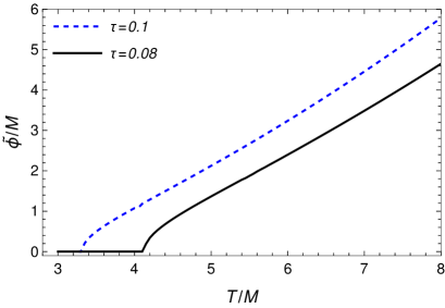
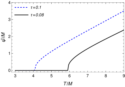
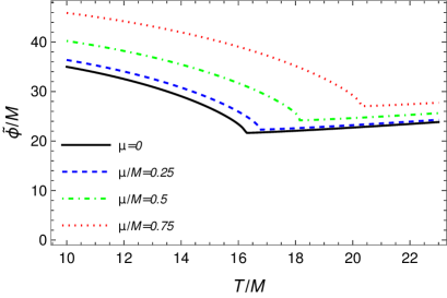
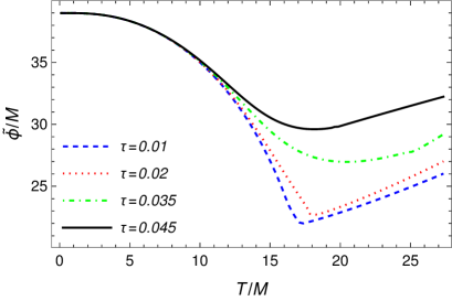
By using Eq. (34) in conjunction with the equations defining the densities, Eqs. (28) and (29), together with the PMS and gap equations, we study the behavior of the fields expectations values and as a function of the temperature and fixed ratio . In Fig. 9 it is shown the VEV of the fields, (panel a) and (panel b), as a function of temperature. Two representative values of have been used for illustration. Note that for the parameters considered, in the absence of finite charge effects ISB is expected to happen in the direction of the field (see, e.g., Fig. 3). In the presence of finite charge densities, we see that two effects appear. First, the ISB transition can happen earlier, i.e., at a lower critical temperature. Second, there is now also an ISB transition in the field direction, i.e., can now acquire a nonvanishing value at finite temperatures and also here we see that the larger is , the lower is the critical temperature for ISB in the direction of . Finite charges are then realizing the transition pattern (a) (b) (d) shown in Fig. 1 in the present case.
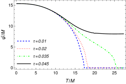
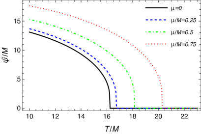
In Fig. 10 we now consider the case where both fields are initially in their broken symmetry states, i.e., and at and . For the parameters considered, in the absence of finite charge densities, the transition pattern expected is the one shown in Fig. 7, i.e., SNR in the direction of and usual SR transition in the direction of . From Fig. 10 we now see that besides the field remaining in a SNR state, now the finite charge density also induces a SNR in the direction of the field. For the parameters considered in Fig. 10, for a charge density over entropy density ratio , we find that it ceases to exist a critical temperature for SR in the direction of and the field remains in a SNR state.
As a note to be remarked here, even though we have in this part of the work continued to work with a negative value for the intercoupling , in the presence of finite charge densities both situations shown in Figs. 9 and 10 are still realized. ISB and SNR happens independently of the sign of the coupling between and . This happens exclusively because of the effect of considering large enough densities. Our results then generalize to the two-field case the situation found in Ref. Benson:1991nj , where it was studied for the one-field case.
IV Application to condensations of kaons
As one of the possible applications of the methods and results studied in this paper, one can consider the problem of the condensation of kaons in QCD. Let us start by briefly reviewing the role of kaons in the so-called CFL phase of QCD at high densities and how it can be modeled with a system analogous to the model we have studied in the previous sections.
In QCD with three degenerate flavors and at asymptotically high density and low temperatures, the ground state for the quark matter is supposed to be in the so-called CFL state Alford:1998mk ; Alford:2007xm , with diquark condensates. This is a color superconducting state, where the quarks can pair and form Cooper pairs, similar to what happens to electrons in a condensed matter superconductor material. In this situation, that can happen at sufficiently large densities, the original symmetry group , with the color gauge group and the chiral symmetry group , is broken down to . The residual group locks the rotations of color with rotations of the flavor, since is a linear combination of the generators of the original group. The breakdown of the chiral symmetry gives origin to an octet of pseudo-Goldstone modes and a singlet mode, which comes from the breakdown of the baryon-number group . The latter group is called the superfluid mode, since it is responsible for the superfluidity of the CFL phase. At high densities all of the modes can be regarded as approximately massless by neglecting the masses of the quarks (e.g., the quarks up, down and strange). This is a rather different situation than that one at moderated densities, when the chiral symmetry is explicitly broken and the superfluid mode is the only one that remains massless, while the meson modes acquire mass. This scenario, of moderate densities (about the order of several times the nuclear density), is the one expected for example in the interior of neutron stars Lee:1996ef and the order of the expected value for the chemical potential is about MeV. The lightest mesons, except the massless superfluid mode, are the charged and neutral kaons , and , , while the strange quark, for example, has its mass in somewhere between the current quark mass, MeV and the constituent quark mass, MeV. Likewise, it is to be noted that for a boson chemical potential larger than its vacuum mass, the boson will suffer a Bose condensation. This is what is supposed to happen with kaons in a dense medium. The low in-medium kaon mass can, thus, lead to the formation of a kaon condensate.
As the symmetry-breaking pattern explained above is the same as in vacuum QCD, it is expected the low-energy properties of the CFL phase to be well described in terms of an effective chiral Lagrangian at high densities for the octet of (pseudo-) Goldstone modes and the superfluid mode. The condensation of kaons can then be described by an effective chiral Lagrangian density for the mesons in the CFL phase as given by Alford:2007qa ; Andersen:2008tn
where denotes the meson field, are the Gell-Mann matrices, , , and are constants, which can be found by appropriate matchings Son:1999cm ; Kaplan:2001qk ; Schafer:2002ty . In Eq. (LABEL:chiralL) is the chemical potential for electric charge and describes the octet of Goldstone bosons. The ellipses in Eq. (LABEL:chiralL) stand for higher order terms in the chiral Lagrangian density expansion. The matrix acts as a zeroth component of a gauge field, which can be expressed in terms of the diagonal matrices and , with the chemical potential and the baryon chemical potential related by .
Using perturbative calculations for QCD at high densities, it is possible to determine the parameters , and . By writing the meson field as
| (36) |
and expanding to fourth order in the meson fields, from the Lagrangian density (LABEL:chiralL), the effective Euclidean Lagrangian density for the kaons can be written in the form Alford:2007qa
| (37) | |||||
where the complex doublet scalar field can be identified with the charged and the neutral kaons, , with the chemical potentials and associated with the conserved charges for and , respectively. The effective model for the kaons, when expressed in the form of Eq. (37), is just of the same form as the model we have studied here, in terms of the Euclidean action Eq. (7), and by identifying, e.g., with , or, equivalently, with , with also , , , and .
In Refs. Alford:2007qa ; Andersen:2008tn ; Tran:2008mvg the kaon condensation problem with the effective model Eq. (37) was studied using the CJT method. Here, we want to compare the same results but in terms of the OPT. This also gives us an opportunity for contrasting our results with a different nonperturbative method. To facilitate this comparison, we will make use of the same parameters considered for example in Ref. Tran:2008mvg . It should be noted that in Ref. Alford:2007qa , the authors, for simplicity, disregarded the quantum contributions in their analysis and kept only the thermal integrals in the expressions. The authors in Ref. Andersen:2008tn made use of slight different choice of parameters than the ones used in Refs. Alford:2007qa ; Tran:2008mvg , but in all the cases the results obtained were qualitatively similar. Since in Ref. Tran:2008mvg the authors kept all the correction terms (quantum and thermal) in their expressions, we find easily to compare their results with ours. In the parameters considered in Ref. Tran:2008mvg , we have for instance that MeV, MeV, MeV, , and . The authors of Ref. Tran:2008mvg have also worked with a fixed value for the renormalization scale as MeV. Given that , condensation of , which is associated with the complex scalar field in Eq. (37), is expected to happen.
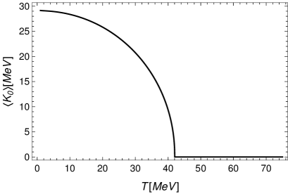
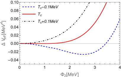
In Fig. 11 we show how the VEV associated with the field (e.g., with ) changes with the temperature. The transition temperature found in the context of the the OPT is MeV. This result completely agrees with the one found in figure 2 of Ref. Tran:2008mvg . For comparison purposes, we also show in Fig. 12 the way that the effective thermodynamic potential changes along the field direction. We have considered a variation of MeV around the critical temperature. The phase transition is found to be of second-order, which is also in agreement to the results shown in Fig. 3 of Ref. Tran:2008mvg .
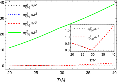
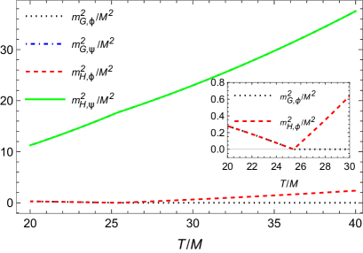
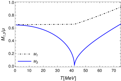
The self-consistent kaon masses discussed in Refs. Alford:2007qa ; Andersen:2008tn ; Tran:2008mvg are equivalently expressed in terms of the Eqs. (31) and (32), which we have defined previously. In the notation used in Refs. Alford:2007qa ; Andersen:2008tn ; Tran:2008mvg , they can be identified with their self-consistent masses and (note that in Ref. Andersen:2008tn , they identify with and with instead). These self-consistent masses are shown in Fig. 13.
An issue of particular importance discussed in Refs. Alford:2007qa ; Andersen:2008tn ; Tran:2008mvg , was the difficulty of the Goldstone theorem to be satisfied in the CJT formalism. Slight variations of implementation of the CJT in those references have been proposed in order for the Goldstone theorem to be satisfied at least in an approximate form. As we have already discussed in the previous sections, in the OPT formalism, as seen explicitly at the order of the OPT considered in the previous section, the Goldstone theorem is satisfied exactly. As we have already demonstrated the validity of the Goldstone theorem through the mass eigenvalues defined in the previous sections and exemplified, e.g., by Figs. 6 and 8, we refrain here from doing the same thing, but using simply a different set of parameters.
Finally, we can also implement the constrain of charge neutrality for the kaon system in the same manner as discussed in Refs. Alford:2007qa ; Andersen:2008tn ; Tran:2008mvg . This is of particular importance when applying the results for bulk matter in compact stars, where there is overall color and electrical charges neutrality. By assuming an ideal Fermi gas for the background of electrons, charge neutrality can be implemented by adding to the Lagrangian density Eq. (37) the contribution from the electrons,
| (38) |
where here denotes the Dirac field for the electron, the electron charge, the chemical potential and the electron mass. The additional contribution for the thermodynamic potential, in the high temperature approximation , is simply
| (39) |
for which the electron charge density gives,
| (40) |
The overall charge neutrality for the system imposes the constraint (recalling the we are associating the complex scalar field with the charged kaon)
| (41) |
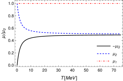
In Fig. 14, we show the chemical potentials associated with the kaons and electron as a function of the temperature. This result can be contrasted for instance with the Fig. 7 in Ref. Alford:2007qa or Fig. 1 in Ref. Tran:2008mvg .
V Conclusions
In this paper we have studied the question of achieving symmetry inversion and symmetry persistence, ISB and SNR, respectively, at high temperatures when finite charges are taken into account. The results were studied by making use of the nonperturbative OPT method, which has already been used successfully before in many other different contexts.
We have shown that the chemical potential for the fields tends to favor both ISB and SNR phenomena in the context of a two complex scalar field system. This happens such that, for instance, the critical temperature for ISB becomes smaller the larger are the chemical potentials for the fields. When studying the same system at finite density charges, we have followed the pioneering work considered in Refs. Bernstein:1990kf ; Benson:1991nj , which studied the one complex scalar field case. By working with a fixed charge density over entropy density ratio, which is motivated for example in cosmological settings, we have demonstrated that charges densities further facilitate both ISB and SNR. The finite density effects allow for both fields to experience ISB or SNR, which is not allowed in the absence of conserved charges. Our results, thus, extend to multiple coupled complex scalar field systems the study originally performed only in the one complex field case.
Finally, as an application of our results and the OPT method used in our study, we have considered the condensation of kaons, as expected, e.g., in a CFL phase of QCD at large densities. We have contrasted our results with similar ones previously considered in the literature, but which made use of the CJT nonperturbative method. Our results with the OPT, besides of comparing favorable with those obtained with the CJT method, have the additional advantage of being simpler in implementing and at the same time fully satisfying the Goldstone theorem, which has been a particular issue in the other nonperturbative methods.
Acknowledgements.
R.O.R. would like to acknowledge the McGill University Physics Department for the hospitality. The authors acknowledge financial support from Coordenação de Aperfeiçoamento de Pessoal de Nível Superior (CAPES) - Finance Code 001 and by research grants from Conselho Nacional de Desenvolvimento Científico e Tecnológico (CNPq), Grant No. 307286/2021-5 (R.O.R) and No. 309598/2020-6 (R.L.S.F.), from Fundação Carlos Chagas Filho de Amparo à Pesquisa do Estado do Rio de Janeiro (FAPERJ), Grant No. E-26/201.150/2021 (R.O.R.) and from FAPERGS Grants Nos. 19/2551-0000690-0 and 19/2551-0001948-3 (R.L.S.F.).Appendix A The ETP to first order in the OPT
Let us explicitly derive each one of the terms in Fig. 1 and which contribute to the ETP at first order in the OPT. We work in Euclidean space, with momentum square denoted by , where , and are the Matsubara’s frequencies for bosons. All momenta integrals are evaluated in dimensional regularization in the scheme. Hence, the momentum integrals in the loop contributions at finite temperature and chemical potential are represented by
| (42) |
where is the chemical potential associated with the field. The divergent vacuum momentum integral terms are regularized in the scheme, with , is the Euler-Mascheroni constant, , and is the arbitrary mass regularization scale. The sum in Eq. (42) is performed over the Matsubara’s frequencies.
Performing the sum over the Matsubara’s frequencies and the momentum integrals in dimensional regularization, we have for instance that
| (43) |
and
| (44) |
where
| (45) |
and
| (46) |
with and denoting the thermal integrals, are defined as
| (47) | |||||
and
Note that in the notation of Harber and Welson, Ref. Haber:1981tr , the thermal integrals in Eqs. (47) and (LABEL:IB), are given, respectively, by
| (49) |
and
| (50) |
where and . As shown in Ref. Haber:1981tr , the thermal functions have a high temperature expansion given by
where is the Digama function, and are hypergeometric functions, is the Riemann zeta function and is the Gamma function.
Individually, each diagram shown in Fig. 1, after performing the sum over the Matsubara’s frequencies and the momentum integrals for the vacuum terms, is then explicitly given by
| (52) | |||||
| (53) | |||||
| (54) | |||||
| (55) | |||||
| (56) | |||||
| (57) | |||||
| (58) | |||||
| (59) | |||||
| (60) | |||||
| (61) | |||||
| (62) | |||||
where in the above expressions, we have also defined
| (63) |
The divergent terms in Eqs. (56)-(59) can be eliminated by introducing the mass counterterms in the OPT Lagrangian density Eq. (9) by redefining the bare quadratic OPT masses as and , where the counterterms and are given, respectively, by
| (64) | |||||
| (65) |
These mass counterterms then give the explicit additional contributions at order ,
| (66) | |||||
| (67) |
The mass counterterms also enter as additional vertices, just like in the standard perturbation theory case, which then lead to the additional loop contributions at order ,
| (68) | |||||
| (69) | |||||
Finally, the remaining divergences are all vacuum terms, which can be canceled by adding to the OPT Lagrangian density Eq. (9) a vacuum renormalization counterterm,
| (70) | |||||
Note that at first order in the OPT there are no vertex counterterms that are required. Vertex counterterms do appear though when carrying out the OPT at second order and higher orders (see, e.g., Refs. Pinto:1999py ; Farias:2008fs ).
Putting all terms together, we find the renormalized ETP in the OPT at first order as given by Eq. (13) in the text.
Appendix B Energy spectrum and the mass eigenvalues
By shifting the fields around their background expectation values, and in the Lagrangian density Eq. (2), the quadratic part of the Lagrangian density in the fluctuation fields, , reads like
| (75) |
where is the matrix of quadratic coefficients. In the Euclidean momentum representation it gives the free inverse propagator matrix,
| (80) |
where we have defined
| (81) |
with analogous expressions for and , replacing the fields labeling in the above expression. The eigenvalues of the free inverse propagator matrix , denoted here as , , give the energy spectrum (dispersion relations) for the particles in the model. The expressions for are long and cumbersome, however, the mass eigenvalues , when taking in Eq. (80), are simple and they are given by
| (82) | |||||
| (83) | |||||
| (84) | |||||
| (85) |
Note that from the tree-level potential,
| (86) | |||||
which when it is minimized with respect to the fields, we obtain that the tree-level vacuum expectation values and , are given, respectively, by
| (87) | |||
| (88) |
When substituting and in the mass eigenvalues, we can recognize that and are, respectively, the Higgs and Goldstone modes associated with the complex scalar field , while and are, respectively, the Higgs and Goldstone modes associated with .
References
- (1) K. Huang, Statistical Mechanics (Wiley, New York, 1991).
- (2) J. I. Kapusta, Bose-Einstein Condensation, Spontaneous Symmetry Breaking, and Gauge Theories, Phys. Rev. D 24, 426-439 (1981) doi:10.1103/PhysRevD.24.426
- (3) H. E. Haber and H. A. Weldon, Thermodynamics of an Ultrarelativistic Bose Gas, Phys. Rev. Lett. 46, 1497 (1981) doi:10.1103/PhysRevLett.46.1497
- (4) H. E. Haber and H. A. Weldon, Finite Temperature Symmetry Breaking as Bose-Einstein Condensation, Phys. Rev. D 25, 502 (1982) doi:10.1103/PhysRevD.25.502
- (5) J. Bernstein and S. Dodelson, Relativistic Bose gas, Phys. Rev. Lett. 66, 683-687 (1991) doi:10.1103/PhysRevLett.66.683
- (6) K. M. Benson, J. Bernstein and S. Dodelson, Phase structure and the effective potential at fixed charge, Phys. Rev. D 44, 2480-2497 (1991) doi:10.1103/PhysRevD.44.2480
- (7) S. Weinberg, Gauge and Global Symmetries at High Temperature, Phys. Rev. D 9, 3357-3378 (1974) doi:10.1103/PhysRevD.9.3357
- (8) P. M. Stevenson, Optimized Perturbation Theory, Phys. Rev. D 23, 2916 (1981) doi:10.1103/PhysRevD.23.2916
- (9) A. Okopinska, Nonstandard expansion techniques for the effective potential in quantum field theory, Phys. Rev. D 35, 1835-1847 (1987) doi:10.1103/PhysRevD.35.1835
- (10) K. G. Klimenko, Nonlinear optimized expansion and the Gross-Neveu model, Z. Phys. C 60, 677-682 (1993) doi:10.1007/BF01558396
- (11) H. Kleinert, Strong coupling theory in four epsilon dimensions, and critical exponents, Phys. Rev. D 57, 2264-2278 (1998) doi:10.1103/PhysRevD.58.107702
- (12) S. Chiku and T. Hatsuda, Optimized perturbation theory at finite temperature, Phys. Rev. D 58, 076001 (1998) doi:10.1103/PhysRevD.58.076001 [arXiv:hep-ph/9803226 [hep-ph]].
- (13) M. B. Pinto and R. O. Ramos, High temperature resummation in the linear delta expansion, Phys. Rev. D 60, 105005 (1999) doi:10.1103/PhysRevD.60.105005 [arXiv:hep-ph/9903353 [hep-ph]].
- (14) M. B. Pinto and R. O. Ramos, A Nonperturbative study of inverse symmetry breaking at high temperatures, Phys. Rev. D 61, 125016 (2000) doi:10.1103/PhysRevD.61.125016 [arXiv:hep-ph/9912273 [hep-ph]].
- (15) R. L. S. Farias, G. Krein and R. O. Ramos, Applicability of the Linear delta Expansion for the Field Theory at Finite Temperature in the Symmetric and Broken Phases, Phys. Rev. D 78, 065046 (2008) doi:10.1103/PhysRevD.78.065046 [arXiv:0809.1449 [hep-ph]].
- (16) V. I. Yukalov, Interplay between Approximation Theory and Renormalization Group, Phys. Part. Nucl. 50, no.2, 141-209 (2019) doi:10.1134/S1063779619020047 [arXiv:2105.12176 [hep-th]].
- (17) D. Curtin, P. Meade and H. Ramani, Thermal Resummation and Phase Transitions, Eur. Phys. J. C 78, no.9, 787 (2018) doi:10.1140/epjc/s10052-018-6268-0 [arXiv:1612.00466 [hep-ph]].
- (18) D. Croon, O. Gould, P. Schicho, T. V. I. Tenkanen and G. White, Theoretical uncertainties for cosmological first-order phase transitions, JHEP 04, 055 (2021) doi:10.1007/JHEP04(2021)055 [arXiv:2009.10080 [hep-ph]].
- (19) E. Senaha, Symmetry Restoration and Breaking at Finite Temperature: An Introductory Review, Symmetry 12, no.5, 733 (2020) doi:10.3390/sym12050733
- (20) P. M. Schicho, T. V. I. Tenkanen and J. Österman, Robust approach to thermal resummation: Standard Model meets a singlet, JHEP 06, 130 (2021) doi:10.1007/JHEP06(2021)130 [arXiv:2102.11145 [hep-ph]].
- (21) O. Gould and T. V. I. Tenkanen, On the perturbative expansion at high temperature and implications for cosmological phase transitions, JHEP 06, 069 (2021) doi:10.1007/JHEP06(2021)069 [arXiv:2104.04399 [hep-ph]].
- (22) M. G. Alford, K. Rajagopal and F. Wilczek, Color flavor locking and chiral symmetry breaking in high density QCD, Nucl. Phys. B 537, 443-458 (1999) doi:10.1016/S0550-3213(98)00668-3 [arXiv:hep-ph/9804403 [hep-ph]].
- (23) M. G. Alford, A. Schmitt, K. Rajagopal and T. Schäfer, Color superconductivity in dense quark matter, Rev. Mod. Phys. 80, 1455-1515 (2008) doi:10.1103/RevModPhys.80.1455 [arXiv:0709.4635 [hep-ph]].
- (24) M. G. Alford, M. Braby and A. Schmitt, Critical temperature for kaon condensation in color-flavor locked quark matter, J. Phys. G 35, 025002 (2008) doi:10.1088/0954-3899/35/2/025002 [arXiv:0707.2389 [nucl-th]].
- (25) J. O. Andersen and L. E. Leganger, Kaon condensation in the color-flavor-locked phase of quark matter, the Goldstone theorem, and the 2PI Hartree approximation, Nucl. Phys. A 828, 360-389 (2009) doi:10.1016/j.nuclphysa.2009.07.003 [arXiv:0810.5510 [hep-ph]].
- (26) H. P. Tran, V. Nguyen, T. A. Nguyen and V. H. Le, Kaon condensation in the linear sigma model at finite density and temperature, Phys. Rev. D 78, 105016 (2008) doi:10.1103/PhysRevD.78.105016
- (27) J. M. Cornwall, R. Jackiw and E. Tomboulis, Effective Action for Composite Operators, Phys. Rev. D 10, 2428-2445 (1974) doi:10.1103/PhysRevD.10.2428
- (28) G. Amelino-Camelia and S. Y. Pi, Selfconsistent improvement of the finite temperature effective potential, Phys. Rev. D 47, 2356-2362 (1993) doi:10.1103/PhysRevD.47.2356 [arXiv:hep-ph/9211211 [hep-ph]].
- (29) J. I. Kapusta and C. Gale, Finite-temperature field theory: Principles and applications, Cambridge University Press, 2011, ISBN 978-0-521-17322-3, 978-0-521-82082-0, 978-0-511-22280-1 doi:10.1017/CBO9780511535130
- (30) D. S. Rosa, R. L. S. Farias and R. O. Ramos, Reliability of the optimized perturbation theory in the 0-dimensional scalar field model, Physica A 464, 11-26 (2016) doi:10.1016/j.physa.2016.07.067 [arXiv:1604.00537 [hep-ph]].
- (31) R. L. S. Farias, R. O. Ramos and D. S. Rosa, Symmetry breaking patterns for two coupled complex scalar fields at finite temperature and in an external magnetic field, Phys. Rev. D 104, no.9, 096011 (2021) doi:10.1103/PhysRevD.104.096011 [arXiv:2109.03671 [hep-ph]].
- (32) D. C. Duarte, R. L. S. Farias and R. O. Ramos, Optimized perturbation theory for charged scalar fields at finite temperature and in an external magnetic field, Phys. Rev. D 84, 083525 (2011) doi:10.1103/PhysRevD.84.083525 [arXiv:1108.4428 [hep-ph]].
- (33) C. H. Lee, Kaon condensation in dense stellar matter, Phys. Rept. 275, 255-341 (1996) doi:10.1016/0370-1573(96)00005-1
- (34) D. T. Son and M. A. Stephanov, Inverse meson mass ordering in color flavor locking phase of high density QCD, Phys. Rev. D 61, 074012 (2000) doi:10.1103/PhysRevD.61.074012 [arXiv:hep-ph/9910491 [hep-ph]].
- (35) D. B. Kaplan and S. Reddy, Novel phases and transitions in color flavor locked matter, Phys. Rev. D 65, 054042 (2002) doi:10.1103/PhysRevD.65.054042 [arXiv:hep-ph/0107265 [hep-ph]].
- (36) T. Schäfer, Instanton effects in QCD at high baryon density, Phys. Rev. D 65, 094033 (2002) doi:10.1103/PhysRevD.65.094033 [arXiv:hep-ph/0201189 [hep-ph]].
- (37) H. E. Haber and H. A. Weldon, On the Relativistic Bose-einstein Integrals, J. Math. Phys. 23, 1852 (1982) doi:10.1063/1.525239