Phononic-crystal cavity magnomechanics
Abstract
Establishing a way to control magnetic dynamics and elementary excitations (magnons) is crucial to fundamental physics and the search for novel phenomena and functions in magnetic solid-state systems. Electromagnetic waves have been developed as means of driving and sensing in magnonic and spintronics devices used in magnetic spectroscopy, non-volatile memory, and information processors Jungwirth et al. (2012); Chumak et al. (2015); Tabuchi et al. (2015); Li et al. (2020); Awschalom et al. (2021). However, their millimeter-scale wavelengths and undesired cross-talk have limited operation efficiency and made individual control of densely integrated magnetic systems difficult. Here, we utilize acoustic waves (phonons) to control magnetic dynamics in a miniaturized phononic crystal micro-cavity and waveguide architecture. We demonstrate acoustic pumping of localized ferromagnetic magnons, where their back-action allows dynamic and mode-dependent modulation of phononic cavity resonances. The phononic crystal platform enables spatial driving, control and read-out of tiny magnetic states and provides a means of tuning acoustic vibrations with magnons. This alternative technology enhances the usefulness of magnons and phonons for advanced sensing, communications and computation architectures that perform transduction, processing, and storage of classical and quantum information Chumak et al. (2015); Awschalom et al. (2021).
Acoustic phonons are possibly means for controlling magnons on-chip because of their micro-/nanometer wavelengths (similar to those of magnons), low-loss property, and negligible cross-talk Li et al. (2021); Zhang et al. (2016); Kikkawa et al. (2016); Berk et al. (2019); An et al. (2020); Potts et al. (2021). The pioneering studies on magnomechanical technology used surface acoustic wave (SAW) devices Weiler et al. (2011); Dreher et al. (2012); Kobayashi et al. (2017); Sasaki et al. (2017); Hernndez-Mnguez
et al. (2020); Xu et al. (2020); Kawada et al. (2021); Hatanaka et al. (2022). They succeeded in generating various magnetoelastic phenomena like acoustic spin pumping Kobayashi et al. (2017); Matsuo et al. (2013) and nonreciprocal transport Sasaki et al. (2017); Xu et al. (2020). However, their large cavity structures are unsuitable for system integration and have difficulty taking full advantage of phonons Hatanaka et al. (2022).
A phononic crystal (PnC) is a promising platform that enables acoustic phonons to be guided and trapped in a tiny wavelength-scale acoustic cavity and waveguide Maldovan (2013); Benchabane et al. (2006); Mohammadi et al. (2009); Otsuka et al. (2013); Pourabolghasem
et al. (2018); Baboly et al. (2018); Hatanaka and Yamaguchi (2020). Individual cavities are efficiently and finely driven and thereby can be used to control magnetic elements embedded in a PnC circuit. Moreover, the cavity sustains various spatial distributions of vibrational strains among multiple acoustic resonances, so it can be used to adjust the magnetoelastic effect Hatanaka and Yamaguchi (2021). We consider that PnCs will enable us to make full use of phonons in magnomechanical technology.
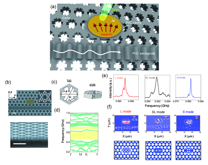
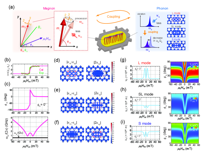
Here, we demonstrate a PnC-based magnomechanical system sustained by cavity-waveguide coupled systems, as shown in Fig. 1(a). The nanomechanical vibrations confined in the cavity, excited through the waveguide, generate spin waves (magnons) in a nickel (Ni) film placed on its surface via magnetostriction. The acoustic spin pumping reversibly induces a frequency shift and damping modulation of the cavity resonances. Moreover, the magnon-phonon interaction can be tailored by selectively driving an appropriate cavity mode with specific strain distributions. PnC cavity magnomechanics is useful for on-chip control of magnons and phonons as well as their hybridized states (magnon polaron), and shows promise for extending the capabilities of classical and quantum information technologies.
The PnC is fabricated in free-standing GaAs, as shown in Fig.1(b) (the details of the fabrication and structure are presented in the Methods.). It consists of a snowflake triangular lattice with full bandgaps between 0.5 and 0.8 GHz (Fig. 1(c) and 1(d)) Hatanaka and Yamaguchi (2020); Safavi-Naeini et al. (2014). Acoustic waves at frequencies within the bandgap propagate in a line-defect waveguide and drive a line-defect cavity. Measuring the cavity’s spectral response reveals three acoustic resonances (Fig. 1(e)). Their modal shapes exhibit complete confinement of the vibrations in the defect (top panels of Fig. 1(f)). Numerical calculations with the finite-element method (FEM) reproduce these modal shapes and verify the origin of the observed peaks. In this way, the PnC cavity can strongly confine vibrations that are remotely driven through the waveguide.
The Ni film on the cavity surface has a magnetization whose precession is acoustically excited via magnetostriction. The magnetostrictive force that induces the precession is divided into two components and on the - and -axis, whose definitions are given in Fig. 2(a). The equilibrium magnetization axis () can be decomposed into in-plane and components and is at an angle () from the waveguide direction . The out-of-plane magnetostrictive force () is negligibly small because out-of-plane shear strains such as and vanish in the Ni at that location, whereas in-plane force () can be expressed as Dreher et al. (2012)
| (1) |
where is the magnetostrictive coefficient and is the vibrational strain component. Thus, the magnetostriction is governed by two major factors, vibrational strain (, and ) and the magnetization direction (), whose contributions to the system are theoretically investigated below.
The magnetization angle () can be predicted from the magnetic free-energy density normalized by the saturation magnetization (), given by Dreher et al. (2012)
| (2) |
where and are the external magnetic field and unit vector of magnetization, respectively. The thin-film structure of the Ni results in a perpendicular magnetic anisotropy (). The angle is determined by estimating the minimum of . In this calculation, the in-plane anisotropic field () and its unit vector () are introduced so as to reproduce the experimental magnetization curve (Fig. 2(b)). For instance, the response of as a function of at = 0∘ is shown in the top panel of Fig. 2(c). The magnetization is parallel to , i.e. , when the field strength stays in the high field region 20 mT. However, it undergoes a rotation to in the low field region 20 mT before reversing. In this way, the magnetization experiences a rotation and reversal while sweeping . This change in magnetization determines the magnon resonance frequency (). The field response is shown in the bottom panel of Fig. 2(c). The frequency monotonically decreases with decreasing and approaches the acoustic resonant frequency () at = 7 mT, where the magnon-phonon frequency mismatch is minimized.
Another aspect determining the magnetostriction is the spatial distribution and direction of vibration strains. The observed acoustic resonances can be decomposed into three strain components (Fig. 2(d)-2(f) shows the spatial profiles of the longitudinal () and shear strain components () of the resonances). Shear (longitudinal) strain is dominant in the resonances at 0.581 GHz (0.593 GHz), whereas both strains are comparable at 0.552 GHz. The desired strain distributions can thus be generated by selectively actuating an appropriate resonance. Hereafter, the shear- and longitudinal-strain modes will be labeled S and L, while the mode with comparable strains will be labeled SL.
The magnetization dynamics and spatial strain profiles allow us to estimate the magnetostrictive coupling mode volume (), which characterizes the interaction efficiency. determined by and the magnon-phonon spatial mode overlap (expression and derivation in the Methods). Figures 2(g)-2(i) show the simulated field dependence of of the L, SL, and S modes at = 0∘ and for various between and . For the L mode at , mostly vanishes in the high field region because and is negligibly small. In contrast, it increases dramatically as decreases below 20 mT. This enhancement at mT is caused by the magnetization rotation from = 0∘ to 45∘; thereby, the term becomes non-zero. temporarily returns to almost zero as reaches 90∘ just before the magnetization reverses and then approaches the original value after the increase at and mT. In contrast, the S mode exhibits the opposite field dependency, in which a finite in the high field region is reduced in the low field region because the dominant magnetostrictive term is , not . Since the SL mode has almost equal contributions from both strain components, the variation with respect to is moderate compared with the other two modes (Methods). As increases, the susceptibility to is cyclically modulated (right panels of Fig. 2(g)-2(i)). The change in direction of while sweeping is opposite between S and L modes, resulting from different dominant strain components. These results indicate that the cavity mode structures as well as the external field can be used to tune the magnetostrictive interaction.
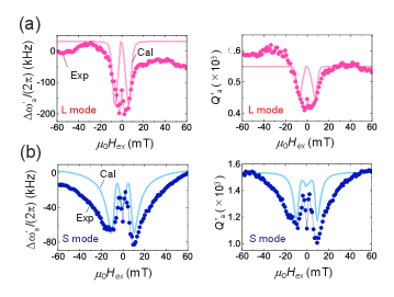
To experimentally show the magnetostrictive interaction, the field response of the cavity resonance was measured at . The observed resonant frequency shift () and quality factor () are plotted as a function of in Fig. 3(a) and 3(b), where L and S modes are chosen for their opposite and distinct field susceptibilities. The response on the L mode exhibits dual dips at = 5 mT with a reduction in and in the low field region. This behavior can be understood from the theoretical formula,
| (3) |
where , , and are mass density, acoustic mode volume, driving force density and angular frequency, and is magnetic susceptibility (Methods). The theoretical predictions are in agreement with the experimental results, indicating that the acoustic modulation is due to the magnon-phonon interaction, as described by our model. This interaction enables acoustic excitation of spin-wave oscillations in Ni, which exerts back-action force on the cavity resonance and tunes and .
Remarkably, ferromagnetic magnons were able to be driven by phonons in the tiny PnC cavity. The effective mode volume of the L mode is estimated to be m3 = 0.54 with an acoustic wavelength of 3.5 m, which is times smaller than that of a SAW-based magnomechanical cavity system Hatanaka et al. (2022). The tiny-energy vibrations are confined by the high resonance, so they hardly affect surrounding systems, unlike conventional electromagnetic-wave-based magnetic devices. We believe that the PnC cavity-waveguide system would be a building block for a magnomechanical system and could be used as a local magnon driver and phonon modulator.
Strong back-action effects were also observed in the S mode, where shear strain dominate magnetostriction. A comparison with the effect in the L mode reveals the impact of the mode strain profiles on the interaction. Figure 3(b) shows that the dual dips in this mode at = 10 mT are wider than those in the L mode because of the finite in the high field region. In addition, a distinct center dip occurs around mT, an effect of the magnetization rotation. The field response is distinctly different from that in the L mode and can be simulated with our model. Thus, our cavity geometry is also used to selectively drive the magnetization dynamics utilizing the difference in strain distributions.
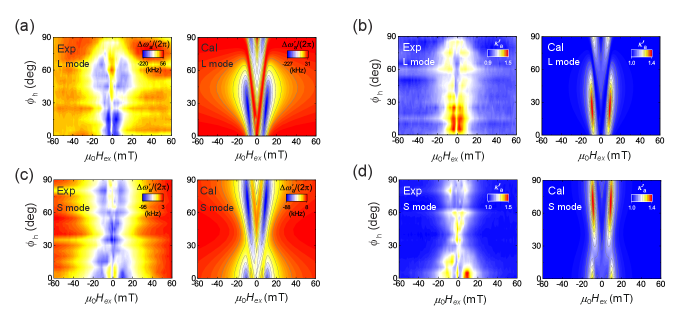
To examine how the strain distribution affects the magnetoelastic modulation, the field responses of the acoustic resonant frequency () and damping rate () on the L and S modes were investigated at ranging from to (Fig. 4(a)-4(d)). The magnetoelastic modulation regions in and broaden as increases from 0∘ to 60∘ in the L mode and shrink toward = 90∘. In contrast, the S mode shows the opposite dependency, in which the modulation regions become narrow around = 45∘. The theoretical calculations reproduce the experimental variations in both modes; here, the cyclic modulation while changing is governed by , so the L and S modes show the opposite behaviors. Note that the experiment and theoretical model showed a moderate response to the magnetoelastic effect in the SL mode (Methods), supporting the validity of our model. We also found similar mode-sensitive magnetoelastic modulation in a PnC cavity with a different defect geometry (Methods). These results verify that the mode-tunable magnetostriction allows us to control magnomechanical states acoustically.
In conclusion, the ease of designing the PnC cavity and the small spatial leakage of its vibrations are useful for constructing integrated magnomechanical systems, in which microwave signal operations such as sensing, memory and processing are performed using magnons and phonons. Moreover, it is possible to build a tiny magnomechanical system of magnon wavelength size to efficiently control and read-out the magnetic state of a micro-/nano-ferromagnetic system such as a magnetic tunnel junction Yuasa et al. (2004). We believe that PnC cavity magnomechanics will expand the use of magnons and phonons and related technologies.
Acknowledgments
This work was partially supported by JSPS KAKENHI(S) Grant Number JP21H05020.
Author contributions
D.H. fabricated the device and performed the measurements and the data analysis. M.A. made theoretical model, and D.H. and M.A conducted the simulations with support from H. Y. and H.O.. D.H. and M.A. wrote the manuscript. All authors discussed the results during preparation of the paper.
References
- Jungwirth et al. (2012) T. Jungwirth, J. Wunderlich, and K. Olejník. Spin hall effect devices. Nature materials 11, 382 (2012).
- Chumak et al. (2015) A. V. Chumak, V. I. Vasyuchka, A. A. Serga, and B. Hillebrands. Magnon spintronics. Nature Physics 11, 453 (2015).
- Tabuchi et al. (2015) Y. Tabuchi, S. Ishino, A. Noguchi, T. Ishikawa, R. Yamazaki, K. Usami, and Y. Nakamura. Coherent coupling between a ferromagnetic magnon and a superconducting qubit. Science 349, 405 (2015).
- Li et al. (2020) Y. Li, W. Zhang, V. Tyberkevych, W.-K. Kwok, A. Hoffmann, and V. Novosad. Hybrid magnonics: Physics, circuits, and applications for coherent information processing. Journal of Applied Physics 128, 130902 (2020).
- Awschalom et al. (2021) D. D. Awschalom, C. Du, R. He, J. Heremans, A. Hoffmann, J. Hou, H. Kurebayashi, Y. Li, L. Liu, V. Novosad, et al. Quantum engineering with hybrid magnonics systems and materials. IEEE Transactions on Quantum Engineering (2021).
- Li et al. (2021) Y. Li, C. Zhao, W. Zhang, A. Hoffmann, and V. Novosad. Advances in coherent coupling between magnons and acoustic phonons. APL Mater. 9, 060902 (2021).
- Zhang et al. (2016) X. Zhang, C.-L. Zou, L. Jiang, and H. X. Tang. Cavity magnomechanics. Sci. Adv. 2, e1501286 (2016).
- Kikkawa et al. (2016) T. Kikkawa, K. Shen, B. Flebus, R. A. Duine, K.-i. Uchida, Z. Qiu, G. E. Bauer, and E. Saitoh. Magnon polarons in the spin seebeck effect. Phys. Rev. Lett. 117, 207203 (2016).
- Berk et al. (2019) C. Berk, M. Jaris, W. Yang, S. Dhuey, S. Cabrini, and H. Schmidt. Strongly coupled magnon–phonon dynamics in a single nanomagnet. Nature communications 10, 1 (2019).
- An et al. (2020) K. An, A. N. Litvinenko, R. Kohno, A. A. Fuad, V. V. Naletov, L. Vila, U. Ebels, G. de Loubens, H. Hurdequint, N. Beaulieu, et al. Coherent long-range transfer of angular momentum between magnon kittel modes by phonons. Phys. Rev. B 101, 060407(R) (2020).
- Potts et al. (2021) C. A. Potts, E. Varga, V. A. Bittencourt, S. V. Kusminskiy, and J. P. Davis. Dynamical backaction magnomechanics. Physical Review X 11, 031053 (2021).
- Weiler et al. (2011) M. Weiler, L. Dreher, C. Heeg, H. Huebl, R. Gross, M. S. Brandt, and S. T. B. Goennenwein. Elastically driven ferromagnetic resonance in nickel thin films. Phys. Rev. Lett. 106, 117601 (2011).
- Dreher et al. (2012) L. Dreher, M. Weiler, M. Pernpeintner, H. Huebl, R. Gross, M. S. Brandt, and S. T. B. Goennenwein. Surface acoustic wave driven ferromagnetic resonance in nickel thin films: Theory and experiment. Phys. Rev. B 86, 134415 (2012).
- Kobayashi et al. (2017) D. Kobayashi, T. Yoshikawa, M. Matsuo, R. Iguchi, S. Maekawa, E. Saitoh, and Y. Nozaki. Spin current generation using a surface acoustic wave generated via spin-rotation coupling. Phys. Rev. Lett. 119, 077202 (2017).
- Sasaki et al. (2017) R. Sasaki, Y. Nii, Y. Iguchi, and Y. Onose. Nonreciprocal propagation of surface acoustic wave in ni/linbo 3. Physical Review B 95, 020407 (2017).
- Hernndez-Mnguez et al. (2020) A. Hernndez-Mnguez, F. Maci, J. M. Hernndez, J. Herfort, and P. V. Santos. Large nonreciprocal propagation of surface acoustic waves in epitaxial ferromagnetic/semiconductor hybrid structures. Phys. Rev. Appl. 13, 044018 (2020).
- Xu et al. (2020) M. Xu, K. Yamamoto, J. Puebla, K. Baumgaertl, B. Rana, K. Miura, H. Takahashi, D. Grundler, S. Maekawa, and Y. Otani. Nonreciprocal surface acoustic wave propagation via magneto-rotation coupling. Science Adv. 6, eabb1724 (2020).
- Kawada et al. (2021) T. Kawada, M. Kawaguchi, T. Funato, H. Kohno, and M. Hayashi. Acoustic spin hall effect in strong spin-orbit metals. Sci. Adv. 7, eabd9697 (2021).
- Hatanaka et al. (2022) D. Hatanaka, M. Asano, H. Okamoto, T. Kunihashi, H. Sanada, and H. Yamaguchi. On-chip coherent transduction between magnons and acoustic phonons in cavity magnomechanics. Physical Review Applied 17, 034024 (2022).
- Matsuo et al. (2013) M. Matsuo, J. Ieda, K. Harii, E. Saitoh, and S. Maekawa. Mechanical generation of spin current by spin-rotation coupling. Physical Review B 87, 180402 (2013).
- Maldovan (2013) M. Maldovan. Sound and heat revolutions in phononics. Nature 503, 209 (2013).
- Benchabane et al. (2006) S. Benchabane, A. Khelif, J.-Y. Rauch, L. Robert, and V. Laude. Evidence for complete surface wave band gap in a piezoelectric phononic crystal. Phys. Rev. E 73, 065601(R) (2006).
- Mohammadi et al. (2009) S. Mohammadi, A. A. Eftekhar, W. D. Hunt, and A. Adibi. High- micromechanical resonators in a two-dimensional phononic crystal slab. Appl. Phys. Lett. 94, 051906 (2009).
- Otsuka et al. (2013) P. H. Otsuka, K. Nanri, O. Matsuda, M. Tomoda, D. M. Profunser, I. A. Veres, S. Danworaphong, A. Khelif, S. Benchabane, V. Laude, et al. Broadband evolution of phononic-crystal-waveguide eigenstates in real- and k-spaces. Sci. Rep. 3, 3351 (2013).
- Pourabolghasem et al. (2018) R. Pourabolghasem, R. Dehghannasiri, A. A. Eftekhar, and A. Adibi. Waveguiding effect in the gigahertz frequency range in pillar-based phononic-crystal slabs. Phys. Rev. Appl. 9, 014013 (2018).
- Baboly et al. (2018) M. G. Baboly, C. M. Reinke, B. A. Griffin, I. El-Kady, and Z. C. Leseman. Acoustic waveguiding in a silicon carbide phononic crystals at microwave frequencies. Appl. Phys. Lett. 112, 103504 (2018).
- Hatanaka and Yamaguchi (2020) D. Hatanaka and H. Yamaguchi. Real-space characterization of cavity-coupled waveguide systems in hypersonic phononic crystals. Phys. Rev. Appl. 13, 024005 (2020).
- Hatanaka and Yamaguchi (2021) D. Hatanaka and H. Yamaguchi. Mode-sensitive magnetoelastic coupling in phononic-crystal magnomechanics. APL Materials 9, 071110 (2021).
- Safavi-Naeini et al. (2014) A. H. Safavi-Naeini, J. T. Hill, S. Meenehan, J. Chan, S. Grblacher, and O. Painter. Two-dimensional phononic-photonic band gap optomechanical crystal cavity. Phys. Rev. Lett. 112, 153603 (2014).
- Yuasa et al. (2004) S. Yuasa, T. Nagahama, A. Fukushima, Y. Suzuki, and K. Ando. Giant room-temperature magnetoresistance in single-crystal Fe/MgO/Fe magnetic tunnel junctions. Nature materials 3, 868 (2004).
Methods
Appendix A Fabrication and measurement
The magnomechanical PnC was fabricated from GaAs (1.0 m)/ Al0.7Ga0.3As (3.0 m) heterostructure on a GaAs single-crystalline substrate. A periodic arrangement of snowflake-shaped air holes was formed by electron-beam lithography and dry etching. The GaAs layer, including the PnC lattice, was suspended by immersion in diluted hydrofluoric acid (5). The PnC geometry gives rise to a complete bandgap between 0.45-0.60 GHz and 0.65-0.71 GHz. The acoustic waveguide was constructed by removing one line from the lattice, thereby enabling single-mode propagation at frequencies within the bandgap Hatanaka and Yamaguchi (2020). The resonator (cavity) formed by removing two holes was located at one side of the waveguide and sustains multiple resonant vibrations. A ferromagnetic thin film of nickel (Ni) with a thickness of 50 nm was deposited on the surface of the cavity and holds spin-wave (magnon) resonances. 5-nm-thick gold (Au) film was deposited on the Ni layer for preventing oxidization. The free-standing PnC slab is sandwiched by inter-digit transducers (IDT) made from Cr (5 nm) / Au (35 nm). The IDT consists of 100 transducers arrayed with a period of 4.9 m 5.2 m.
Acoustic waves were piezoelectrically excited by applying alternating voltages to one IDT and optically measured with an optical interferometer (Neoark, MLD-101). The data on spectral response of the PnC cavity were obtained with a time-gating technique with a network analyzer (Keysight E5080A) to remove undesired electrical cross-talk signals. The acoustic resonance frequencies () and quality factor () in Fig. 3(a) and 3(b) were obtained by making Lorentzian or exponential fittings to the spectral and temporal response results. The acoustic damping rates (, ) in Fig. 4(b) and 4(d) were estimated from both and . The displacement amplitudes of the resonant mode profiles depicted in Fig. 1(f) were collected through frequency down-conversion followed by filtering with a lock-in amplifier (Stanford Research Systems, SR844). All experiments in this work were performed in a moderate vacuum ( Pa) and at room temperature.
Appendix B Theory of magnetoelastic dyanmics in a phononic crystal cavity
The equation of motion of the acoustic mode is given by
| (4) |
where
| (5) |
is the magnetoelastic energy density. The magnetoelastic force density in the second term on the right-hand side is given by
| (6) | ||||
In our setup, the magnetization is aligned in-plane of the Ni film and the field angle away from the -axis is defined as . Therefore, the conversion between -coordinate system and -coordinate system is
| (7) |
| (8) | ||||
| (9) | ||||
| (10) |
with approximations . Accordingly, under shear strains , the magnetoelastic force density in equation (B3) becomes
| (11) |
and
| (12) |
where and are the and components of the magnetoelastic force. As a result, we can define a new magnetoelastic vector,
| (13) |
where is the normalized amplitude of magnons at position . This magnetoelastic vector contributes to the coupling constant with the spatial integration of magnons. By redefining the acoustic mode as , we find that
| (14) |
where
| (15) |
is the effective mass with and
| (16) |
is the magnetostrictive coupling mode volume. Note that and are non-dimensional variables.
B.1 Equation of motion for magnon modes
The previous work by Dreher Dreher et al. (2012) derived the following equations of magnonic motion:
| (17) |
| (18) |
To determine , we have to diagonalize equations (B14) and (B15),
| (19) | ||||
| (20) |
where and . Here , , and . Finally, we obtain
| (21) |
where
| (22) |
and
| (23) |
and are defined as
| (24) | ||||
| (25) |
As a result, the equations of magnon motion becomes
| (26) |
By decomposing the temporal and spatial parts as , it can be expressed as
| (27) |
and
| (28) |
where is a wavevector defined as . Accordingly, the diagonalized equations can be simplified to
| (29) |
Importantly, we have the relationship
| (30) |
and thus, we use
| (31) |
B.2 Coupled mode equation
The above equations of motions of acoustic phonons and magnons lead to the following equation of motion of coupled modes,
| (32) | ||||
| (33) |
where the coupling mode volume has been redefined as and
| (34) |
By solving equations (B29) and (B30) with an additional driving force, , we obtain the acoustic displacement amplitude () modulated by back-action from magnons, where
| (35) |
and the magnetic susceptibility is
| (36) |
For the numerical calculation, we had to derive the value of at which the spatial function appears as the same order . This means that constant factors cancel out in their ratio. Magnetoelastic coupling coefficients () of 5 T, 6T and 10 T were used for the simulations of the SL, S and L modes, respectively. The angle of the in-plane anisotropic field was set at = 85∘, to reproduce the field response of the equilibrium magnetization as shown in Fig. 2(b). The table lists the other parameters of the calculations.
By transforming into the rotating frame of the acoustic modes, i.e., , the equation of motion of acoustic phonons becomes
| (37) |
The coupled mode equation in the frequency domain is given by
Hence, the acoustic mode spectra is
| (38) |
Apparently, the symmetrized coupling strength is
| (39) |
| mass density | 8900 kg/m3 | |
| out-of-plane shape anisotropy | 0.2 T | |
| in-plane magnetic anisotropy | 4 mT | |
| Gilbert damping factor | 0.1 | |
| saturation magnetization | 370 kA/m | |
| gyromagnetic ratio | 2.185 |
Appendix C Magnetoelastic modulation of SL mode in a PnC cavity
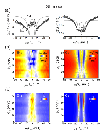
The left and right panels of Fig. 5(a) plot the resonant frequency shift () and quality factor () as functions of the bias field () for the SL mode in the . Their field responses reveal a dual dip structure due to the increased magnon-phonon interaction; the theoretical calculations (solid line) show the same dip. Compared with the other modes, the modulation magnitudes, i.e. dip depths, are small, because of the comparable contributions of the longitudinal () and shear strain components (), and thus, the field dependency of the coupling () is small. Figure 5(b) and 5(c) show the experimental (left) and simulated (right) field responses of and while sweeping from to . The field regions of the magnetoelastic modulation exhibit moderate variation with compared with the S and L modes. Clearly, the magnetoelastic dynamics are a consequence of the spatial strain distribution of this mode.
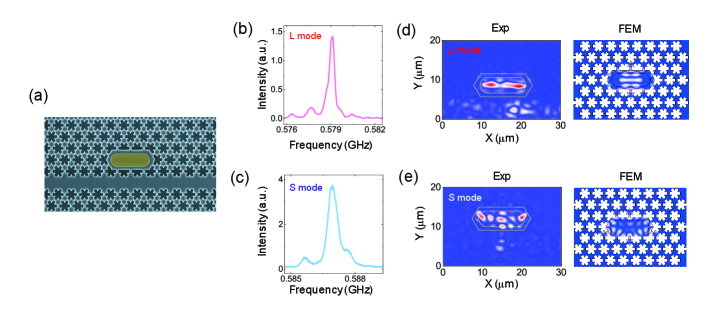
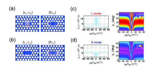
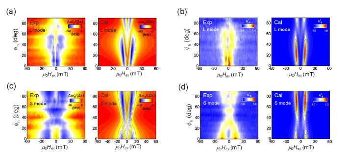
Appendix D Magnetoelastic modulation on an PnC cavity with a three-holes defect
A PnC cavity formed by removing three holes, shown in Fig. 6(a), holds two acoustic resonances at 0.579 GHz and 0.587 GHz with distinct modal shapes (Fig. 6(b) and 6(c)). These modes, labeled L and S, indicate that acoustic vibrations are confined in the defect (Fig. 6(d) and 6(e)). The numerically calculated spatial distributions of strains and are shown in the left and right panels of Fig. 7(a) and 7(b). Magnetoelastic coupling mode volume as function of the bias field strength at = 0∘ is plotted in the left panels of Fig. 7(c) and 7(d) for the L and S modes. These field responses indicate that the two modes show opposite coupling dynamics. Similarly, the field angle evolution of the response indicates the magnetoelastic modulation effect is sensitive to the field and magnetization orientation and the acoustic mode structure (right panels of Fig. 7(c) and 7(d)). Figure 8(a) and 8(c) indicate the frequency shifts of the L and S modes (left) and simulated responses (right). Figure 8(b) and 8(d) plot the normalized acoustic damping rates (left) and the simulated responses (right). The magnetoelastic coupling coefficient used in the calculations was T for both modes.