Photon echo from lensing of fractional excitations in Tomonaga-Luttinger spin liquid
Abstract
We study theoretically the nonlinear optical response of Tomonaga-Luttinger spin liquid in the context of terahertz (THz) two-dimensional coherent spectroscopy (2DCS). Using the gapless phase of the XXZ-type spin chain as an example, we show that its third-order nonlinear magnetic susceptibilities and exhibit photon echo, where refers to the left/right-hand circular polarization with respect to the axis. The photon echo arises from a “lensing” phenomenon in which the wave packets of fractional excitations move apart and then come back toward each other, amounting to a refocusing of the excitations’ world lines. Renormalization group irrelevant corrections to the fixed point Hamiltonian result in dispersion and/or damping of the wave packets, which can be sensitively detected by lensing and consequently the photon echo. Our results thus unveil the strength of THz-2DCS in probing the dynamical properties of the collective excitations in a prototypical gapless many-body system.
I Introduction
Progress in condensed matter physics is intimately connected to the development of new spectroscopic techniques. Among the many emerging spectroscopies, two-dimensional coherent spectroscopy (2DCS) stands out as a promising tool for investigating strongly correlated systems. The 2DCS use multiple coherent electromagnetic waves to probe the nonlinear optical properties of a sample, thereby producing a two-dimensional spectrum that visualizes the sample’s nonlinear response as a function of the frequencies of probing electromagnetic waves [1, 2].
Comparing to the more familiar one-dimensional spectroscopy that probes linear optical properties, the 2DCS reveals not only the optical excitations in a sample but also their relationship. In the infrared and higher frequency range, its ability to diagnose the interplay between optical excitations has been widely leveraged by chemists to unravel the structure of complex molecules and map out the kinetic pathways of chemical reactions [1, 2, 3]. The advent of terahertz (THz) 2DCS now puts this technique in the right energy window to study many-body phenomena. The THz 2DCS has offered new experimental insights into quantum wells [4], antiferromagnets [5], and electronic glasses [6]. On the theory front, it has recently been suggested that the THz 2DCS can resolve the spectral continua formed by optical excitations in several clean and disordered many-body system and characterize their dynamical properties, which would be challenging to accomplish with linear spectroscopy, if at all [7, 8, 9, 10, 11].
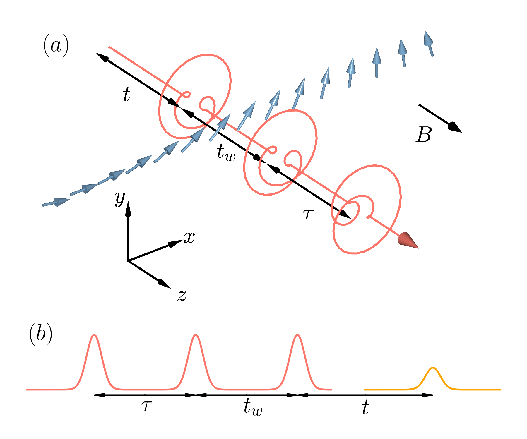
A main strength of the 2DCS lies in the photon echo [12] signal from the third-order nonlinear optical response . The photon echo is an optical analogue of the spin echo in nuclear magnetic resonance (NMR) [13]. Schematically, one may observe the photon echo by exciting the system with three successive short optical pulses and detecting the resulted response (Fig. 1(a)). Let be the time delay between the second and first pulses, (the waiting time) be the delay between the third and second, and be the delay between the time of detection and the last pulse. The photon echo signal appears as a surge of the nonlinear response at in close analogy with the nuclear magnetic resonance (NMR) spin echo (Fig. 1(b)).
Similar to its NMR cousin, the photon echo signal can diagnose dissipation in a few-body system by effecting a time-reversal operation — the system’s evolution during the time delay reverses the evolution occurred during the time delay [1, 2]. Had the dynamics been unitary, the quantum mechanical phase accumulated in would be completely removed when , resulting in a perfect rephasing. This perfect rephasing process would produce a photon echo signal at regardless the value of . Deviation from the perfect rephasing is thus a direct measure of dissipation in the few-body system. Specifically, the decay of echo signal with increasing is a manifestation of the decoherence time ( time), whereas the decay of the signal as a function of probes the population time ( time).
This unique ability of diagnosing dissipation makes one naturally wonder if the photon echo could also find its success in strongly correlated many-body systems. Although the latest theoretical inquiries have suggested interesting applications of photon echo in gapped systems [7, 8, 10] and disordered systems [9], less attention is paid to clean, gapless many-body systems. Adapting this technique to a gapless many-body setting poses new theoretical challenges. The standard framework for analyzing the photon echo uses the language of energy levels [1, 2], which is best suited for few-body systems with discrete energy spectra. While it is possible to analyze the zero temperature optical response of a gapped system by truncating the Fock space to a subspace containing finite number of excitations [14] and thereby making use of the established framework, such truncation is not permitted in general for gapless systems. Important questions such as the existence of photon echo in gapless strongly-correlated systems, its underlying mechanism, and its features require theoretical investigation.
In this work, we address these questions by studying the nonlinear optical response of a prototypical gapless strongly-correlated system, namely the Tomonaga-Luttinger spin liquid (henceforth “Luttinger spin liquid” for short) [15, 16]. For concreteness, we consider the Luttinger spin liquid hosted by the XXZ spin chain, which possesses a global spin rotational symmetry with respect to the spin axis. We consider exclusively the nonlinear magnetic response and decompose the electromagnetic wave polarization in the left-handed () and right-handed () basis.
Using the bosonization Hamiltonian at the renormalization group (RG) fixed point, we find that, among the six symmetry-allowed third-order magnetic susceptibilities, and its complex conjugate show photon echo, which appears as a peak on the axis at . The echo signal possesses a universal asymptotic form, which we obtain analytically and verify numerically. Crucially, the photon echo is “perfect” in the sense that the signal is a function of rather than and both, resembling the perfectly rephasing photon echo in a few-body system. This implies that the signal measured at a given value of is independent of . Moreover, the echo signal depends weakly on the waiting time , and saturates when .
This perfect photon echo, although resembles the one due to the prefect rephasing process in few-body systems, comes as a pleasant surprise — The rephasing process is understood as a result of the optical transitions between discrete energy levels. Here, the rephasing picture does not directly apply as the present system has a continuous energy spectrum. Instead, we trace its origin back to a unique “lensing” phenomenon of fractional excitations in Luttinger spin liquids (Fig. 6c): The first THz pulse creates two wave packets of fractional excitations with opposite chirality [17]. The second pulse converts the left-moving wave packet into a right-moving one, whereas the third pulse converts the right-moving wave packet into a left-moving one. These two wave packets then meet each other later at , thereby producing an echo. For the fixed-point Hamiltonian, the phonon modes are exact eigenstates of the Hamiltonian, and their dispersion relation is linear. Consequently, the wave packets of fractional excitations can propagate through the system indefinitely without decay or dispersion. This naturally explains the perfect photon echo, namely the echo signal does not decay as either or increases.
Our lensing picture immediately suggests that the photon echo is a sensitive diagnostic to the RG-irrelevant perturbations to the fixed point Hamiltonian. These RG-irrelevant corrections give only minor corrections to the most physical quantities at low temperature, and consequently they are often elusive to experimental probes. In the 2DCS, these corrections manifest themselves in the decay of the photon echo thanks to lensing.
In the XXZ spin chain, the RG-irrelevant corrections include the umklapp terms and higher order gradient terms [15, 16]. The umklapp terms give rise to the dissipation of phonon modes and therefore the decay of the wave packets at finite temperature. As a result, the lensing becomes unattainable when the pulse delay or exceeds the lifetime of the wave packets. This is manifest as the decay of the echo signal as a function of or , which is analogous to the dissipation-induced decay of the phonon echo in few-body systems mentioned above.
The higher order gradient terms, on the other hand, may result in the decay of the photon echo through a different mechanism. By adding these terms, one may introduce a small curvature to the dispersion relation of the phonon modes while keeping them as the exact eigenstates. The curvature results in the dispersion of the wave packets. We expect the lensing to be ineffective beyond a time scale , at which point the width of the wave packet is comparable with the correlation length.
This dispersion-induced decay of the photon echo is distinct from the dissipation-induced decay and finds no immediate analogue in few-body systems. We study this decay mechanism on a toy model, namely the harmonic chain, which is a lattice discretization of the fixed point Hamiltonian. The photon echo, when measured at , decays as a stretched exponential , where is a numerical constant. Meanwhile, the echo signal shows weak dependence on the waiting time and saturates when . We attribute the lack of dependence to the absence of thermalization in the toy model — The decay of the photon echo as a function of reflects the population time. Since the population of the phonon modes cannot relax, its population time is effectively infinity.
To summarize, our analysis shows that the photon echo from the Luttinger spin liquid is a sensitive diagnostic of the RG-irrelevant perturbations to the fixed point Hamiltonian, which are difficult to detect with linear optical spectroscopy. It also uncovers a dispersion-induced photon echo decay mechanism unique to many-body systems. Conceptually, the lensing of fractional excitations is a convenient picture for understanding the photon echo in the Luttinger spin liquid. The lensing picture extends the phase interference picture, commonly invoked for the photon echo in few-body systems [1, 2], from the time domain to the spacetime domain.
The rest of this work is organized as follows: In Sec. II, we describe the problem setup. We present the bosonization analysis in Sec.. III and the lensing picture in Sec. IV. We investigate the dispersion-induced photon echo decay in Sec. V. In Sec. VI, we point out a few interesting open problems.
II Setup
We consider the XXZ spin chain:
| (1) |
labels the lattice sites. are the spin operators. is the exchange constant in the spin plane. We shall consider both “ferromagnetic” () and “antiferromagnetic” () chains. is the exchange constant in the spin axis. We include the Zeeman term due to an external field (Fig. 1). Throughout this work, we use the natural units with where is the magnetic moment carried by the spin. We may extend Eq. (1) by including additional terms so long as they preserve the symmetries. Our analysis is applicable to the Luttinger spin liquid phase of Eq. (1) and its extensions.
The 2DCS measures a sample’s nonlinear optical response [1, 2]. The electromagnetic wave interacts with an insulating spin system such as Eq. (1) primarily by the Zeeman coupling. Therefore, the nonlinear optical response of Eq. (1) is chiefly due to its leading-order nonlinear magnetic susceptibility. Note the photon echo that arises from this nonlinear magnetic response closely resembles the NMR spin echo in that both are induced by a sequence of magnetic field pulses, and the former may be justifiably called spin echo as well [5]. However, different from the canonical NMR spin echo set up [13], 2DCS does not require precise control of field pulse area. Here, we adhere to the term “photon echo” to emphasize this difference from the NMR spin echo.
The Hamiltonian Eq. (1) possesses a spin rotational symmetry with respect to the axis. Since the total magnetization in commutes with and does not evolve in the Heisenberg picture, it is natural to consider the magnetic response in the plane. Experimentally, this corresponds to the Faraday geometry where the propagation direction of the electromagnetic wave is parallel/anti-parallel to the external field (Fig. 1a) [18].
The symmetry of the Hamiltonian Eq. (1) forbids second-order in-plane nonlinear magnetic susceptibilities. The same symmetry allows six third-order in-plane nonlinear magnetic susceptibilities, out of which three are independent: , , and , where refers to the left (right)-handed circular polarization of the electromagnetic wave. The other three susceptibilities, namely , , and , are related to the former three by complex conjugation and thus offer no new information. Throughout this work, we focus on , which exhibits the photon echo, and defer the discussion on the other two susceptibilities to Sec. IV.
The THz 2DCS typically measures the nonlinear response in the time domain [4]. Following the discussion in Sec. I, we consider a three-pulse set up (Fig. 1): three circularly polarized electromagnetic pulses arrive at the sample successively at time , , , where are the delay between successive pulses. The signal from the sample detected at a later time after the last pulse contains contributions from both linear and nonlinear responses. Rerunning the experiment with individual pulses, one may subtract off the linear response and thereby isolate the nonlinear response.
The nonlinear signal is a convolution of the pulse profile and the third-order magnetic susceptibility:
| (2) |
Here, is the optical susceptibility that depends only on time, while is the spacetime-dependent susceptibility. Note the time parametrization of the latter quantity follows the standard convention for nonlinear susceptibility [19], whereas the former does not. We use the symbol with and without the tilde to emphasize these differences.
We visualize by holding constant and scanning and . We obtain the two-dimensional spectra by performing a two-dimensional one-sided Fourier transform of over the domain and . Note alternative protocols for visualizing the nonlinear response exist [4, 6]. Ours is closely related to that of Refs. 5, 7.
III Bosonization
In this section, we compute the nonlinear response of Eq. (1) by using bosonization. We show that the nonlinear susceptibility exhibits photon echo and characterize its features.
III.1 Bosonization essentials
The bosonization of XXZ chain is standard [15, 16]. We briefly review the results to establish notations. Upon bosonization, the Hamiltonian at the RG fixed point reads:
| (3) |
Here, is the speed of sound. is the Luttinger parameter. They may be computed from the microscopic model parameters by using the Bethe ansätz [20, 21]. and are boson fields with the compactification conditions:
| (4) |
They obey the non-local commutation relation:
| (5) |
where is the Heaviside step function. Note there is freedom in choosing the commutation relation between and . We discuss the difference between the different commutation relation prescriptions and the associated subtleties in Appendix A.
Up to a cutoff dependent prefactor, the spin operators assume the following form:
| (8) |
where is the magnetization density, and is the spatial coordinate of site . The external field is subsumed into the expression of spin operator through .
Note we have omitted in Eq. (8) the spatially staggered () component, which does not contribute to the optical response as the wavelength of the THz probe is typically much larger than the lattice spacing. Although the ferromagnetic chain () and the antiferromagnetic chain () are exactly mapped to each other by a -rotation of spins about the -axis at every other site, i.e. , such mapping also exchanges the uniform and staggered components of the spin operator. Since we only consider the uniform component, it is necessary to distinguish the two cases for our purpose as shown in Eq. (8).
III.2 Four-point response function
The experimentally measured signal is related to the spacetime-dependent nonlinear magnetic susceptibility (Eq. (2)). Its Kubo formula [22] reads:
| (9) |
are shorthand notations for spacetime coordinates , , , and , respectively. measures the system’s response at the spacetime origin due to successive perturbations at , , and .
From Eq. (8), we see that the spin operators are linear combinations of vertex operators. It will be convenient to seek a general expression for the four-point response function with the following form:
| (10) |
where
| (11) |
are the vertex operators. We focus on the local vertex operators, i.e. those preserve the boson compactification conditions (4). This imposes the condition on the coefficients
| (12) |
We also impose the charge neutrality condition to ensure does not vanish in the thermodynamic limit.
Eq. (10) can be calculated by using the established technique [16]. Here we only sketch the key steps. Using the Baker-Campbell-Hausdorff formula, we find the commutator , where are arbitrary linear combinations of and . This permits a straightforward evaluation of the nested commutators in Eq. (10). We then compute the thermal average by using , where is an arbitrary linear combination of and . We obtain:
| (13) |
The above is the main result of this subsection. Here, and are defined for the vertex operator and . comes from the commutator of vertex operators:
| (14a) | |||
| We have used light cone coordinates . . is the sign function. and are real parameters related to through: | |||
| (14b) | |||
| Meanwhile, | |||
| (14c) | |||
where is the short-distance cutoff. is the temperature.
Causality is an important property shared by all experimentally accessible response functions. For a relativistic system described by the fixed point Hamiltonian Eq. (3), the response vanishes if the perturbations are outside the past light cone of the detection event. It is then natural to ask if Eq. (13) is causal and under what conditions. In Appendix B, we show that Eq. (13) is causal provided that the vertex operators are local, i.e. Eq. (12) holds for all . It is straightforward to check that the vertex operators that appear in the expression of (Eq. (8)) indeed fulfill this condition. Thus, is causal as expected.
III.3 FM chain
In this subsection, we consider the ferromagnetic () chain. Plugging Eq. (8) into the Kubo formula (Eq. (9)) yields:
| (15) |
The above has the form of Eq. (10). We may read off its explicit expression from Eq. (13) by setting for and for . An immediate consequence of Eq. (13) is that is strictly real and independent of the magnetization density .
The next step is to find by integrating over spatial coordinates (Eq. (2)). Given the complex structure of the integrand, the integral is unlikely to admit a simple, closed form. We instead seek the asymptotic form of valid when are large.
To this end, we use the following approximation for the function (Eq. (14c)):
| (16) |
We have omitted a cutoff dependent prefactor. Eq. (16) captures the exponential falling-off/growth of away from the light cone but neglects the algebraic singularity near the light cone . The latter is short distance physics and should not affect the asymptotic behavior. The validity of Eq. 16 will be further verified a posteriori by numerical integration.
With the approximation Eq. (16), the integral Eq. (2) is now elementary. After lengthy calculations, we find the integration produces two groups of terms: The first group of terms simply decrease as or increases, which we discard as they are uninteresting for our purpose. The second group of terms show signature of photon echo — as we fix and scan , they exhibit a maximum near . Retaining these terms, we find:
| (19) |
The above is the key result of this subsection.
Eq. (19) suggests that the photon echo is perfect, i.e. it is a function of . The time scale of the photon echo signal is set by . Moreover, it is independent of the waiting time in the asymptotic regime. As we have discussed in Sec. I, the photon echo in a few-body system is understood as the result of the rephasing process, which in turn builds on transitions between discrete energy levels. Since the energy spectrum of the Luttinger spin liquid is continuous, the rephasing picture does not apply. The physics behind the photon echo in the present system will be discussed in detail in Sec. IV.
We test the validity of Eq. (19) by performing the integration Eq. (2) numerically. We use a short distance cutoff , which smoothens the algebraic singularities and discontinuities that would otherwise appear in the integrand in the limit . With finite , the integrand decreases rapidly outside the light cone of . We thus limit the domain of integration to the light cone plus a small interval of size beyond the light cone. We set with the relative error .
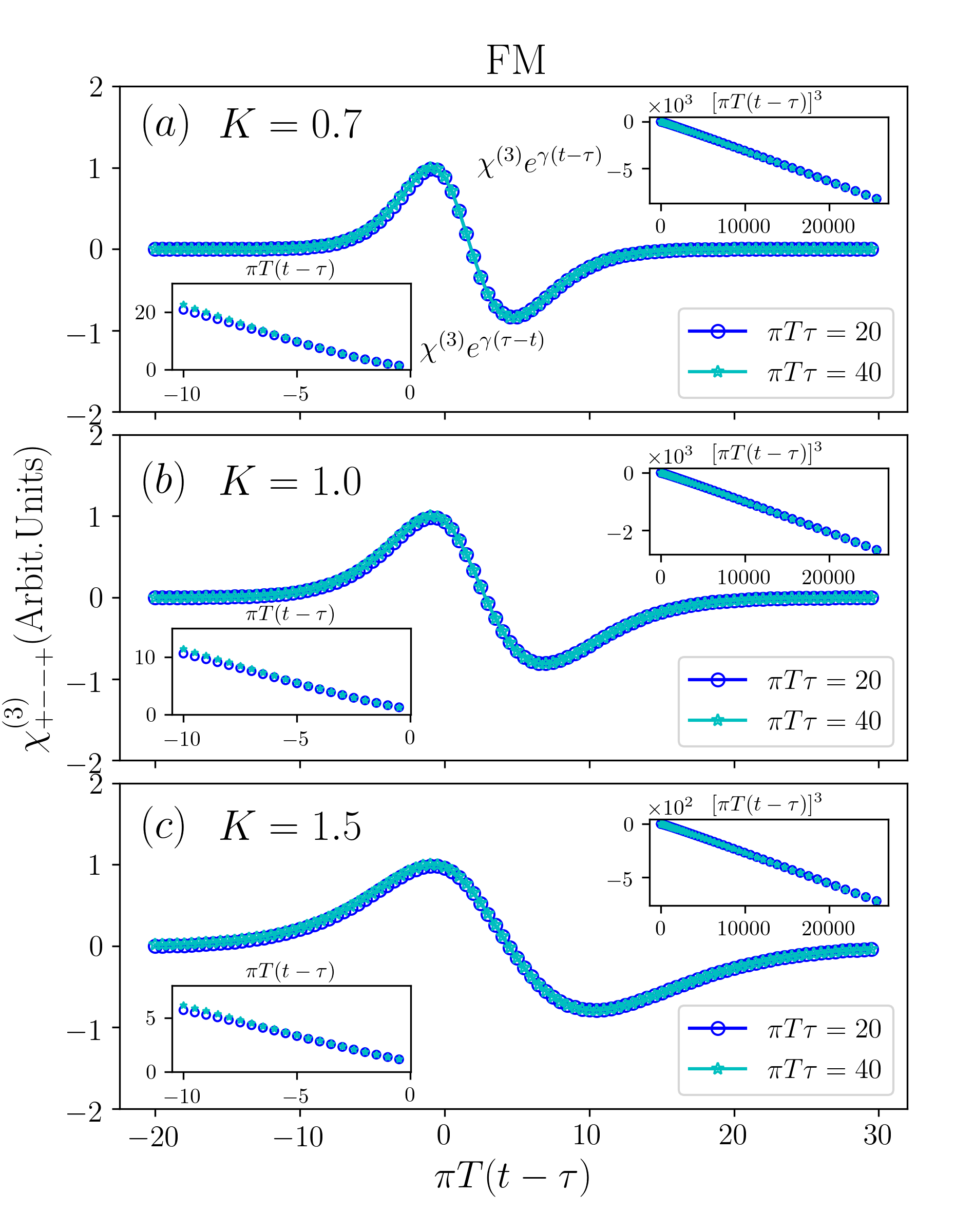
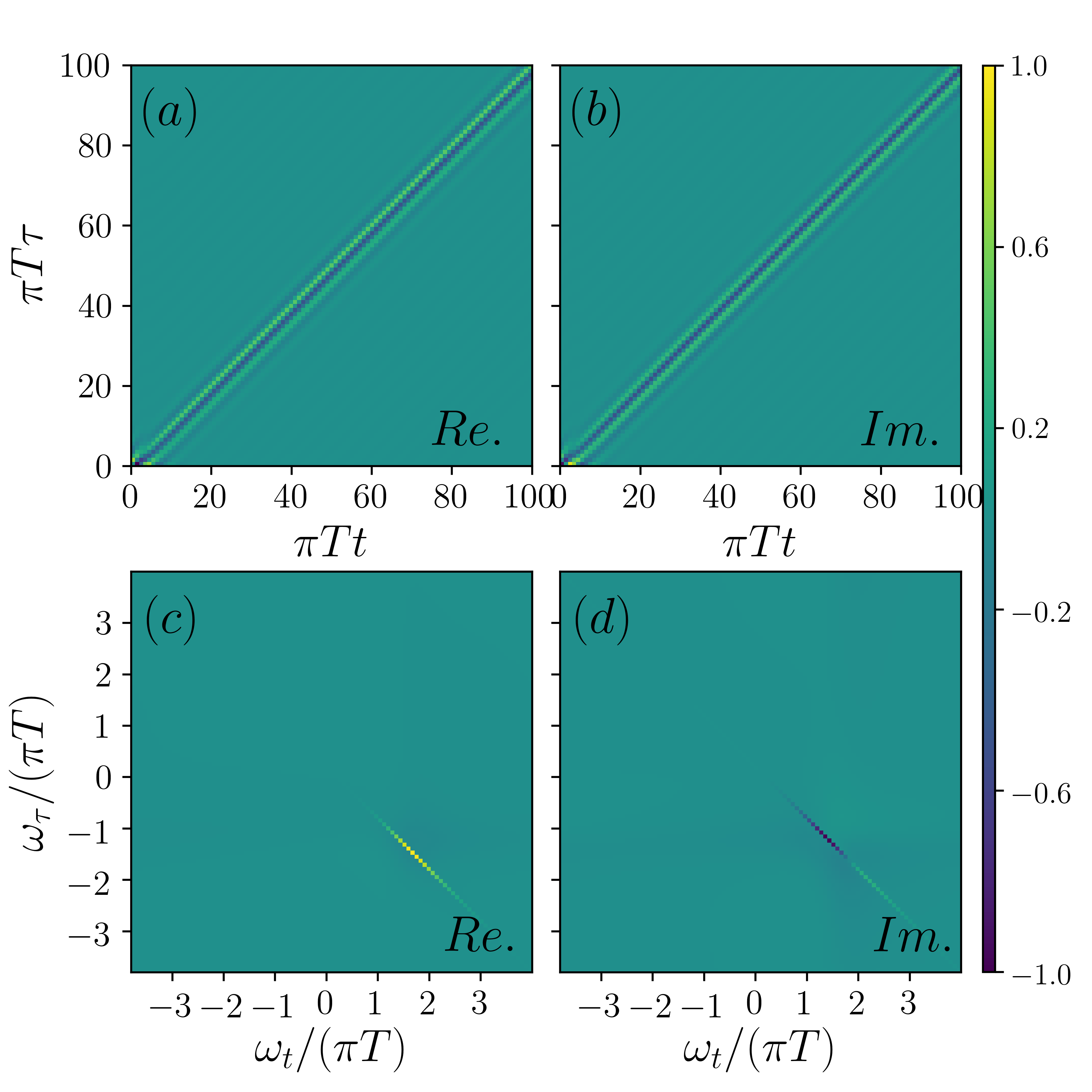
Fig. 2 shows for representative Luttinger parameters , , and . and . For all cases, the nonlinear response shows a surge near , exhibiting the clear signature of photon echo. Note the maximum is not exactly located at but fairly close to it. The data for different values of overlay within numerical error when plotted as a function of . This demonstrates the photon echo is independent of for large .
Numerical integration also indicates that the value of measured at does not depend on within numerical error in the asymptotic regime , which is in agreement with Eq. (19)
We further examine the asymptotic behavior of by multiplying it with . Eq. (19) suggests the product would be when , and when . The insets of Fig. 2 show that its behavior is in excellent agreement with Eq. (19).
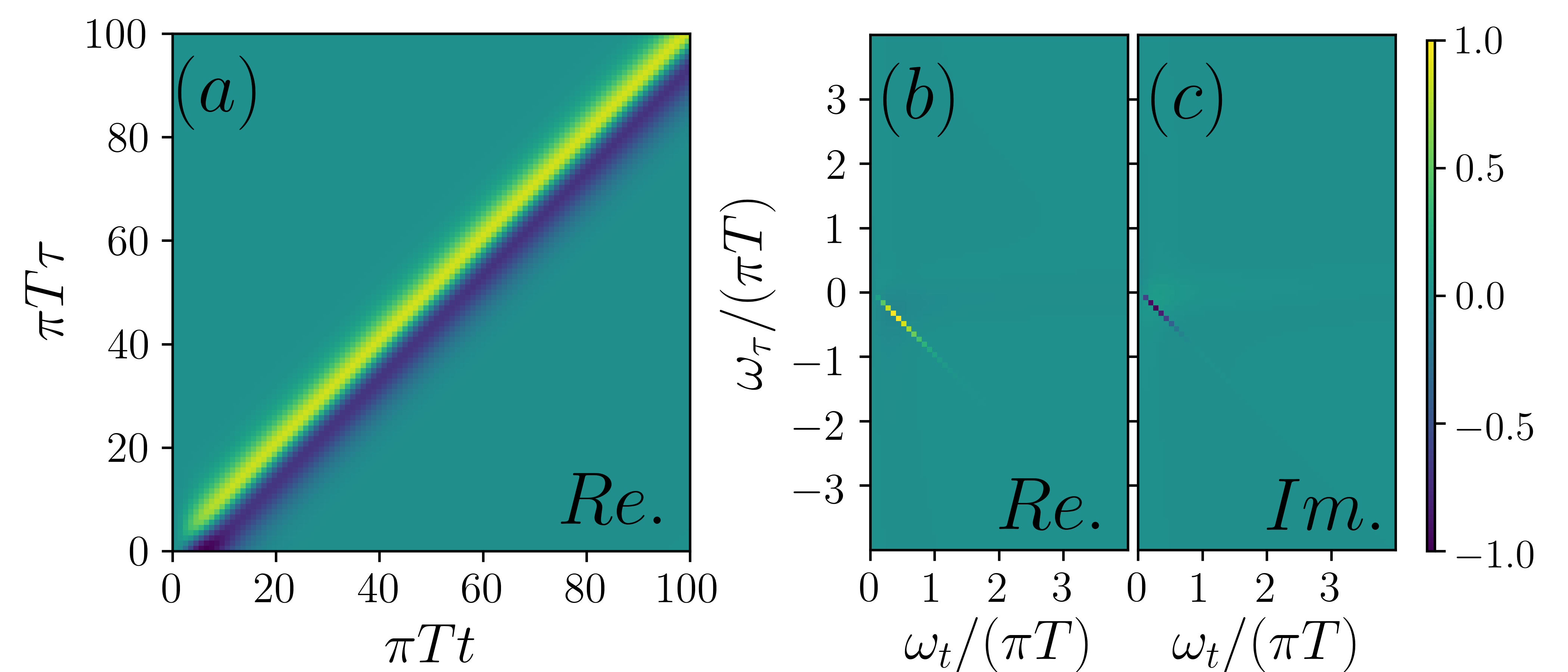
Having analyzed the photon echo signal for fixed value of , we now scan and present the nonlinear response as a function of both and . Fig. 3(a) shows for and . The photon echo appears as a bright feature at the diagonal of the plane. This feature persists along the diagonal direction, highlighting the fact that the photon echo is perfect.
Performing the FFT of the time domain data yields the two-dimensional spectrum (Fig. 3(b)&(c)). In the frequency domain, the photon echo manifest itself as a pair of highly anisotropic peaks in the second/fourth quadrants, symmetrically distributed with respect to the origin. The peak width along the diagonal direction of the second/fourth quadrant scales with . The peak width along the anti-diagonal direction is resolution limited — the photon echo signal in the time domain (Fig. 3(a)) is independent of at late time, and hence its Fourier transform .
To recapitulate, the of the ferromagnetic chain is real and independent of the magnetization density. It exhibits perfect photon echo, which depends on rather than and both.
III.4 AFM chain
We turn to the antiferromagnetic () case in this subsection. We write the spin operator as:
| (20) |
where we have defined vertex operators and for later convenience. Inserting the above into Eq. (9) yields:
| (21) |
We have defined a set of response functions with the form of Eq. (10). For instance, is defined as:
| (22) |
The other response functions are defined in the same vein. The expression for these response function can be read off from Eq. (13) by plugging in appropriate values of and : and for vertex operator ; for vertex operator , the value of and are switched. We have dropped the response functions that violate the charge neutrality condition (e.g. ) as they vanish in the thermodynamic limit.
The calculation of parallels the ferromagnetic case (Sec. III.3). Note, however, is now complex and depends on the magnetic field through the magnetization density . We find only and contribute to photon echo. Using the approximation (Eq. (16)), we obtain after lengthy calculation:
| (25) |
Here, we have defined a parameter . The above is the key result of this subsection.
Eq. (25) shows that the of antiferromagnetic chain exhibits perfect photon echo similar to the ferromagnetic chain. Different from the ferromagnetic chain, the signal now shows oscillations with the frequency set by the magnetization density , which, in turn, depends on the magnetic field . The time scale of the signal is . In particular, in the Heisenberg limit where (), the time scale diverges — this reflects the Larmor precession of the total magnetization, which we elaborate on in Appendix C.
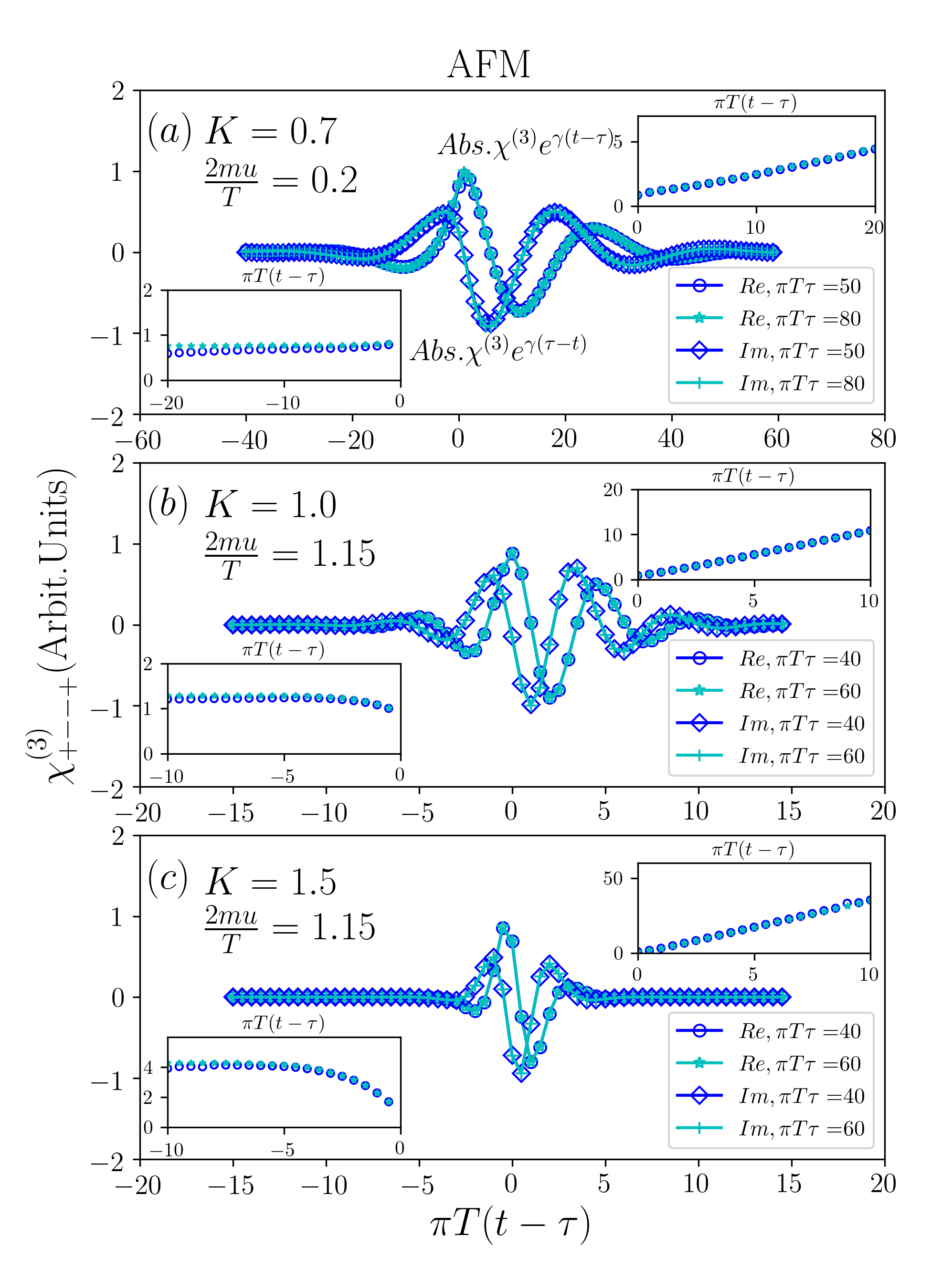
We assess the validity of Eq. (25) by numerical integration. Fig. 4 show for representative Luttinger parameters , , and . . The echo is clearly visible from the data. The data for different values of overlay when plotted as a function of , demonstrating that the echo is perfect. Numerical integration suggests is independent of within numerical error when and are large.
To test the asymptotic behavior of , we multiply its complex modulus with . Eq. (25) suggests the product shows linear behavior for and approaches a constant for . The insets of Fig. 4 show good agreement with Eq. (25). For and , the data deviate slightly from the constant behavior; we think this occurs because is not sufficiently large to suppress the non-asymptotic contributions.
We then present the dependence of the photon echo signal on both and . Fig. 5(a)&(b) show the real and imaginary parts of as a function of and for the Luttinger parameter . The magnetization density . The waiting time . The photon echo appears as the bright feature persists along the diagonal direction (). Performing Fourier transform over and produces the two-dimensional spectrum (Fig. 5(c)&(d)). The photon echo appears in the frequency domain as a highly anisotropic peak in the fourth quadrant. The peak is approximately located at and as suggested by Eq. (25). Its width along the diagonal of the fourth quadrant scales with , whereas its width along the anti-diagonal direction is resolution limited.
To recapitulate, the of the antiferromagnetic chain shows clear signature of perfect photon echo. The echo signal is oscillatory with the frequency set by magnetization density.
IV Spinon Lensing Picture
In the previous section, we have shown that the nonlinear magnetic susceptibility of the Luttinger spin liquid exhibits photon echo that resembles the perfectly rephasing echo in a few-body system such as a single spin. In this section, we provide an intuitive picture that clarifies its origin in the many-body system under consideration, namely Luttinger spin liquids. We illustrate our picture on the ferromagnetic spin chain and then generalize it to the antiferromagnetic chain, and discuss its various features and implications.
To set the stage, we review the effect of the bosonized spin raising operator . Let us consider the time evolution after the operator at on the initial state at which is assumed to be an energy eigenstate. At time , the state is given by
| (26) |
where we used the assumption that is an energy eigenstate and dropped the overall phase factor. We can decompose the field to chiral components as
| (27) |
where
| (28) |
The equation of motion implies that each chiral components depends only on the corresponding light cone coordinate, as in Eq. (27). Using this, we can translate the time dependence into the position dependence, so that
| (29) |
where is now understood as a static operator at locations , up to the overall phase factor which includes the one coming from the commutation relation between and .
Now, recall the equal-time commutation relation:
| (30) |
Namely, creates a kink of step in -field at the location . Since this step corresponds to the magnetization density , this kink can be interpreted as a spinon [17]. Eq. (29) then implies that the application of the operator at is equivalent to creation of a right-moving spinon at and a left-moving spinon at at time , when the other operations are applied after the time . The chiral vertex operators can be viewed as spinon creation operators of the corresponding chirality. This justifies the following simple visual picture: Applying creates a pair of the right-moving and left-moving spinons at . Then these spinons propagate with the constant velocity .
Real-time correlation functions of the vertex operators can be qualitatively understood in terms of this visual picture. As the simplest example, consider the two-point correlation function (Fig. 6a)
| (31) |
Here, we set and omit an overall phase factor. This correlation function corresponds to the creation of a pair of spinons at , and the annihilation of a pair of spinons (or equivalently the creation of a pair of anti-spinons) at the origin. From the equation of motion (the second line), this correlation function can be interpreted as an expectation value of spinon creation operators at the split locations and two spinon annihilation operators at . For a generic choice of , these three locations are different. As a result, the expectation value, although does not vanish completely, is exponentially suppressed with respect to the correlation length at finite temperature .
If we wish to maximize the correlation function, we should try to “catch” the spinons created at at the later time and annihilate them. If we can manage to annihilate all the spinons created earlier, the correlation function would be reduced to the equal-time correlation function of the identity operator, which does not decay as a function of time at all! Unfortunately, it is impossible to annihilate both spinons created at by the single operator , since spinons split and are located on different positions at later times.
We note it is possible to annihilate one of them, for example the left-moving spinon, by choosing the location of the second operator on the left side of the light cone (, or ). Setting in Eq. (31) maximizes the first factor, which is formally divergent in the scaling limit (the cutoff ) but bounded to be a finite constant due to the finite in a realistic system. However, implies , leading to the exponential suppression of the other factor in Eq. (31). Thus the two-point correlation function is exponentially suppressed for large , for any choice of the relative spatial location .
The situation is quite different for four-point correlation functions and corresponding response functions. It is convenient to rewrite the response function Eq. (15) as a sum over various four-point correlation functions by expanding the nested commutators:
| (32a) | ||||
| where | ||||
| (32b) | ||||
| (32c) | ||||
| (32d) | ||||
| (32e) | ||||
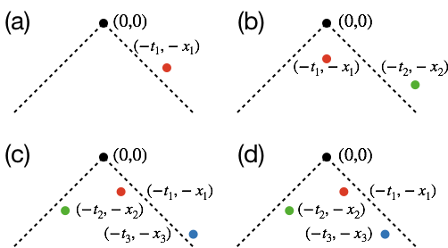
is related to by reversing the order of operators in the product. Following Ref. 1, 2, each contribution can be identified as a Liouville pathway.
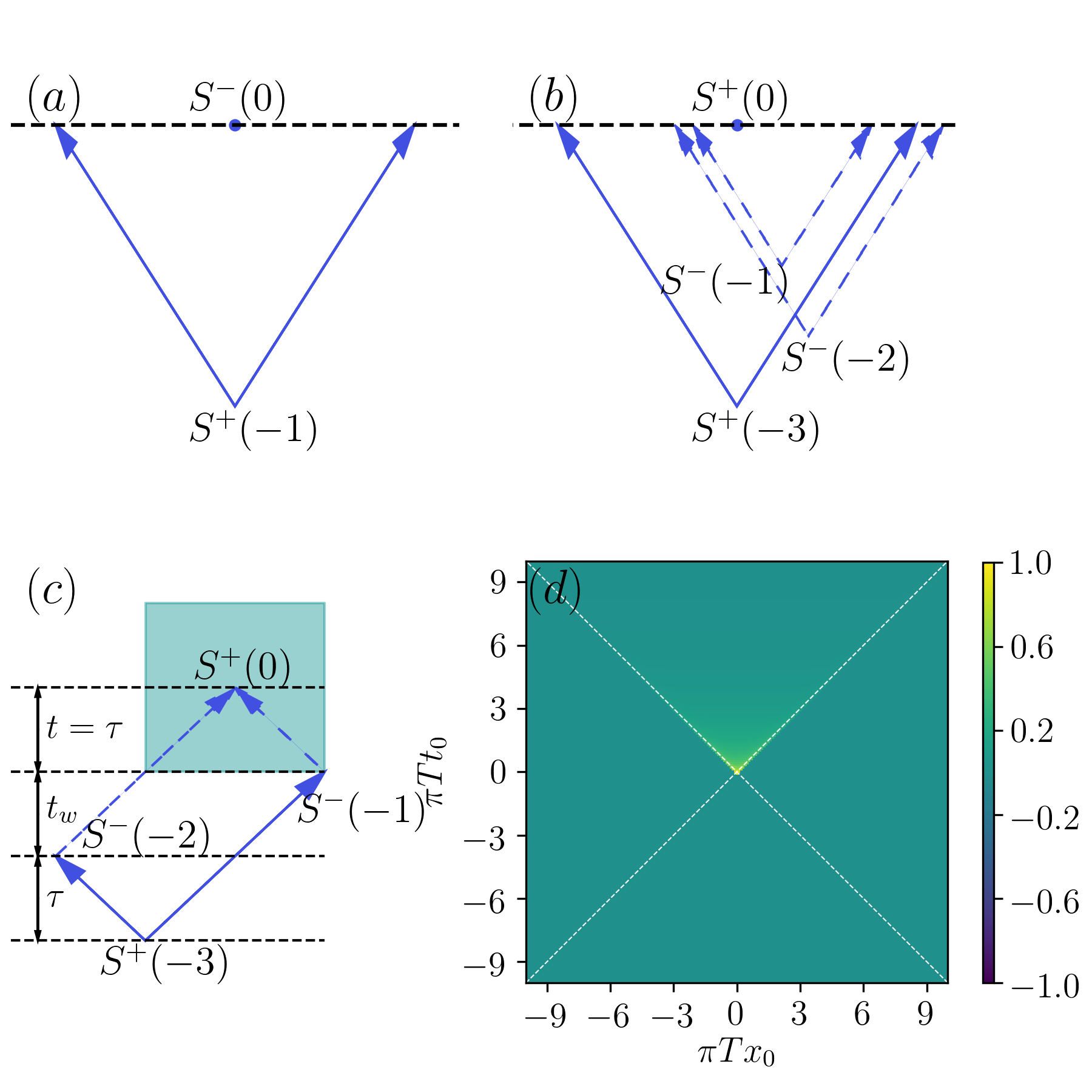
We find that each four-point correlation function can be made free from exponential suppression for an appropriate choice of locations of the operators at given set of times. As exchanging the order of operators in only results in a phase factor, it is sufficient for our purpose to consider the correlation function (Fig. 6b). The spinon pairs are created at and , and annihilated at and . Unlike the case with the two-point correlation function (Eq. 31), here, we can catch and annihilate all the spinons created earlier by choosing (Fig. 6c):
| (33) |
For this configuration, the operator at annihilates the left-moving spinon created at and creates a right-moving antispinon. The operator at annihilates the right-moving spinon created at and creates a left-moving antispinon. The two antispinons moving to the opposite directions finally meet at the origin at time , and are annihilated by the operator ! As a consequence, the magnitude of the four-point correlation function reaches its maximum and does not decay even in the long-time limit as long as the spatial coordinates are chosen according to Eq. (33). We call this phenomenon, which was absent in the two-point correlation function, the spinon lensing, that is, it is possible to focus the two (anti)spinons to the same point at time , by placing the operators judiciously at earlier times. We also note that the spatial mirror reflection of Eq. (33) is equally valid for lensing.
The above reasoning can be made precise by applying the equation motion to reduce the -point correlation function to an equal-time correlation function at time of multiple operators — spinon creation operators at locations and two at , and antispinon creation operators at locations and (Fig. 6b). Under the condition Eq. (33), the locations of the spinon creation operators match with those of the spinon annihilation operators, and consequently the correlation function reaches the maximum.
The same phenomena occur in the other four-point correlation functions. Summing them up, the nonlinear response as a function of spacetime coordinates , , and , reaches a maximum at the lensing configuration Eq. (33). Fig. 6d shows the behavior of as a function of the detection position in a representative lensing configuration. Here we choose and . It shows that the response is maximum at the “focal point” . As we have used a finite short distance cutoff to regularize the algebraic singularity at the light cone, we have slightly shifted and away from the light cone by a small distance to suppress the effect of the regularizer.
Now, the optical nonlinear response is related to by spatial integration. When the time delays , the spatial integration is dominated by the neighborhood of the lensing configuration Eq. (33) and its mirror reflection, and, as a result, remains non-vanishing even in the long-time limit . This explains the origin of the prefect photon echo observed in the of the ferromagnetic chain.
Turning to the antiferromagnetic chain, is now a linear combination of various four-point response functions (Eq. (21)). Among these, and support the lensing phenonenon similar to Fig. 6 with the only difference being the type of fractional excitations created/annihilated by the spin operators. In the antiferromagnetic chain, creates a pair of spinons plus a pair of Laughlin quasiparticle and quasihole [17]. Note the created spinon and the Laughlin quasiparticle (and similarly the created antispinon and the Laughlin quasihole) are superimposed on each other, and therefore the world lines shown in Fig. 6 should be interpreted as the world line of the composite object. Our numerical calculations show that, indeed, only these two response functions produce photon echo whereas the others response functions do not.
In Sec. II, we have pointed out that the nonlinear susceptibilities and do not exhibit photon echo. This can now be easily understood in terms of lensing. For these two susceptibilities, it is impossible to arrange the spin operators in such a way that all the created fractional excitations get annihilated at a later time. Our calculations indeed confirm this.
Our discussion so far is based on the ideal Luttinger spin liquid at the RG fixed point. In general, there are RG-irrelevant perturbations to the fixed point Hamiltonian Eq. (3), but they only give sub-leading corrections to most of the physical quantities at low temperatures. This also makes these RG-irrelevant corrections difficult to detect in experiments. Nevertheless, in the 2DCS in Luttinger spin liquid, the RG-irrelevant perturbations can produce pronounced effects because the lensing of fractional excitations relies on two features of the fixed point Hamiltonian: First, the phonon modes are the exact eigenstates of the Hamiltonian. Second, the phonon dispersion relation is exactly linear. These features ensure that a wave packet of fractional excitation can propagate indefinitely through the system without dissipation or dispersion. RG-irrelevant corrections to the fixed point Hamiltonian would prevent the indefinite propagation of the wave packet, and, therefore, could be sensitively detected by the suppression of lensing.
In the XXZ spin chain, the RG-irrelevant perturbations include the umklapp terms such as [15, 16], which result in the damping of phonon modes at finite temperature. Consequently, the wave packets of fractional excitations acquire finite life time. The lensing phenomenon shown in Fig. 6 is suppressed when or exceeds the life time of these excitations. This, in turn, will be manifest as the decay of the photon echo signal as or increases, in close analogy with the dissipation-induced photon echo decay in few-body systems [1, 2]. Straightforward dimensional analysis suggests the decay rate vanishes as as where is the dimension of the umklapp term.
On the other hand, there also exist a different family of RG-irrelevant perturbations, such as , which produce a small curvature in the phonon dispersion relation while keeping them as the exact eigenstates of the Hamiltonian. As a result, the wave packet disperses as it propagates, but there is no true dissipation. The lensing picture suggests that the dispersion of wave packet would also result in the decay of the photon echo. For instance, the wave packet of the left-moving spinon created by would be quite dispersed when is large. It could not completely annihilate with the left-moving antispinon created by as the latter’s wave packet is still sharp. This would spoil lensing. Thus, the lensing picture suggests a dispersion-induced decay mechanism for the photon echo in the Luttinger spin liquid. In the next section, we examine this mechanism in more detail.
V Dispersion-induced decay
The spinon lensing picture suggests that the dispersion of the wave packets could also lead to the decay of photon echo. In this section, we put this idea to test by a numerical experiment. We consider the harmonic chain, which is a discretization of the fixed point Hamiltonian:
| (34) |
Here, is the lattice constant. resides on the lattice site labeled by , whereas resides on the midpoint of the lattice link connecting the site and . Their commutation relation is given by: . It is sufficient for our purpose to consider the ferromagnetic chain where . We set the Luttinger parameter .
The phonon modes are exact eigenstates of Eq. (34) owing to its quadratic form. The phonon dispersion relation is now nonlinear: . Therefore, Eq. (34) represents an idealized model system to study the dispersion-induced decay without the complications of dissipation effects. By contrast, in a microscopic spin lattice model, both effects are present and difficult to disentangle.
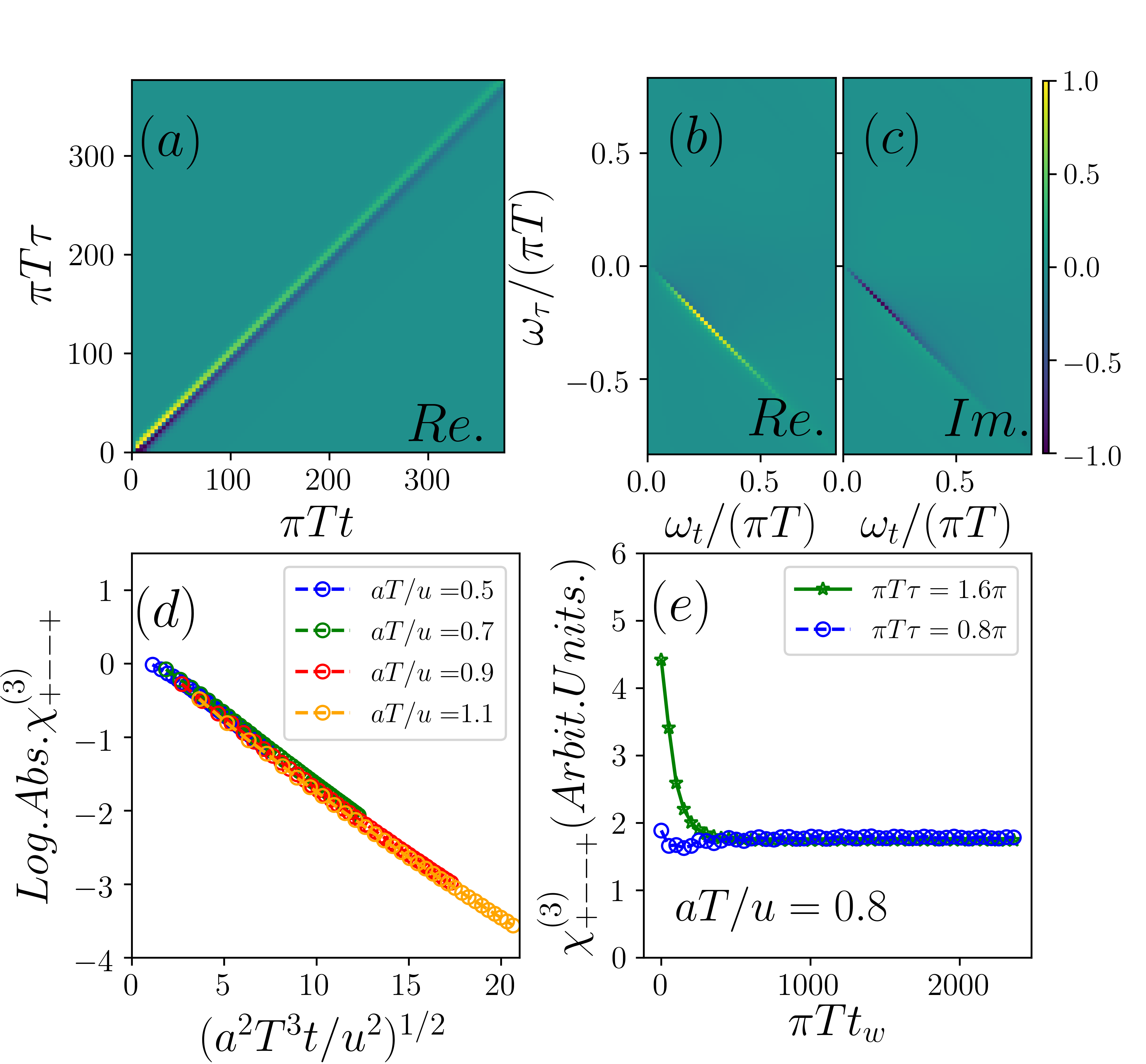
Fig. 7(a) shows as a function of and at temperature . The waiting time . Note the data are strictly real as the case in continuum (Fig. 3). We find a clear signature of photon echo running along the diagonal of the plane. However, the echo signal decays slowly along the diagonal direction owing to the dispersion effect. In the frequency domain, this decay manifests itself as a slight broadening of the photon echo peaks along the anti-diagonal direction of the frequency plane (Fig. 7(b)&(c)).
We now investigate the temperature dependence of the dispersion-induced decay. Expanding the phonon dispersion near , we obtain . Therefore, the width of the wave packet grows as as it propagates. At temperature , this defines a dispersion time scale :
| (35) |
Here, is the spin correlation length. Beyond this time scale, the wave packet is essentially indistinguishable from thermal fluctuations. Thus, we hypothesize that the decay of the echo signal is controlled by .
Our data support this hypothesis. Fig. 7(c) shows the semi-log plot of at as a function of . The data for different approximately collapse to a straight line. This suggests the echo signal decays as a stretched exponential, , where the exponent and is a numeric constant. The decay rate , consistent with the dimension of the higher derivative term . The origin of the stretching exponent is unclear at the moment but likely associated with the asymptotic behavior of Airy functions.
Having investigated the decay of the echo as a function of , we turn to its dependence. Fig. 7(e) shows at as a function of for two representative values of . The echo signal initially decrease as increases, reflecting the effect of dispersion, but eventually saturate to a finite value This is also consistent with the lensing picture. A straightforward calculation shows that the spacetime-dependent susceptibility saturates to finite value as at the lensing configuration Eq. (33). In a few-body system, the decay of photon echo as a function of reflects the thermal relaxation of the optical population. Here, as the phonon modes are exact eigenstates of the Hamiltonian Eq. (34), the phonon population cannot relax. We therefore heuristically attribute the saturation to the absence of thermal relaxation in Eq. (34).
To recapitulate, by a numerical experiment, we have shown that the photon echo signal decays as a function of in the presence of wave packet dispersion. The decay is controlled by a dispersion time scale . Meanwhile, the echo signal saturates as , which we attribute to the lack of thermalization in the model system.
VI Discussion
In this work, we have shown that the nonlinear magnetic susceptibility and its complex conjugate of the Luttinger spin liquid exhibit photon echo that resembles the perfectly rephasing photon echo in a few-body problem. However, the rephasing picture does not directly apply to the present system in that its energy spectrum is continuous. Instead, the echo signal arises from the lensing of the fractional excitations, and its decay as a function of the pulse delays is a sensitive diagnostic for the dissipation and/or dispersion.
The photon echo can be directly measured by THz 2DCS on spin chain materials that host Luttinger spin liquids. For example, Cs2CoCl4 is thought to be a realization of the easy-plane antiferromagnetic () XXZ chain [23]. Although our analysis is carried out in the circular polarization basis, one could simplify the experimental set up by measuring the response with linear polarization (e.g. ) since the linear polarization basis and the circular polarization basis are related by a linear transformation.
We find the lensing of fractional excitations to be a convenient picture for understanding the photon echo in the Luttinger spin liquid. A crucial feature of the lensing is the refocusing of the wave packets world lines, reminiscent of the refocusing of quantum phase accumulation in the NMR spin echo or photon echo in few-body systems. However, the lensing is unique to many-body system in that it entails the propagation of wave packets. It could be viewed as a conceptual extension of the more familiar interference picture [1, 2] commonly used in the study of photon echo in few-body systems from the time domain to the spacetime domain.
An earlier work on the photon echo of quantum Ising chain uses the time-domain interference picture [7], which is made possible by a mathematical mapping that relates the nonlinear response of a many-body system to that of an ensemble of independent few-body systems. Although it might be possible to adapt this methodology for the Luttinger spin liquid, we think it will be much less illuminating given the complex structure of the optical matrix elements.
An interesting consequence of the lensing picture is that the dispersion of the wave packet alone could lead to the decay of photon echo signal. This decay mechanism finds no immediate analogue in few-body systems. In the presence of dispersion but no dissipation, the echo signal decays as increases and eventually disappears when far exceeds the dispersion time scale. However, the echo signal does not disappear when the waiting time . This points toward different uses of the pulse delays and — the former could be used as a dial to monitor both dispersion and dissipation effects, whereas the latter is sensitive to dissipation alone.
Our work opens a few directions worth further investigation. First of all, our discussion on the umklapp terms, or more broadly dissipation effects, has been qualitative. It will be useful to examine their impact on the photon echo quantitatively by employing the quantum kinetic theory [24, 25]. Secondly, it would be interesting to compare our predictions with lattice model calculations. Our preliminary results on the XY spin chain [26, 27, 28, 29, 30] show good agreement with the bosonization predictions and will be published elsewhere. Thirdly, our analysis focuses on the gapless phase of the XXZ type spin chain. It would be interesting to explore the nonlinear photon echo in the gapped phase by using a semiclassical treatment [31, 32, 33], or in the vicinity of the Heisenberg point where the proximate symmetry might gives rise to new universal features [34, 35]. We also note an interesting recent work where the generalized hydrodynamics is employed to compute some nonlinear responses of integrable systems including the XXZ spin chain [36]. Finally, even though we exclusively consider the spatially uniform (momentum ) magnetic response in this work, our calculations can be generalized to finite . It has been shown that, in a magnetized antiferromagnetic Heisenberg chain, the magnetic resonance mode acquires a nonlinear dispersion at due to spinon interactions [37, 38]. In light of these results, we expect that the nonlinear magnetic resonance may exhibit rich physics. Although optical measurements usually probes the response, the presence of Dzyaloshinskii-Moriya (DM) interaction in a spin chain may allow for optical measurement of the responses. The DM interaction may be eliminated by a gauge transformation at the expense of a momentum boost [39]. Hence, the response of the spin chain with a uniform DM interaction is equivalent to the finite response of the corresponding spin chain without the DM interaction [40, 41].
Looking beyond the Luttinger spin liquids, we think our method and the physical picture could be applicable to other one-dimensional critical systems and potentially higher dimensional systems. Perhaps the most experimentally relevant are gapless systems with charged excitations, where the charge degrees of freedom could directly couple to the electric component of the THz pulse and therefore produce stronger nonlinear response. In short, we believe future investigation on the nonlinear response of many-body systems will uncover far richer dynamical phenomena and offer deeper insight into these systems.
Acknowledgements.
YW and MO thank the hospitality of the Kavli Institute for Theoretical Physics, University of California, Santa Barbara, where a part of this work was performed. MO also thanks Shunsuke Furukawa, Shunsuke C. Furuya, and Masahiro Sato for useful comments. This work was supported in part by the National Natural Science Foundation of China (Grant No. 11974396), the Strategic Priority Research Program of the Chinese Academy of Sciences (Grant No. XDB33020300), Japan Society for the Promotion of Science (Grant Nos. JP18H03686 and JP19H01808), Japan Science and Technology Agency CREST (Grant No. JPMJCR19T2), and the National Science Foundation (Grant No. NSF PHY-1748958). A part of the numerical calculations were carried out on Tianhe-1A at the National Supercomputing Center in Tianjin, China.Appendix A Commutation relation prescriptions
In this appendix, we discuss the different choices for the commutation relation between and fields, and the subtle issues [42] associated with these choices. Although elementary, these issues are pertinent to the calculation of higher order response functions.
In bosonization, and form a pair of canonical conjugate variables:
| (36) |
The above does not uniquely fix the commutator between and . Several popular choices exist in literature. In this work, we use:
| (37) |
We term this choice the “Heaviside prescription” for latter convenience. A closely related variant is [15]. Since the two variants are rather similar, we shall focus the prescription Eq. (37). Another popular choice is [16]:
| (38) |
We term this choice the “signum prescription”.
In what follows, we show that the different prescriptions result in different bosonization dictionaries. We first consider the fermion field operator. For non-interacting fermions (Luttinger parameter ), the left and right chiral boson fields are dynamically coupled:
| (39) |
The commutation relation of , and likewise , are identical for both prescriptions. However, the commutator between and depends on the prescription:
| (42) |
In other words, boson fields with different chiralities do not commute (commute) in the Heaviside (signum) prescription. As a result, in the Heaviside prescription, the left and right chiral fermions:
| (43a) | |||
| anti-commute thanks to the commutator between and . By contrast, in the signum prescription, Klein factors are needed to ensure the anti-commutation relation: | |||
| (43b) | |||
where are the Klein factors obeying the Clifford algebra: , and .
It is important to bear in mind that choosing different prescriptions do not change the dynamics of the boson fields. Furthermore, including fermion interactions () does not spoil the commutator between the left and right chiral boson fields. In this case, the two dynamically decoupled fields read:
| (44) |
and we find Eq. (42) holds regardless the value of .
In the next, we consider the Jordan-Wigner string operator, which plays a crucial role in the bosonization of the XXZ spin chain:
| (45) |
where is the fermion annihilation operator on lattice site . In particular,
| (46) |
We now bosonize the string operator following the standard procedure [15, 16]:
| (47) |
In the Heaviside prescription, the boundary term commutes with . We thus may regard it as a number and omit it:
| (48a) | |||
| By contrast, in the signum prescription, we must keep the boundary term as : | |||
| (48b) | |||
In the signum prescription, the boundary term is needed to reproduce the commutation relation between the fermion field operator and the string operator (Eq. 46). Had we dropped the boundary term, we would have found:
| (49) |
which disagrees with Eq. 46.
Finally, we are ready to bosonize the spin operators of the XXZ chain using the bosonization expressions of the fermion operator and the string operator. We assume the chain is antiferromagnetic () without loss of generality. Following Refs. 15, 16 but keeping a close eye on the Klein factors and the boundary term, we find the staggered components of the spin operators are given by:
| (52) |
| (55) |
We stress that the Klein factors and the boundary term are essential in reproducing the correct commutation relations. For instance, had we dropped the Klein factors and the boundary term, we would have obtained:
| (56) |
using the signum prescription. This is incorrect because these two operators must commute.
For the uniform components, we have:
| (57) |
which is independent of the prescription, and
| (60) |
We see that the bosonization dictionary takes a much simpler form in the Heaviside prescription. In fact, the Heaviside prescription has been used in the literature [43, 44] when the precise bosonization formulae are needed. On the other hand, the full bosonization formulae of the spin operators in the chain in the signum prescription given in Eqs. (52), (55), and (60) are new to the best of our knowledge. For the signum prescription, one might hope that we could omit the Klein factors and the boundary term in calculations and still get correct results. This is indeed the case when calculating two-point functions, which is a fortunate coincidence. In fact, dropping the Klein factors and the boundary term from the bosonization dictionary can lead to incorrect results in the signum prescription when calculating higher order response functions.
To illustrate this point, consider the following four-point response function:
| (61) |
Had we dropped the Klein factors and the boundary term in the Signum prescription, we would have found and anti-commute when they are spacelike separated (Eq. (56)). As a result, even when the point of detection is outside the light cone of the perturbation, thereby violating the causality principle.
To recapitulate, different choices for the commutation relation of and lead to different bosonization dictionaries. The bosonization dictionary in the signum prescription includes Klein factors and the boundary term, which cannot be omitted in calculating the high-order response functions.
Appendix B Causality of the response function
In this appendix, we prove the causality of the response function (Eq. (10)).
To set the stage, we recall that causality in relativistic quantum field theory requires that two observables commute if their separation is spacelike:
| (62) |
where are arbitrary observables.
We first prove the following general statement: is causal provided that all the operators that appear in Eq. (10) fulfil the condition Eq. (62). Specifically, we need to show if any of the three spacetime points , , are outside the light cone of . We prove this statement by exhaustion:
- (i)
- (ii)
- (iii)
This completes our proof.
In the next, we turn to the Tomonaga-Luttinger liquid theory and show that the local vertex operators:
| (63) |
indeed fulfill the condition Eq. (62). To this end, we consider two vertex operators and . Suppose they are spacelike separated. We choose a reference frame in which they are synchronous and compute their equal time commutator:
| (64) |
The second equality follows from the Baker-Campbell-Hausdorff formula; the third equality follows from the fact . The above immediately implies:
| (65) |
Thus, we have verified that the local vertex operators fulfill the causality condition Eq. (62).
Appendix C Antiferromagnetic Heisenberg chain
In this appendix, we compute of the antiferromagnetic Heisenberg chain ( in Eq. (1)) by using the equation of motion of the lattice model [34, 35].
The equation of motion for the total magnetization reads:
| (66) |
The second equality follows from the fact that the Heisenberg interaction, being symmetric, commutes with . Solving the above, we find:
| (67) |
Substituting the above into the Kubo formula for , and using the spin commutation relation, we obtain:
| (68) |
where is the magnetization density. Therefore, for the Heisenberg chain, the nonlinear magnetic susceptibility shows oscillation with constant magnitude, which reflects the Larmor precession of the total magnetization vector. We stress that this simplicity is unique to the spatially uniform (momentum ) response function. By contrast, the magnetic response functions may exhibit rich physics that is beyond the Larmor precession. For instance, the dispersion relation of the magnetic resonance mode, emanating from the Larmor frequency at , acquires a curvature thanks to the spinon interactions [37, 38]. These effects are not visible in the response function.
References
- Mukamel [1995] S. Mukamel, Principles of Nonlinear Optical Spectroscopy (Oxford University Press, Oxford, 1995).
- Hamm and Zanni [2011] P. Hamm and M. Zanni, Concepts and Methods of 2D Infrared Spectroscopy (Cambridge University Press, Cambridge, 2011).
- Cundiff and Mukamel [2013] S. Cundiff and S. Mukamel, Optical multidimensional coherent spectroscopy, Physics Today 66, 44 (2013).
- Woerner et al. [2013] M. Woerner, W. Kuehn, P. Bowlan, K. Reimann, and T. Elsaesser, Ultrafast two-dimensional terahertz spectroscopy of elementary excitations in solids, New Journal of Physics 15, 025039 (2013).
- Lu et al. [2017] J. Lu, X. Li, H. Y. Hwang, B. K. Ofori-Okai, T. Kurihara, T. Suemoto, and K. A. Nelson, Coherent Two-Dimensional Terahertz Magnetic Resonance Spectroscopy of Collective Spin Waves, Phys. Rev. Lett. 118, 207204 (2017).
- Mahmood et al. [2020] F. Mahmood, D. Chaudhuri, S. Gopalakrishnan, R. Nandkishore, and N. P. Armitage, Observation of a marginal Fermi glass using THz 2D coherent spectroscopy (2020), arXiv:2005.10822 [cond-mat.str-el] .
- Wan and Armitage [2019] Y. Wan and N. P. Armitage, Resolving Continua of Fractional Excitations by Spinon Echo in THz 2D Coherent Spectroscopy, Phys. Rev. Lett. 122, 257401 (2019).
- Choi et al. [2020] W. Choi, K. H. Lee, and Y. B. Kim, Theory of Two-Dimensional Nonlinear Spectroscopy for the Kitaev Spin Liquid, Phys. Rev. Lett. 124, 117205 (2020).
- Parameswaran and Gopalakrishnan [2020] S. A. Parameswaran and S. Gopalakrishnan, Asymptotically exact theory for nonlinear spectroscopy of random quantum magnets, Phys. Rev. Lett. 125, 237601 (2020).
- Nandkishore et al. [2020] R. M. Nandkishore, W. Choi, and Y. B. Kim, Spectroscopic fingerprints of gapped quantum spin liquids, both conventional and fractonic (2020), arXiv:2010.07947 [cond-mat.str-el] .
- Phuc and Trung [2020] N. T. Phuc and P. Q. Trung, Direct and ultrafast probing of quantum many-body interaction and mott-insulator transition through coherent two-dimensional spectroscopy (2020), arXiv:2009.08598 [cond-mat.str-el] .
- Kurnit et al. [1964] N. A. Kurnit, I. D. Abella, and S. R. Hartmann, Observation of a Photon Echo, Phys. Rev. Lett. 13, 567 (1964).
- Hahn [1950] E. L. Hahn, Spin Echoes, Phys. Rev. 80, 580 (1950).
- Babujian et al. [2016] H. M. Babujian, M. Karowski, and A. M. Tsvelik, Probing strong correlations with light scattering: Example of the quantum Ising model, Phys. Rev. B 94, 155156 (2016).
- Affleck [1988] I. Affleck, Field theory methods and quantum critcal phenomena, in Les Houches Summer School in Theoretical Physics: Fields, Strings, Critical Phenomena (1988) pp. 563–640.
- Giamarchi [2003] T. Giamarchi, Quantum Physics in One Dimension (Oxford University Press, Oxford, 2003).
- Pham et al. [2000] K.-V. Pham, M. Gabay, and P. Lederer, Fractional excitations in the luttinger liquid, Phys. Rev. B 61, 16397 (2000).
- Zvezdin and Kotov [1997] A. Zvezdin and V. Kotov, Modern Magnetooptics and Magnetooptical Materials (Taylor & Francis, New York, 1997).
- Boyd [2008] R. Boyd, Nonlinear Optics, 3rd ed. (Academic Press, Cambridge, Massachusetts, 2008).
- Luther and Peschel [1975] A. Luther and I. Peschel, Calculation of critical exponents in two dimensions from quantum field theory in one dimension, Phys. Rev. B 12, 3908 (1975).
- Haldane [1980] F. D. M. Haldane, General Relation of Correlation Exponents and Spectral Properties of One-Dimensional Fermi Systems: Application to the Anisotropic Heisenberg Chain, Phys. Rev. Lett. 45, 1358 (1980).
- Kubo [1957] R. Kubo, Statistical-Mechanical Theory of Irreversible Processes. I. General Theory and Simple Applications to Magnetic and Conduction Problems, Journal of the Physical Society of Japan 12, 570 (1957).
- Breunig et al. [2013] O. Breunig, M. Garst, E. Sela, B. Buldmann, P. Becker, L. Bohatý, R. Müller, and T. Lorenz, Spin- Chain System in a Transverse Magnetic Field, Phys. Rev. Lett. 111, 187202 (2013).
- Tavora and Mitra [2013] M. Tavora and A. Mitra, Quench dynamics of one-dimensional bosons in a commensurate periodic potential: A quantum kinetic equation approach, Phys. Rev. B 88, 115144 (2013).
- Tavora et al. [2014] M. Tavora, A. Rosch, and A. Mitra, Quench dynamics of one-dimensional interacting bosons in a disordered potential: Elastic dephasing and critical speeding-up of thermalization, Phys. Rev. Lett. 113, 010601 (2014).
- Lieb et al. [1961] E. Lieb, T. Schultz, and D. Mattis, Two soluble models of an antiferromagnetic chain, Annals of Physics 16, 407 (1961).
- McCoy et al. [1971] B. M. McCoy, E. Barouch, and D. B. Abraham, Statistical mechanics of the model. iv. time-dependent spin-correlation functions, Phys. Rev. A 4, 2331 (1971).
- Derzhko and Krokhmalskii [1998] O. Derzhko and T. Krokhmalskii, Numerical Approach for the Study of the Spin- XY Chains Dynamic Properties, Physica Status Solidi (B) 208, 221 (1998).
- Derzhko et al. [2000] O. Derzhko, T. Krokhmalskii, and J. Stolze, Dynamics of the spin isotropic XY chain in a transverse field, Journal of Physics A: Mathematical and General 33, 3063 (2000).
- Maeda and Oshikawa [2003] Y. Maeda and M. Oshikawa, Numerical analysis of electron-spin resonance in the spin- model, Phys. Rev. B 67, 224424 (2003).
- Sachdev and Young [1997] S. Sachdev and A. P. Young, Low temperature relaxational dynamics of the ising chain in a transverse field, Phys. Rev. Lett. 78, 2220 (1997).
- Damle and Sachdev [1998] K. Damle and S. Sachdev, Spin dynamics and transport in gapped one-dimensional heisenberg antiferromagnets at nonzero temperatures, Phys. Rev. B 57, 8307 (1998).
- Damle and Sachdev [2005] K. Damle and S. Sachdev, Universal relaxational dynamics of gapped one-dimensional models in the quantum sine-gordon universality class, Phys. Rev. Lett. 95, 187201 (2005).
- Oshikawa and Affleck [1999] M. Oshikawa and I. Affleck, Low-Temperature Electron Spin Resonance Theory for Half-Integer Spin Antiferromagnetic Chains, Phys. Rev. Lett. 82, 5136 (1999).
- Oshikawa and Affleck [2002] M. Oshikawa and I. Affleck, Electron spin resonance in antiferromagnetic chains, Phys. Rev. B 65, 134410 (2002).
- Fava et al. [2021] M. Fava, S. Biswas, S. Gopalakrishnan, R. Vasseur, and S. A. Parameswaran, Hydrodynamic non-linear response of interacting integrable systems (2021), arXiv:2103.06899 [cond-mat.str-el] .
- Keselman et al. [2020] A. Keselman, L. Balents, and O. A. Starykh, Dynamical Signatures of Quasiparticle Interactions in Quantum Spin Chains, Phys. Rev. Lett. 125, 187201 (2020).
- Kohno [2009] M. Kohno, Dynamically Dominant Excitations of String Solutions in the Spin- Antiferromagnetic Heisenberg Chain in a Magnetic Field, Phys. Rev. Lett. 102, 037203 (2009).
- Oshikawa and Affleck [1997] M. Oshikawa and I. Affleck, Field-Induced Gap in Antiferromagnetic Chains, Phys. Rev. Lett. 79, 2883 (1997).
- Bocquet et al. [2001] M. Bocquet, F. H. L. Essler, A. M. Tsvelik, and A. O. Gogolin, Finite-temperature dynamical magnetic susceptibility of quasi-one-dimensional frustrated spin- Heisenberg antiferromagnets, Phys. Rev. B 64, 094425 (2001).
- Gangadharaiah et al. [2008] S. Gangadharaiah, J. Sun, and O. A. Starykh, Spin-orbital effects in magnetized quantum wires and spin chains, Phys. Rev. B 78, 054436 (2008).
- von Delft and Schoeller [1998] J. von Delft and H. Schoeller, Bosonization for beginners — refermionization for experts, Annalen der Physik 7, 225 (1998).
- Hikihara and Furusaki [2004] T. Hikihara and A. Furusaki, Correlation amplitudes for the spin- chain in a magnetic field, Phys. Rev. B 69, 064427 (2004).
- Teo and Kane [2014] J. C. Y. Teo and C. L. Kane, From Luttinger liquid to non-Abelian quantum Hall states, Phys. Rev. B 89, 085101 (2014).