Photon escape in the extremal Kerr black hole spacetime
Abstract
We consider necessary and sufficient conditions for photons emitted from an arbitrary spacetime position of the extremal Kerr black hole to escape to infinity. The radial equation of motion determines the necessary conditions for photons emitted from to escape to infinity, and the polar angle equation of motion further restricts the allowed region of photon motion. From these two conditions, we provide a method to visualize a two-dimensional photon impact parameter space that allows photons to escape to infinity, i.e., the escapable region. Finally, we completely identify the escapable region for the extremal Kerr black hole spacetime. This study has generalized our previous result [K. Ogasawara and T. Igata, Phys. Rev. D 103, 044029 (2021)], which focused only on light sources near the horizon, to the classification covering light sources in the entire region.
I Introduction
In recent years, the observation of the vicinity of a black hole has made great progress. A bright ring structure and associated shadow of the M87 galactic center were discovered in 2019 by the Event Horizon Telescope Collaboration Akiyama:2019cqa . This result suggests that the central object is a supermassive black hole. However, the possibility that the central object is a horizonless compact object has not yet been dismissed Cardoso:2019rvt . In general, the difference between a black hole and a black hole candidate will be noticeable in phenomena near the horizon. Therefore, it is important to detect signals, i.e., photons, coming from the vicinity of the horizon radius of a central object and identify them uniquely and accurately. As the observation progresses in the future, we will be able to clarify various properties of central objects. The black hole observations, including the shadow observations, require capturing photons that have passed near the horizon radius, shaken off the strong gravitational field, and finally escaped to infinity. Therefore, how often photons can escape from the light source to infinity, that is, the escape probability, is an important issue.
The escape of photons was first revealed by Synge, who estimated photon escape cones in the Schwarzschild black hole Synge:1966okc . He found that 50% of photons emitted from the photon sphere could escape to infinity, while the remaining 50% were trapped by the black hole. Furthermore, the opening angle of the escape cone becomes smaller as the photon emission point approaches the horizon, and eventually, it becomes zero in the horizon limit. This implies that the observability of the vicinity of the horizon is extremely low, and it seems quite natural considering the nature of the black hole, from which nothing can escape.
However, it has recently been reported that photons emitted from the vicinity of a rapidly rotating black hole can have a large escape probability. In our previous work, we showed that 29.1% of photons could escape to infinity, even when a uniform emitter at rest in a locally nonrotating frame arbitrarily approaches the extremal Kerr horizon Ogasawara:2019mir . For the subextremal case, the escape probability becomes zero in the same limit, but for the near-extremal case, it is maintained at about 30% until just before the horizon. These results imply that the vicinity of a rapidly rotating black hole is more visible than that of a slowly rotating one. The escapes of photons in other black hole spacetimes were discussed in Refs. Semerak:1996 ; Stuchlik:2018qyz ; Zhang:2020pay , and the ratio of photons trapped by a black hole was discussed in Ref. Takahashi:2010ai .
More recently, the escape probability of photons emitted from an emitter in a stable circular orbit of a Kerr black hole was shown to be more than 50% for an arbitrary spin parameter and an arbitrary orbital radius Igata:2019hkz ; Gates:2020sdh ; Gates:2020els . Furthermore, the Doppler blueshift overcomes the gravitational redshift according to the direction of photon emission with respect to the direction of source motion, so that photons can reach a distant observer with an observable frequency band. These two effects are due to the relativistic boost or beaming caused by the proper motion of the emitter, and in recent years, such relativistic effects have been actively discussed GRAVITY:2018ofz ; Saida:2019mcz ; Iwata:2020pka ; Igata:2021njn . The analytic value of the escape probability and Doppler blueshift of various emitters were recently found by using the near-horizon geometry of the extremal Kerr black hole Gates:2020els ; Yan:2021yuo ; Yan:2021ygy .
The previous works of photon escape have considered the source confined to the equatorial plane. However, if a small perturbation is applied to the source orbiting around a Kerr black hole, it will no longer be confined to the equatorial plane and will fall into the black hole. A thorough analysis of such a nonequatorial plane emission of photons will be necessary for black hole observations which are expected to develop further in the future.
The purpose of this paper is to completely classify the necessary and sufficient parameter region for photons emitted from an arbitrary spacetime position of the extremal Kerr black hole to escape to infinity. This study generalizes the previous result Ogasawara:2020frt , which focused only on light sources near the horizon, to a classification that covers light sources in the entire region.
This paper is organized as follows. In Sec. II, we consider the equations of a photon, i.e., the null geodesic equations, in the Kerr black hole spacetime. In Sec. III, we clarify the necessary and sufficient conditions for photons to escape from an arbitrary spacetime position to infinity by using the allowed region of motion and the spherical photon orbits (SPOs). In addition, we develop a method to visualize a two-dimensional photon impact parameter space that allows photons to escape to infinity. In Sec. IV, we introduce critical polar angles and critical values of an impact parameter to specify the escapable region explicitly. Using the visualization method and critical values, we completely evaluate the escapable region in Sec. V. Section VI is devoted to discussion. In this paper, we use units in which and .
II General Null Geodesic in the Kerr Black Hole Spacetime
We review the general null geodesic in the Kerr black hole spacetime. The Kerr metric in the Boyer-Lindquist coordinates is given by
| (1) |
| (2) |
where and denote the mass and spin parameters, respectively. The spacetime is stationary and axisymmetric with two corresponding Killing vectors and , respectively. Furthermore, the spacetime has the Killing tensor defined by Walker:1970un
| (3) |
We adopt units in which in what follows.
Let us consider null geodesics with 4-momentum . According to the existence of , , and , a photon has three constants of motion Carter:1963
| (4) |
where , , and are the conserved energy, angular momentum, and Carter constant, respectively. Since we consider only a photon escaping to infinity, we assume that . Introducing impact parameters
| (5) |
and rescaling as , we obtain the null geodesic equations parametrized by :
| (6) | ||||
| (7) | ||||
| (8) | ||||
| (9) |
where the dots denote derivatives with respect to an affine parameter, , , and
| (10) | ||||
| (11) |
The allowed region for photon motion is and . From now on, we focus on the extremal Kerr black hole spacetime, i.e., . Thus, the event horizon is located at .
Let us clarify the allowed parameter region restricted by . The function is factored as
| (12) |
where
| (13) | ||||
| (14) |
which denote the values of at the radial turning point. The allowed range of derived from is given by
| (17) |
Note that is singular at , but is finite there. We will not consider for because this range is for a negative energy photon, and such a photon cannot escape to infinity.
We also clarify the allowed parameter region restricted by . It reads
| (18) |
so that the allowed range of derived from is given by
| (19) |
where
| (20) |
Thus, the allowed region for photon motion is given by the common region of Eqs. (17) and (19).
Next, we consider the extremum points of (), which characterize the photon escape conditions. The photon orbits staying at the extrema, i.e., the orbits with and , are known as the SPOs Teo:2003 . Solving the equivalent conditions, and , we obtain and as functions of the SPO radius:
| (21) | ||||
| (22) |
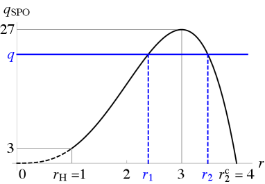
Outside the horizon, has a unique local maximum with the value at . Eliminating from Eqs. (21) and (22), we obtain the extremum values as
| (23) |
where () are the radii of SPOs and are the real solutions of . Note that () increases (decreases) monotonically with in the range
| (24) |
where is the radius of the unstable photon circular orbit. The number of real roots of outside the horizon depends on . There exists a single root for , while there exist two roots and for . For , coincide with each other at , so that coincide with . Figure 1 shows a relation between and the radii .
III Photon Escape Condition
We consider the escape condition of a photon emitted from an arbitrary spacetime position . Since the Kerr black hole spacetime is reflection symmetric with respect to the equatorial plane , we consider only the range in what follows. The cases of and will be considered in Appendix A.
The necessary and sufficient conditions for photons to escape are that they have appropriate parameters to reach infinity from (necessary condition) and are in the allowed region determined by the variable . In the following subsections, we consider the photon escape conditions for and separately.
III.1 Necessary condition for photon escape,
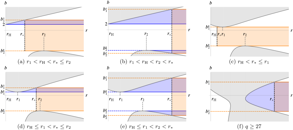
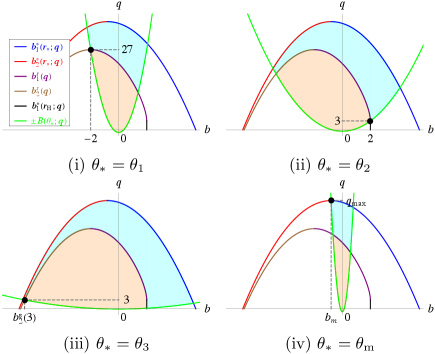
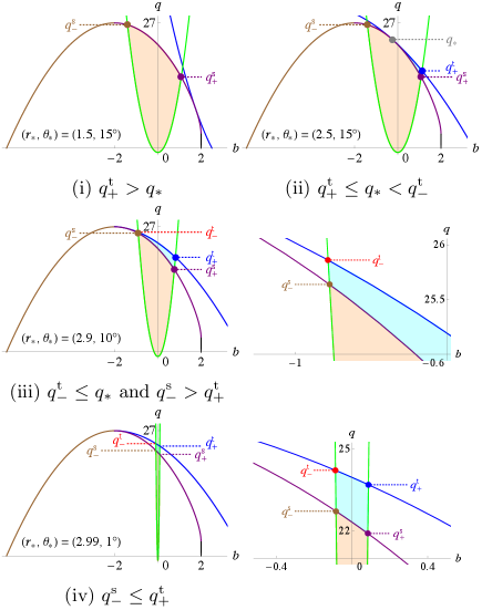
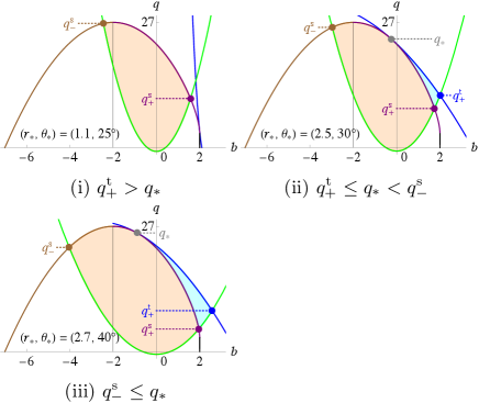
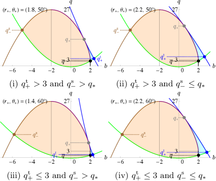
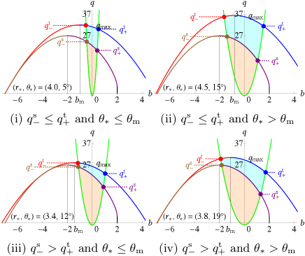
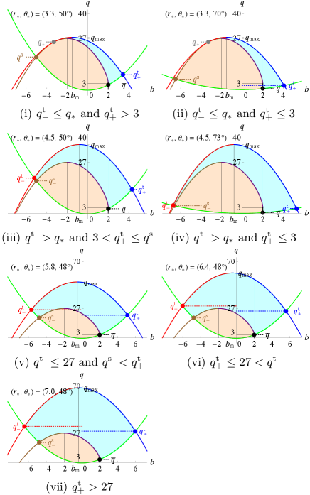
Let us consider the behavior of to determine the range of in which photons with satisfy the necessary condition to escape from to infinity. We can see the typical shape of as gray curves in Figs. 2(a) and 2(b) for , in Figs. 2(c)–2(e) for , and in Fig. 2(f) for . Gray regions denote forbidden regions of photon motion. Orange and blue regions represent the parameter range of where photons satisfy a necessary condition for escape with and , respectively.
In the case , photons initially emitted outward (i.e., ) with can escape [see orange region in Fig. 2(a)], and photons initially emitted inward (i.e., ) with also can escape [see blue region in Fig. 2(a)], where
| (25) |
In the case , photons initially emitted outward (i.e., ) with can escape [see orange region in Fig. 2(b)], and photons initially emitted inward (i.e., ) with or also can escape [see blue region in Fig. 2(b)].
In the case , only photons initially emitted outward (i.e., ) with can escape [see orange region in Fig. 2(c)].
In the case , photons initially emitted outward (i.e., ) with can escape [see orange region in Fig. 2(d)], and photons initially emitted inward (i.e., ) with also can escape [see blue region in Fig. 2(d)].
In the case , photons initially emitted outward (i.e., ) with can escape [see orange region in Fig. 2(e)], and photons initially emitted inward (i.e., ) with or also can escape [see blue region in Fig. 2(e)].
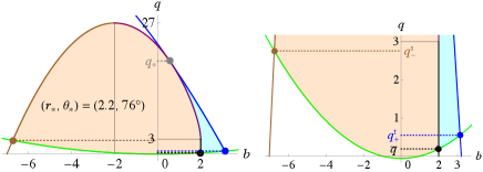
For , the allowed region is disconnected. Therefore, if is in the outer allowed region, photons must have and always can escape [see orange and blue region in Fig. 2(f)].
| Radial position of an emitter | () | () | Shape of | |
| (i) | Fig. 2(a) | |||
| Fig. 2(d) | ||||
| n/a | Fig. 2(c) | |||
| (ii) | Fig. 2(a) | |||
| Fig. 2(d) | ||||
| , | Fig. 2(e) | |||
| Fig. 2(f) | ||||
| (iii) | Fig. 2(a) | |||
| , | Fig. 2(b) | |||
| , | Fig. 2(e) | |||
| Fig. 2(f) | ||||
| (iv) | , | Fig. 2(b) | ||
| , | Fig. 2(e) | |||
| Fig. 2(f) |
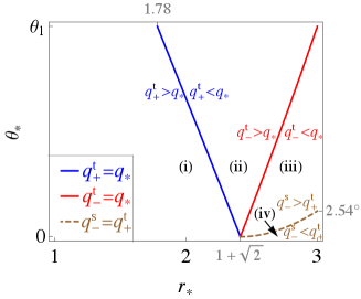
Let us summarize the necessary condition for photon escape in the () parameter region for a fixed . To perform it, we introduce four ranges of :
| (26) | ||||
| (27) | ||||
| (28) | ||||
| (29) |
where is the largest solution of . In addition, we introduce two specific values of ,
| (30) | ||||
| (31) |
When , the functions coincide with each other, and their value is
| (32) |
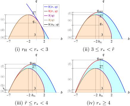
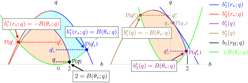
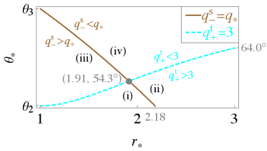
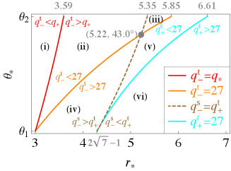
When , the position enters the forbidden region. Therefore, the maximum value of is limited by . The necessary conditions for photon escape are summarized in Table 1.111Note that in Refs. Ogasawara:2019mir ; Ogasawara:2020frt , the photon escape regions were considered only for the case (i), i.e., . Here, we identify them for the entire range of . It is useful to visualize the necessary condition for photon escape in the - plane; see Fig. 3. The blue, red, purple, and brown curves denote , , , and , respectively. The black segment denotes and . The orange regions show the parameter regions where photons initially emitted outward (i.e., ) satisfy the necessary condition for escape. The cyan regions show the parameter regions where photons initially emitted both outward and inward (i.e., ) satisfy the necessary condition for escape. Figures 3(i)–3(iv) correspond to Tables 1(i)–1(iv), respectively.
III.2 Necessary and sufficient condition for photon escape,
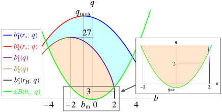
Let us further restrict the above necessary condition for photon escape by the non-negativity of , i.e., Eq. (19). The common region of these conditions provides the necessary and sufficient parameter region in which a photon can escape from to infinity. We call it the escapable region. An example of the escapable region is seen in Fig. 4. The green curve denotes , and the other curves and colored regions are the same as in Fig. 3. We can find that the escapable region corresponds to the regions in Fig. 3 further restricted by the condition (19).
III.3 Necessary and sufficient condition for photon escape,
We identify the escapable region for . The negative together with the non-negativity of at leads to
| (33) |
This implies that for , and the minimum value of is given at as
| (34) |
For , the SPOs are not relevant to photon escape because they do not exist. Therefore, we only focus on , or equivalently,
| (35) |
The right-hand side is positive for all and . Hence, the allowed region (35) contains the entire parameter region (33). This means that any radial turning point no longer appears for . Finally, we conclude that photons with can escape to infinity if they are initially emitted outward (i.e., ) and take the range (33). Figure 4 shows an example of the escapable region (see the orange region of ).
IV Critical values for classifying photon escape
In order to classify the escapable region completely, we introduce the critical polar angles and the critical values of .
IV.1 Critical angles
We introduce four critical polar angles , , , and , at which the classification of the escapable region varies qualitatively. Solving for , we obtain a solution
| (36) |
see Appendix B.
The first special point is , where and coincide with each other. We define as at which passes through , i.e., [see the black dot in Fig. 5(i)]. Then, is given by
| (37) |
When , holds in the range . This implies that the minimum value of in the escapable region for is always .
The second special point is , where and . We define as at which passes through , i.e., [see the black dot in Fig. 5(ii)]. Then, is given by
| (38) |
When , holds in the range . This implies that the maximum value of in the escapable region for is always .
The third special point is , where . We define as at which passes through , i.e., [see the black dot in Fig. 5(iii)]. Then, is given by
| (39) |
When , holds in the range . This implies that the minimum value of in the escapable region for is always .
The fourth special point is , where and coincide with each other. We define as at which passes through , i.e., [see the black dot in Fig. 5(iv)]. Then, is given by
| (40) |
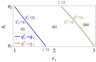
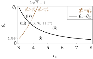
Note that we only need to consider for because it does not contribute to specifying the escapable region when . The critical angle depends on and monotonically decreases with in the range
| (41) |
When , holds in the range . This implies that the minimum value of in the escapable region for is always .
IV.2 Critical values of
We introduce five critical values , , and , as the values of at the intersections of , , , and , at which the classification of the parameter ranges varies qualitatively.
We define as the value of at the intersection of and in the range , and we denote the intersection as P (see the black dot in Fig. 6). Then, is given by222This is expressed as in Ref. Ogasawara:2020frt
| (42) |
which only appears for and monotonically decreases with in the range
| (43) |
When , holds. This implies that the maximum value of in the escapable region for is always .
We define as the value of at the intersection of and , and we denote the intersection as P (see the blue dot in Fig. 6). On the other hand, we define as the value of at the intersection of and for and and for , and we denote the intersection as P (see the red dot in Fig. 6). Then, are given by333These and are expressed as and , respectively, in Ref. Ogasawara:2020frt .
| (44) |
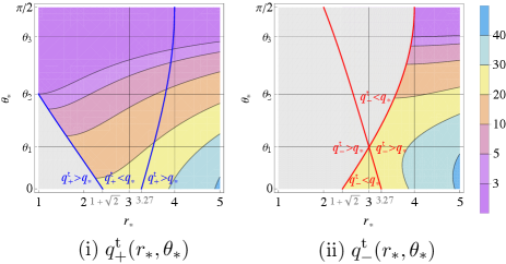
where only appears for . For , and coincide with each other at . Note that holds for all and . Figures 7(i) and 7(ii) show the values of and in the - parameter space, respectively.
We define as the value of at the intersection of and , and we denote the intersection as P (see the purple dot in Fig. 6). On the other hand, we define as the value of at the intersection of and for and and for , and we denote the intersection as P (see the brown dot in Fig. 6). Then, are given by444This is expressed as , and is expressed as for and as for , respectively, in Ref. Ogasawara:2020frt .
| (45) | ||||
| (46) |
where only appears for and monotonically decreases with in the range
| (47) |
As increases from to , begins with , monotonically increases to the maximum value at , and monotonically decreases to . For , and coincide with each other at .
In addition, we define as a point in the - plane that represents for and for (see the gray dot in Fig. 6).
These are summarized in Table 2.
| P | Intersection | ||
|---|---|---|---|
| and | |||
| and | |||
| and | |||
| and | |||
| and | |||
| – | for | ||
| for |
IV.3 Conditions for critical values of involved in classification
It is worth noting that and are not always involved in classification; i.e., the intersections P(), P(), and P are not always involved in classification.
When for , the intersection P() does not contribute to specifying the escapable region [see the gray region in Fig. 7(i)]. On the other hand, when for , the intersection P() is a special point, which contributes to specifying the escapable region. For , the intersection P() always contributes to it. The colored region in Fig. 7(i) represents the parameter region where contributes to specifying the escapable region.
For the same reason as for , the relative values of and determine whether contributes to specifying the escapable region. In the case of , only when for , the intersection P() is included in the escapable region. In the case of , when for and when , the intersection P is included. The colored region in Fig. 7(ii) represents the parameter region where contributes to specifying the escapable region.
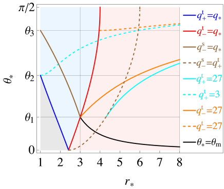
In the case of , when and when for , the point P() contributes to specifying the escapable region. In the case of , the point P() contributes to it only when for . The blue region in Fig. 8 represents the parameter region where contributes to specifying the escapable region.
Other intersections P() and P() contribute to specifying the escapable region when and , respectively, and P() always contributes to it.
In the following section, we will perform a complete classification of photon escape.
V Complete classification of photon escape in the extremal Kerr black hole
| Class | Range of | Characteristic ’s |
|---|---|---|
| I | and | , , and |
| II | and | , , and |
| III | and | , , , , and |
| IV | and | , , , , and |
| V | and | and |
| VI | and | , , , and |
| VII | and | , , , , , and |
| VIII | and | , , , , , and |
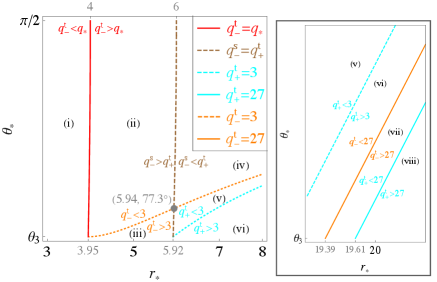
In this section, we make a complete classification of photon escape. We define eight classes according to a spacetime position of an emitter (see Table 3):
| (48) | ||||
| (49) | ||||
| (50) | ||||
| (51) | ||||
| (52) | ||||
| (53) | ||||
| (54) | ||||
| (55) |
For (i.e., classes I–IV), monotonically increases with in the range
| (56) |
and we only need to consider the range of because there is no escapable region in . For (i.e., classes V–VIII), as increases from to , begins at and monotonically decreases to . We only need to consider the range of because there is no escapable region in .
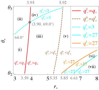
Figure 8 shows the relationship of the characteristic ’s in the - parameter space. In the gray region, and do not contribute to specifying the escapable region. In the blue region, and contribute to specifying the escapable region, while does not. In the red region, contribute to specifying the escapable region, while does not. For each class, the regions separated by these curves give different escapable parameter regions. For example, since the region and (i.e., class I) is divided into four by three curves, there are four different cases of the escapable regions. Note that the curve representing for is not plotted because it does not contribute to the classification of photon escape. Also, for the same reason, the curve representing for and , and for and is not plotted.
In the following subsections, we consider the escapable region separately for each class.
V.1 Class I: and
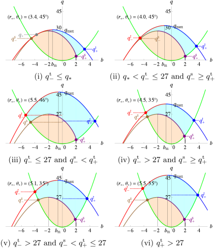
There exist four cases according to the relative values of , , and (see Fig. 9):
| (57) | ||||
| (58) | ||||
| (59) | ||||
| (60) |
where case (iv) appears only when . The equal signs of Eqs. (58) and (59) hold only when and , respectively. Note that contributes to specifying the escapable region only for case (ii), contributes to that for cases (ii)–(iv), and contributes to that for cases (iii) and (iv). The escapable regions in the above cases are summarized in Table 4 and Fig. 10.
| Case | () | () | |
|---|---|---|---|
| (i)–(iv) | n/a | ||
| (ii) and (iii) | |||
| (iv) | |||
| (ii) | |||
| (iii) | |||
| (i) | n/a | ||
| (ii) | |||
| (iv) | |||
| (iii) | |||
| (iv) | |||
| (i) and (ii) | n/a | n/a | |
| (iii) and (iv) | n/a | n/a |
V.2 Class II: and
There exist three cases according to the relative values of , , and (see Fig. 11):
| (61) | ||||
| (62) | ||||
| (63) |
where the equal sign of Eq. (62) holds only when . For case (i), and do not contribute to specifying the escapable region. The escapable regions in the above cases are summarized in Table 5 and Fig. 12.
V.3 Class III: and
V.4 Class IV: and
V.5 Class V: and
There are four cases according to the relative values of and , and and (see Fig. 16):
| Case | () | () | |
| (i)–(iii) | n/a | ||
| (ii) and (iii) | |||
| (ii) | |||
| (iii) | |||
| (i) | n/a | ||
| (ii) | |||
| (iii) | |||
| (i) and (ii) | n/a | ||
| (iii) |
| (68) | ||||
| (69) | ||||
| (70) | ||||
| (71) |
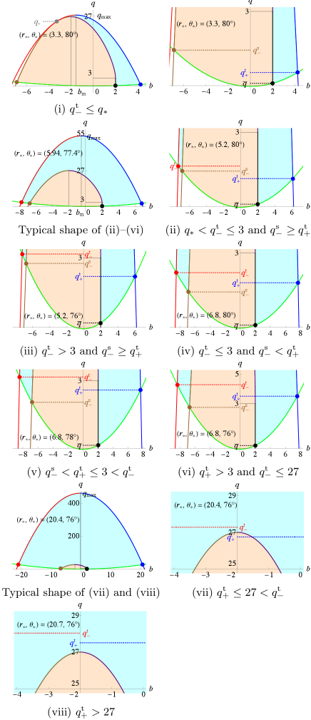
The escapable regions in the above cases are summarized in Table 8 and Fig. 17. Note that the shape of the escapable region of class V(i) is the same as that of class I(iv), and the shape of the escapable region of class V(iii) is the same as that of class I(iii).
| Case | () | () | |
| (i)–(iv) | n/a | ||
| (i) and (ii) | |||
| (iii) and (iv) | |||
| (i) | |||
| (ii) | |||
| (iii) | |||
| (iv) | |||
| (i) and (iii) | n/a | ||
| n/a | |||
| (ii) and (iv) | |||
| n/a |
| () | () | |
|---|---|---|
| n/a | ||
| n/a |
V.6 Class VI: and
There are six cases according to the relative values of , , , and (see Fig. 18):
| (72) | ||||
| (73) | ||||
| (74) | ||||
| (75) | ||||
| (76) | ||||
| (77) |
where contributes to specifying the escapable region only for case (i), and contributes to that for cases (ii)–(vi). The escapable regions in the above cases are summarized in Table 9 and Fig. 19.
| Case | () | () | |
|---|---|---|---|
| (i)–(iv) | n/a | ||
| (i) and (ii) | |||
| (iii) and (iv) | |||
| (i) and (ii) | |||
| (iii) and (iv) | |||
| (i) and (ii) | |||
| (iii) and (iv) | |||
| (i) and (iii) | n/a | n/a | |
| (ii) and (iv) |
| Case | () | () | |
|---|---|---|---|
| (i)–(vi) | n/a | ||
| (i), (ii), (iv) | |||
| (iii), (v), (vi) | |||
| (iii) and (v) | |||
| (vi) | and | ||
| (i) | |||
| (ii) | |||
| (iii) | and | ||
| (iv) | |||
| (v) | |||
| (vi) | |||
| (i) | |||
| (ii) and (iii) | and | ||
| (iv) and (v) | |||
| (vi) | |||
| (i)–(iii) | |||
| (iv)–(vi) |
V.7 Class VII: and
There are seven cases according to the relative values of , , , , and (see Fig. 20):
| (78) | ||||
| (79) | ||||
| (80) | ||||
| (81) | ||||
| (82) | ||||
| (83) | ||||
| (84) |
where contributes to specifying the escapable region for cases (i) and (ii), and contributes to that for cases (ii)–(vii). The escapable regions in the above cases are summarized in Table 10 and Fig. 21.
Note that solving and for , we obtain and , respectively.
| Case | () | () | |
|---|---|---|---|
| (i)–(vii) | n/a | ||
| (i), (iii), (v)–(vii) | |||
| (ii) and (iv) | |||
| (i) and (iii) | |||
| (v)–(vii) | |||
| (ii) and (iv) | |||
| (i) and (iii) | |||
| (ii) and (iv) | |||
| (i) and (ii) | |||
| (v) and (vi) | |||
| (vii) | and | ||
| (iii) and (iv) | |||
| (v) | and | ||
| (vi) | |||
| (i) and (ii) | |||
| (iii)–(v) | and | ||
| (vii) | |||
| (vi) | |||
| (vii) | |||
| (i)–(v) | |||
| (vi) and (vii) |
V.8 Class VIII: and
There are eight cases according to the relative values of , , , , and (see Fig. 22):
| (85) | ||||
| (86) | ||||
| (87) | ||||
| (88) | ||||
| (89) | ||||
| (90) | ||||
| (91) | ||||
| (92) |
where contributes to specifying the escapable region only for case (i), and contributes to that for cases (i)–(viii). The escapable regions in the above cases are summarized in Table 11 and Fig. 23.
| Case | () | () | |
|---|---|---|---|
| (i)–(viii) | n/a | ||
| (i)–(iii) | |||
| (iv) and (v) | |||
| (vi)–(viii) | |||
| (i)–(iii) | |||
| (iv) and (v) | |||
| (vi)–(viii) | and | ||
| (i) | |||
| (ii) | |||
| (iii) | and | ||
| (iv) | |||
| (v) | |||
| (ii) and (iv) | |||
| and | |||
| (vi) and (vii) | |||
| (viii) | and | ||
| (iii) and (v) | |||
| (vi) | and | ||
| (vii) | |||
| (i) | |||
| (ii) and (iv) | and | ||
| (iii), (v), (vi) | |||
| (viii) | |||
| (vii) | |||
| (viii) | |||
| (i)–(vi) | |||
| (vii) and (viii) |
VI DISCUSSION
We have completely classified the necessary and sufficient range of the impact parameters for photons emitted from an arbitrary spacetime position of the extremal Kerr black hole to escape to infinity, i.e., the escapable regions. The radial equation of motion determines the necessary conditions for photons emitted from to escape to infinity, and the polar angle equation of motion further restricts the allowed region of photon motion. In the process of classifying photon escape, we have defined four critical angles at which the classification of the escapable region varies qualitatively and five critical values of at which the classification of the impact parameter range varies qualitatively. We have divided the entire spacetime into eight regions by three critical angles and , class I–VIII. Furthermore, we have appropriately selected the critical values of contributing to specifying the escapable region and have completely classified the difference in the shape of the escapable region, that is, the difference in the escapable parameter range, according to the relative values of critical ’s. Our main results are summarized in the tables of Sec. V.
This study has generalized our previous result Ogasawara:2020frt , which focused only on light sources near the horizon, to the classification that covers light sources in the entire region. We have considered the extremal Kerr black hole here, but our classification method can be directly applied to nonextremal Kerr black holes. Furthermore, since this method also can be applied to timelike particles, it will be possible to discuss the neutrino radiation Wang:2021elf , the escape of high-energy particles in high-energy astrophysics, e.g., the collisional Penrose process Piran:1975apj ; Schnittman:2018ccg , and high-energy particle collision Banados:2009pr ; Harada:2014vka .
As we have mentioned in the Introduction, evaluating a photon escape probability is essential to reveal the observability of phenomena around a black hole. In the calculation of the escape probability, it is necessary to specify not only an emitter’s position but also its proper motion. However, since our complete set of the escapable regions is independent of the proper motion, the set provides a basis for evaluating the escape probability. Based on the classification in the present paper, we will report the escape cone and probability for various states of an emitter in a forthcoming paper Ogasawara:tbp .
Acknowledgements.
The authors are grateful to Takahiro Tanaka, Kouji Nakamura, Kazunori Kohri, and Takahiro Matsubara for useful comments. This work was supported by JSPS KAKENHI Grants No. JP20J00416 and No. JP20K14467 (K.O.) and Grant No. JP19K14715 (T.I.).Appendix A Photon escape for and
A.1
We consider photon escape in the case . When , the regularity of the function [Eq. (11)] requires . Substituting it into , we have .
We focus on the negative range . As shown in Sec. III.3, the non-negativity of the function gives the allowed parameter range of . Combining the inequality (35) with and , we have
| (93) |
Since this inequality always holds outside the horizon, all of the photons emitted outwardly with can escape to infinity.
Next, we focus on the non-negative range of . In this case, coincide with each other and also coincide with each other, and their values are given by
| (94) | ||||
| (95) |
Note that holds outside the horizon and the equal sign holds only when . There are two cases depending on the radial position of the emitter:
| (96) | ||||
| (97) |
The escapable regions in the above cases are summarized in Table 12.
| Case | () | () | |
| (i) | n/a | ||
| n/a | n/a | ||
| (ii) | n/a | ||
| n/a | |||
| n/a | n/a |
A.2
Appendix B Equation for the polar angle of Kerr geodesics
We focus on the function , which appears in the geodesic equation for the polar angle direction of the Kerr spacetime. We consider the following equation:
| (98) |
where , , are constants, and . For , the constant must vanish, and must hold. We assume in what follows. Equation (98) is rewritten as an equivalent equation in terms of ,
| (99) |
Solving Eq. (99) for , we obtain
| (100) |
In order for to be real, the parameters must satisfy the inequality
| (101) |
which also guarantees positive. On the other hand, the condition is written as
| (102) |
where the double sign corresponds to that in Eq. (100). For the upper case, the parameters must satisfy and . For the lower case, if together with Eq. (101), then the inequality (102) holds; if , then must hold.
Now we introduce new combinations of the parameters
| (103) |
which satisfy the following relations:
| (104) | ||||
| (105) | ||||
| (106) |
Using these, we can rewrite Eq. (100) in terms of as
| (107) |
Because of the range of , we can take the positive branch
| (108) |
Finally we obtain
| (112) |
References
- (1) K. Akiyama et al. (Event Horizon Telescope Collaboration), First M87 Event Horizon Telescope results. I. The shadow of the supermassive black hole, Astrophys. J. 875, L1 (2019).
- (2) V. Cardoso and P. Pani, Testing the nature of dark compact objects: A status report, Living Rev. Relativity 22, 4 (2019).
- (3) J. L. Synge, The escape of photons from gravitationally intense stars, Mon. Not. R. Astron. Soc. 131, 463 (1966).
- (4) K. Ogasawara, T. Igata, T. Harada, and U. Miyamoto, Escape probability of a photon emitted near the black hole horizon, Phys. Rev. D 101, 044023 (2020).
- (5) O. Semerak, Photon escape cones in the Kerr field, Helv. Phys. Acta 69, 69 (1996).
- (6) Z. Stuchlík, D. Charbulák, and J. Schee, Light escape cones in local reference frames of Kerr–de Sitter black hole spacetimes and related black hole shadows, Eur. Phys. J. C 78, 180 (2018).
- (7) M. Zhang and J. Jiang, Emissions of photons near the horizons of Kerr-Sen black holes, Phys. Rev. D 102, 124012 (2020).
- (8) R. Takahashi and M. Takahashi, Anisotropic radiation field and trapped photons around the Kerr black hole, Astron. Astrophys. 513, A77 (2010).
- (9) T. Igata, K. Nakashi, and K. Ogasawara, Observability of the innermost stable circular orbit in a near-extremal Kerr black hole, Phys. Rev. D 101, 044044 (2020).
- (10) D. E. A. Gates, S. Hadar, and A. Lupsasca, Maximum observable blueshift from circular equatorial Kerr orbiters, Phys. Rev. D 102, 104041 (2020).
- (11) D. E. A. Gates, S. Hadar, and A. Lupsasca, Photon emission from circular equatorial Kerr orbiters, Phys. Rev. D 103, 044050 (2021).
- (12) R. Abuter et al. (GRAVITY Collaboration 2020), Detection of the gravitational redshift in the orbit of the star S2 near the Galactic centre massive black hole, Astron. Astrophys. 615, L15 (2018).
- (13) H. Saida et al., A significant feature in the general relativistic time evolution of the redshift of photons coming from a star orbiting Sgr A*, Publ. Astron. Soc. Jpn. 71, 126 (2019).
- (14) Y. Iwata, T. Oka, M. Tsuboi, M. Miyoshi, and S. Takekawa, Time variations in the flux density of Sgr A* at 230 GHz detected with ALMA, Astrophys. J. Lett. 892, L30 (2020).
- (15) T. Igata, K. Kohri, and K. Ogasawara, Photon emission from inside the innermost stable circular orbit, Phys. Rev. D 103, 104028 (2021).
- (16) H. Yan, M. Guo, and B. Chen, Observability of zero-angular-momentum sources near Kerr black holes, Eur. Phys. J. C 81, 847 (2021).
- (17) H. Yan, Z. Hu, M. Guo, and B. Chen, Photon emissions from NHEK and near-NHEK equatorial emitters, Phys. Rev. D 104, 124005 (2021).
- (18) K. Ogasawara and T. Igata, Complete classification of photon escape in the Kerr black hole spacetime, Phys. Rev. D 103, 044029 (2021).
- (19) M. Walker and R. Penrose, On quadratic first integrals of the geodesic equations for type {22} spacetimes, Commun. Math. Phys. 18, 265 (1970).
- (20) B. Carter, Global structure of the Kerr family of gravitational fields, Phys. Rev. 174, 1559 (1968).
- (21) E. Teo, Spherical photon orbits around a Kerr black hole, Gen. Relativ. Gravit. 35, 1909 (2003).
- (22) J. S. Wang, J. Tseng, S. Gullin, and E. P. O’Connor, Non-radial neutrino emission upon black hole formation in core collapse supernovae, arXiv:2109.11430 [astro-ph]. Phys. Rev. D 104, 104030 (2021).
- (23) T. Piran, J. Shaham, and J. Katz, High efficiency of the Penrose mechanism for particle collisions, Astrophys. J. 196, L107 (1975).
- (24) J. D. Schnittman, The collisional Penrose process, Gen. Relativ. Gravit. 50, 77 (2018).
- (25) M. Banados, J. Silk, and S. M. West, Kerr Black Holes as Particle Accelerators to Arbitrarily High Energy, Phys. Rev. Lett. 103, 111102 (2009).
- (26) T. Harada and M. Kimura, Black holes as particle accelerators: A brief review, Classical Quantum Gravity 31, 243001 (2014).
- (27) K. Ogasawara and T. Igata (to be published).