Photon spheres, ISCOs, and OSCOs: Astrophysical observables for regular black holes with asymptotically Minkowski cores

Thomas Berry , Alex Simpson , and Matt Visser

Abstract

Classical black holes contain a singularity at their core. This has prompted various researchers to propose a multitude of modified spacetimes that mimic the physically observable characteristics of classical black holes as best as possible, but that crucially do not contain singularities at their cores. Due to recent advances in near-horizon astronomy, the ability to observationally distinguish between a classical black hole and a potential black hole mimicker is becoming increasingly feasible. Herein, we calculate some physically observable quantities for a recently proposed regular black hole with an asymptotically Minkowski core — the radius of the photon sphere and the extremal stable timelike circular orbit (ESCO). The manner in which the photon sphere and ESCO relate to the presence (or absence) of horizons is much more complex than for the Schwarzschild black hole. We find situations in which photon spheres can approach arbitrarily close to (near extremal) horizons, situations in which some photon spheres become stable, and situations in which the locations of both photon spheres and ESCOs become multi-valued, with both ISCOs (innermost stable circular orbits) and OSCOs (outermost stable circular orbits). This provides an extremely rich phenomenology of potential astrophysical interest.

Date:
Monday 31 August 2020; Monday 7 September; LaTeX-ed

Keywords: regular black hole, Minkowski core, Lambert $W$ function, black hole mimic.

PhySH: Gravitation

1 Introduction

Karl Schwarzschild first derived the spacetime metric for the region exterior to a static, spherically symmetric source in 1916 [1]; only some 50 years later was it properly understood that this spacetime could be extrapolated inwards to describe a black hole. Without any loss of generality, any static spherically symmetric spacetime can be described by a metric of the form

\differential{s}^{2}=-\mathrm{e}^{-2\Phi(r)}\left(1-\frac{2m(r)}{r}\right)\differential{t^{2}}+\frac{\differential{r^{2}}}{1-\frac{2m(r)}{r}}+r^{2}\left(\differential{\theta^{2}}+\sin^{2}\theta\differential{\phi^{2}}\right).

(1.1)

For the standard Schwarzschild metric one sets $\Phi(r)=0$ and $m(r)=m_{0}$ . Over the past century, a vast host of black hole spacetimes, qualitatively distinct from that of Schwarzschild, have been investigated by multiple researchers [2, 3, 4, 5, 6, 7, 8, 9, 10, 11, 12, 13, 14].

Furthermore, the field has now grown to not only include classical black holes, but also quantum-modified black holes [15, 16, 17, 18], regular black holes [19, 20, 21, 22, 23], and various other exotic spherically symmetric spacetimes that are fundamentally different from black holes but mimic many of their observable phenomena (e.g. traversable wormholes [24, 25, 26, 27, 28, 31, 29, 30, 32, 33, 34, 35, 36, 37, 38, 39], gravastars [40, 41, 42, 43, 44, 45, 46], ultracompact objects [47, 48], etcetera [49, 50, 51]; see [52] for an in-depth discussion). Herein, we investigate a specific model spacetime representing a regular black hole. That is, a spacetime that has a well-defined horizon structure, but the curvature invariants are everywhere finite.

Investigating black hole mimickers is becoming increasingly relevant due to recent advances in both observational and gravitational wave astronomy. Projects such as the Event Horizon Telescope [53, 54, 55, 56, 57, 58], and LIGO [59, 60], and the planned LISA [61], are and will be continuously probing closer to the horizons of compact massive objects (CMOs), and so there is hope that such projects will eventually be able to distinguish between the near-horizon physics of classical black holes and possible astrophysical mimickers [52].

The model spacetime investigated in this work is a regular black hole with an asymptotically Minkowski core, as discussed in [62, 63]. This is an example of a metric with an exponential mass suppression, and is described by the line element

\differential s^{2}=-\left(1-\frac{2m\,\mathrm{e}^{-a/r}}{r}\right)\differential{t}^{2}+\frac{\differential{r}^{2}}{1-\frac{2m\,\mathrm{e}^{-a/r}}{r}}+r^{2}\left(\differential{\theta}^{2}+\sin^{2}\theta\differential{\phi}^{2}\right).

(1.2)

A rather different (extremal) version of this model spacetime, based on nonlinear electrodynamics, has been previously discussed by Culetu [64], with follow-up on some aspects of the non-extremal case in references [65, 66, 67]. See also [68, 69].

Most regular black holes have a core that is asymptotically de Sitter (with constant positive curvature) [19, 20, 21, 22]. However, the regular black hole described by the metric (1.2) has an asymptotically Minkowski core (in the sense that the stress-energy tensor asymptotes to zero). Such models have some attractive features compared to the more common de Sitter core regular black holes: the stress-energy tensor vanishes at the core, greatly simplifying the physics in this region; and many messy algebraic expressions are replaced by simpler expressions involving the exponential and Lambert $W$ functions, whilst still allowing for explicit closed form expressions for quantities of physical interest [62]. Additionally, the results obtained in this work reproduce the standard results for the Schwarzschild metric by letting the parameter $a\rightarrow 0$ . Thus, the value of the parameter $a$ determines the extent of the “deviation” from the Schwarzschild spacetime.

If $0<a<2m/\mathrm{e}$ then the spacetime described by the metric (1.2) has two horizons located at

r_{H^{-}}=2m\;\mathrm{e}^{W_{-1}\left(-\frac{a}{2m}\right)},\qquad\hbox{and}\qquad r_{H^{+}}=2m\;\mathrm{e}^{W_{0}\left(-\frac{a}{2m}\right)}.

(1.3)

Here $W_{-1}(x)$ and $W_{0}(x)$ are the real-valued branches of Lambert $W$ function. We could also write

r_{H^{-}}={a\over|W_{-1}\left(-\frac{a}{2m}\right)|},\qquad\hbox{and}\qquad r_{H^{+}}={a\over|W_{0}\left(-\frac{a}{2m}\right)|}.

(1.4)

Perturbatively, for small $a$ we have

r_{H^{+}}=2m-a+{\mathcal{O}}(a^{2}),

(1.5)

nicely reproducing Schwarzschild in the $a\to 0$ limit. For the inner horizon, since $r_{H_{-}}<2m$ then

r_{H^{-}}={a\over\ln(2m/r_{H_{-}})}

(1.6)

implies $r_{H^{-}}<a$ , whence we have a strict upper bound given by the simple analytic expression:

r_{H^{-}}<{a\over\ln(2m/a)}.

(1.7)

Certainly $\lim_{a\to 0}r_{H^{-}}(m,a)=0$ as we would expect to recover Schwarzschild; but the form of $r_{H^{-}}(m,a)$ is not analytic. This bound can also be viewed as the first term in an asymptotic expansion [70] based on (as $x\to 0^{+}$ )

W_{-1}(-x)=\ln(x)+{\mathcal{O}}(\ln(-\ln(x)))=-\ln(1/x)+{\mathcal{O}}(\ln(\ln(1/x))).

(1.8)

This leads to

r_{H^{-}}={a\over\ln(2m/a)+{\mathcal{O}}(\ln(\ln(2m/a)))}={a\over\ln(2m/a)}+{\mathcal{O}}\left(a\ln(\ln(2m/a))\over(\ln(2m/a))^{2}\right).

(1.9)

More specifically (as $a/m\to 0$ or $m/a\to\infty$ )

{r_{H^{-}}\over a}={1\over\ln(2m/a)}+{\mathcal{O}}\left(\ln(\ln(2m/a))\over(\ln(2m/a))^{2}\right).

(1.10)

If $a=2m/\mathrm{e}$ then the two horizons merge at $r_{H}=2m/\mathrm{e}=a$ and one has an extremal black hole. If $a>2m/\mathrm{e}$ then there are no horizons, and one is dealing with a regular horizonless extended but compact object, (the energy density peaks at $r=a/4$ ).

This object could either be extended all the way down to $r=0$ , or alternatively be truncated at some finite value of $r$ , to be used as the exterior geometry for some static and spherically symmetric mass source that isn’t a black hole. This is potentially useful as a model for planets, stars, etc. Consequently, we will also incorporate aspects of the analysis for $a>2m/\mathrm{e}$ as and when required to generate astrophysical observables in the case when equation (1.2) is modelling a compact object other than a black hole.

2 Geodesics and the effective potential

Continuing the analysis of [62], we will now calculate the location of the photon sphere and extremal stable circular orbit (ESCO) for the regular black hole with line element given by equation (1.2). Photon spheres, (or more precisely the closely related black hole silhouettes), have been recently observed for the massive objects M87 and Sgr A* [53, 54, 55, 56, 57, 58]. As such they are, along with the closely related ESCOs, practical and useful quantities to calculate for black hole mimickers.

We begin by considering the affinely parameterised tangent vector to the worldline of a massive or massless particle in our spacetime (1.2):

g_{\mu\nu}\derivative{x^{\mu}}{\lambda}\derivative{x^{\nu}}{\lambda}=-\left(1-\frac{2m\,\mathrm{e}^{-a/r}}{r}\right)\left(\derivative{t}{\lambda}\right)^{2}+\left(\frac{1}{1-\frac{2m\,\mathrm{e}^{-a/r}}{r}}\right)\left(\derivative{r}{\lambda}\right)^{2}\\ +r^{2}\left[\left(\derivative{\theta}{\lambda}\right)^{2}+\sin^{2}\theta\left(\derivative{\phi}{\lambda}\right)^{2}\right]=\epsilon,

(2.1)

where $\epsilon\in\{-1,0\}$ ; with $-1$ corresponding to a massive (timelike) particle and 0 corresponding to a massless (null) particle. (The case $\epsilon=+1$ would correspond to tachyonic particles following spacelike geodesics, a situation of no known physical applicability.) Since we are working with a spherically symmetric spacetime, we can set $\theta=\pi/2$ without any loss of generality and reduce equation (2.1) to

g_{\mu\nu}\derivative{x^{\mu}}{\lambda}\derivative{x^{\nu}}{\lambda}=-\left(1-\frac{2m\,\mathrm{e}^{-a/r}}{r}\right)\left(\derivative{t}{\lambda}\right)^{2}+\left(\frac{1}{1-\frac{2m\,\mathrm{e}^{-a/r}}{r}}\right)\left(\derivative{r}{\lambda}\right)^{2}+r^{2}\left(\derivative{\phi}{\lambda}\right)^{2}=\epsilon.

(2.2)

Due to the presence of time-translation and angular Killing vectors, we can now define the conserved quantities

E=\left(1-\frac{2m\,\mathrm{e}^{-a/r}}{r}\right)\left(\derivative{t}{\lambda}\right)\mbox{\quad and\quad}L=r^{2}\left(\derivative{\phi}{\lambda}\right),

(2.3)

corresponding to the energy and angular momentum of the particle, respectively. Thus, equation (2.2) implies

E^{2}=\left(\derivative{r}{\lambda}\right)^{2}+\left(1-\frac{2m\,\mathrm{e}^{-a/r}}{r}\right)\left(\frac{L^{2}}{r^{2}}-\epsilon\right).

(2.4)

This defines an “effective potential” for geodesic orbits

V_{\epsilon}(r)=\left(1-\frac{2m\,\mathrm{e}^{-a/r}}{r}\right)\left(\frac{L^{2}}{r^{2}}-\epsilon\right),

(2.5)

with the circular orbits corresponding to extrema of this potential.

3 Photon spheres

We subdivide the discussion into two topics: First the existence of circular photon orbits (photon spheres) and then the stability of circular photon orbits. The discussion is considerably more complex than for the Schwarzschild spacetime, where there is only one circular photon orbit, at $r=3m$ , and that circular photon orbit is unstable. Once the extra parameter $a$ is nonzero, and in particular sufficiently large, the set of photon orbits exhibits more diversity.

3.1 Existence of photon spheres

For null trajectories we have

V_{0}(r)=\left(1-\frac{2m\,\mathrm{e}^{-a/r}}{r}\right)\frac{L^{2}}{r^{2}}.

(3.1)

So for circular photon orbits

V_{0}^{\prime}(r_{c})=\frac{2L^{2}}{r_{c}^{5}}\left[m\,\mathrm{e}^{-a/r_{c}}(3r_{c}-a)-r_{c}^{2}\right]=0.

(3.2)

To be explicit about this, the location of a circular photon orbit, $r_{c}$ , is given implicitly by the equation

r_{c}^{2}=m\,\mathrm{e}^{-a/r_{c}}(3r_{c}-a),

(3.3)

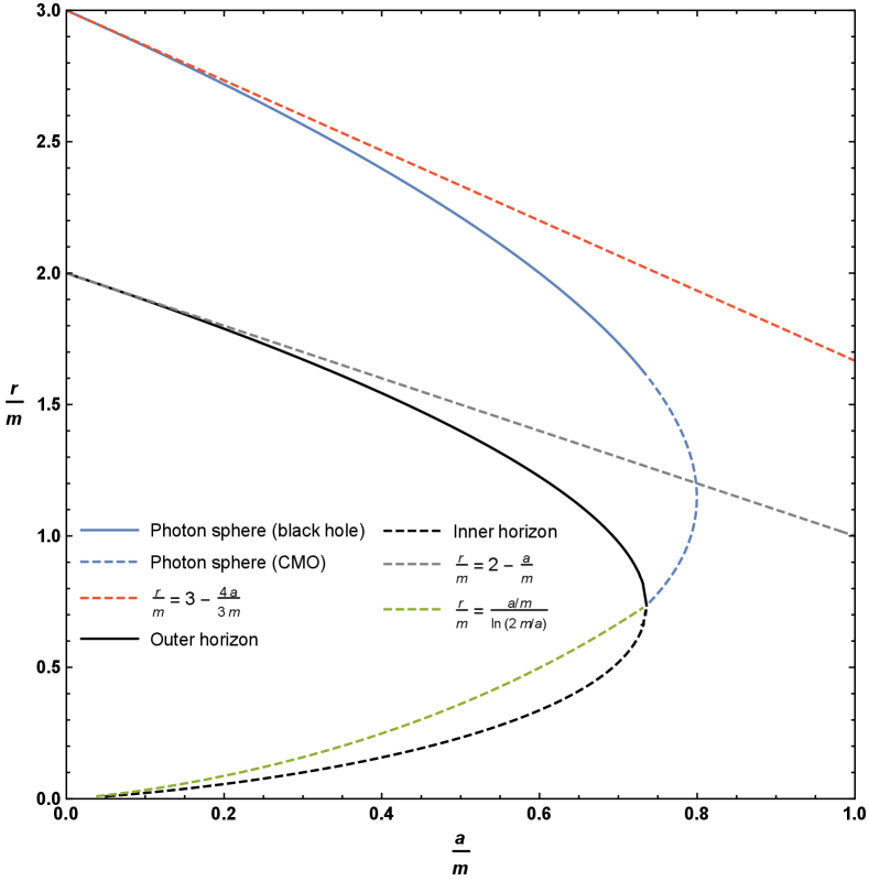
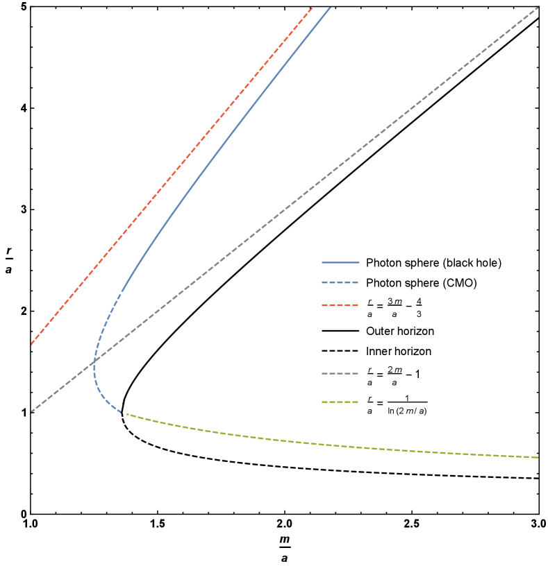
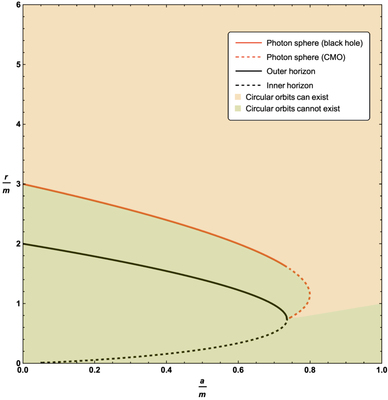
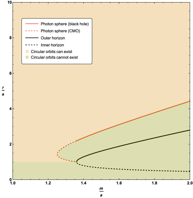
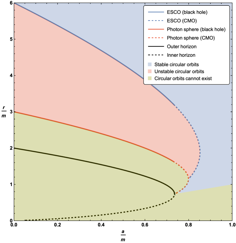
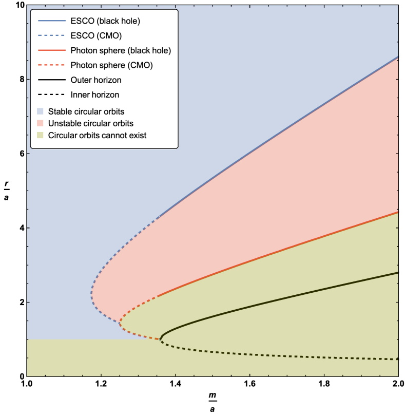
where $a$ and $m$ are fixed by the geometry of the spacetime.¹¹1As $a\to 0$ we have $r_{c}\to 3m$ , as expected for Schwarzschild spacetime. The curve described by the loci of these circular photon orbits has been plotted in two distinct ways in Figure 1.

For clarity, defining $w=r_{c}/a$ and $z=m/a$ , we can re-write the condition for circular photon orbits as

w^{2}=z\,\mathrm{e}^{-1/w}(3w-1);\qquad\implies\qquad z={w^{2}\;\mathrm{e}^{1/w}\over 3w-1}.

(3.4)

In Figure 1 we also plot the locations of both inner and outer horizons.

The inner and outer horizons merge at $a/m=2/\mathrm{e}=0.7357588824...$ ; that is, at $m/a=\mathrm{e}/2=1.359140914...$ . For $a/m>2/\mathrm{e}$ ; that is for $m/a<\mathrm{e}/2$ ; one is dealing with a horizonless compact object and we see that there is a region where there are two circular photon orbits. Note that the curve described by the loci of circular photon orbits terminates once one hits a horizon, that is, at $w=1$ . Sub-horizon curves of constant $r$ are spacelike (tachyonic), and cannot be lightlike, so they are explicitly excluded. That is, photon spheres can only exist in the region $w\in(1,\infty)$ .

Can we be more explicit about the key qualitative and quantitative features of this plot? Specifically, let us now analyze stability versus instability, and find the exact location of the various turning points.

3.2 Stability versus instability for circular photon orbits

To check the stability of these circular photon orbits we now need to investigate

V_{0}^{\prime\prime}(r_{c})=\frac{2L^{2}}{r_{c}^{7}}\left[3r_{c}^{3}-m\,\mathrm{e}^{-a/r_{c}}(6r_{c}-a)(2r_{c}-a)\right].

(3.5)

3.2.1 Perturbative analysis (small $a$ )

We note that determining $r_{c}(m,a)$ from equation (3.3) is not analytically feasible, but $r_{c}(m,a)$ can certainly be estimated perturbatively for small $a$ . We have

r_{c}(m,a)=3m-\frac{4ma}{r_{c}}+\mathcal{O}(a^{2})\quad\implies\quad r_{c}(m,a)=3m-{4\over 3}a+\mathcal{O}(a^{2}).

(3.6)

So, for small values of $a$ , we recover the standard result for the location of the photon sphere in Schwarzschild spacetime.

Estimating $V_{0}^{\prime\prime}(r_{c})$ by now substituting the approximate location of the photon sphere as $r_{c}(m,a)=3m-4a/3+\mathcal{O}(a^{2}),$ we find

V_{0}^{\prime\prime}(r_{c}(m,a))=-{2L^{2}\over 81m^{4}}\left(1+{4\over 3}\,{a\over m}+\mathcal{O}(a^{2})\right).

(3.7)

This quantity is manifestly negative for small $a$ . That is, (within the limits of the current small- $a$ approximation), photons are in an unstable orbit at the small- $a$ photon sphere.

3.2.2 Non-perturbative analysis

However, if we rephrase the problem then we can make some much more explicit exact statements that are no longer perturbative in small $a$ : Whereas determining $r_{c}(m,a)$ is analytically infeasible it should be noted that in contrast both $a(m,r_{c})$ and $m(r_{c},a)$ are easily determined analytically:

a(m,r_{c})=r_{c}(3-W(r_{c}\mathrm{e}^{3}/m));\qquad m(r_{c},a)={r_{c}^{2}\;\mathrm{e}^{a/r_{c}}\over(3r_{c}-a)}.

(3.8)

Consequently, at the peak we can write

V_{0}(r_{c},m)={L^{2}\over r_{c}^{2}}\left(1-{2\over W(r_{c}\mathrm{e}^{3}/m)}\right);\qquad V_{0}(r_{c},a)={L^{2}\over r_{c}^{2}}\;{r_{c}-a\over 3r_{c}-a}.

(3.9)

Regarding stability, in the first case, substituting (3.8 a) into (3.5), we have

V_{0}^{\prime\prime}(r_{c},m)=-{2L^{2}\left(W(r_{c}\mathrm{e}^{3}/m)^{2}-W(r_{c}\mathrm{e}^{3}/m)-3\right)\over r_{c}^{4}W(r_{c}\mathrm{e}^{3}/m)}.

(3.10)

Using properties of the Lambert $W$ function, we quickly see that this is negative for $r_{c}/m>{1\over 2}(1+\sqrt{13})\;\mathrm{e}^{-5/2+\sqrt{13}/2}=1.146702958...$ , implying instability of the circular photon orbits in this region, (and stability outside this region).

That is, on the curve of circular photon orbits, $V^{\prime\prime}(r_{c})=0$ at the point

(r_{c}/m,a/m)_{*}=(1.146702958...,0.7995092385...).

(3.11)

In the second case, substituting (3.8 b) into (3.5), we have

V_{0}^{\prime\prime}(r_{c},a)=-{2L^{2}\over r_{c}^{5}}\;{3r_{c}^{2}-5ar_{c}+a^{2}\over 3r_{c}-a}.

(3.12)

This will certainly be negative for $r_{c}/a>(5+\sqrt{13})/6=1.434258546...$ , implying instability of the circular photon orbits in this region, (and stability outside this region).

That is, on the curve of circular photon orbits, $V^{\prime\prime}(r_{c})=0$ at the point

(r_{c}/a,m/a)_{*}=(1.434258546...,1.250767286...).

(3.13)

Consequently, on the curve of circular photon orbits we have existence and stability in the region $w\in(1,1.434258546...)$ ; and existence and instability in the region $w\in(1.434258546...,\infty)$ . Precisely at the point $w=1.434258546...$ the photon sphere exhibits neutral stability.

3.3 Turning points

To evaluate the exact location of the turning points on the curve described by the loci of circular photon orbits, recall that using $w=r_{c}/a$ and $z=m/a$ we can write this curve as

w^{2}=z\,\mathrm{e}^{-1/w}(3w-1)\qquad\implies\qquad z={w^{2}\mathrm{e}^{1/w}\over(3w-1)}.

(3.14)

This allows us to calculate

\derivative{z}{w}=\mathrm{e}^{1/w}\,\frac{3w^{2}-5w+1}{(3w-1)^{2}},

(3.15)

which has a zero located at $w=(5+\sqrt{13})/6$ , where we have already seen that $V_{0}^{\prime\prime}(r_{c},a)=V_{0}^{\prime\prime}(w)=0$ .

At this point $z$ takes on its maximum value

z=\mathrm{e}^{6/(5+\sqrt{13})}\frac{(5+\sqrt{13})^{2}}{18(3+\sqrt{13})}=\mathrm{e}^{(5-\sqrt{13})/2}\;{(2+\sqrt{13})\over 9}.

(3.16)

Consequently, no photon sphere can exist if

\frac{a}{m}>\mathrm{e}^{-(5-\sqrt{13})/2}\;(\sqrt{13}-2)=0.7995092385...;

(3.17)

or equivalently

\frac{m}{a}<\mathrm{e}^{(5-\sqrt{13})/2}\;{(2+\sqrt{13})\over 9}=1.250767286....

(3.18)

Note that this happens when

{r_{c}\over m}>{1\over 2}(1+\sqrt{13})\mathrm{e}^{-(5-\sqrt{13})/2};\qquad\qquad{r_{c}\over a}>{5+\sqrt{13}\over 6},

(3.19)

which was where, as we have already seen, $V_{0}^{\prime\prime}(r_{c},m)=0$ .

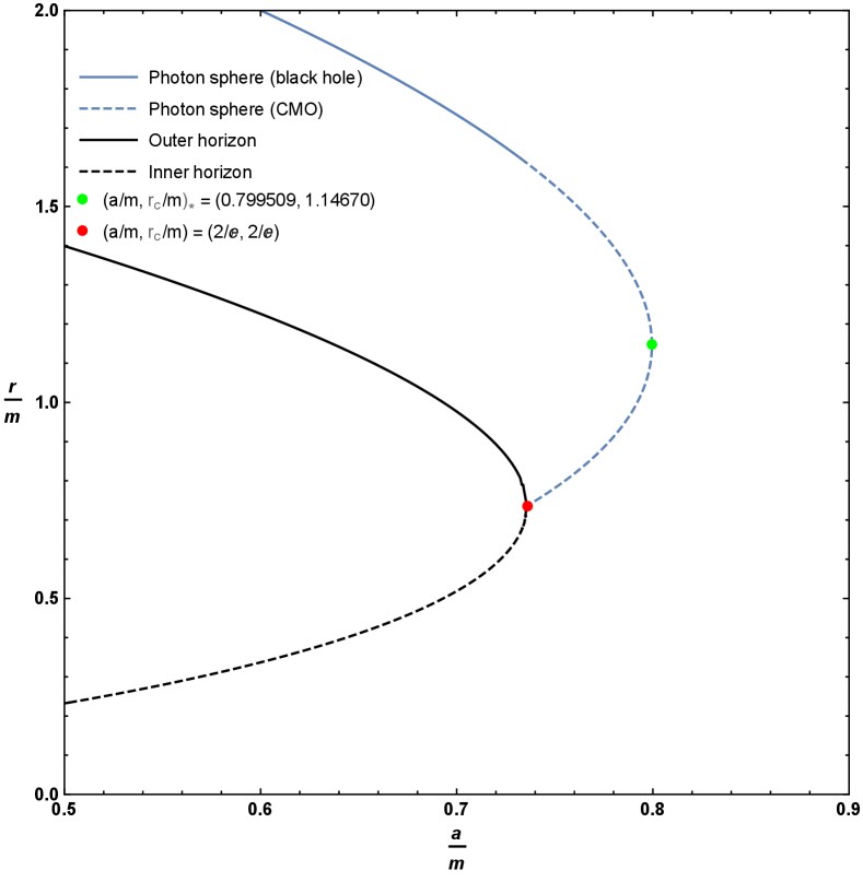
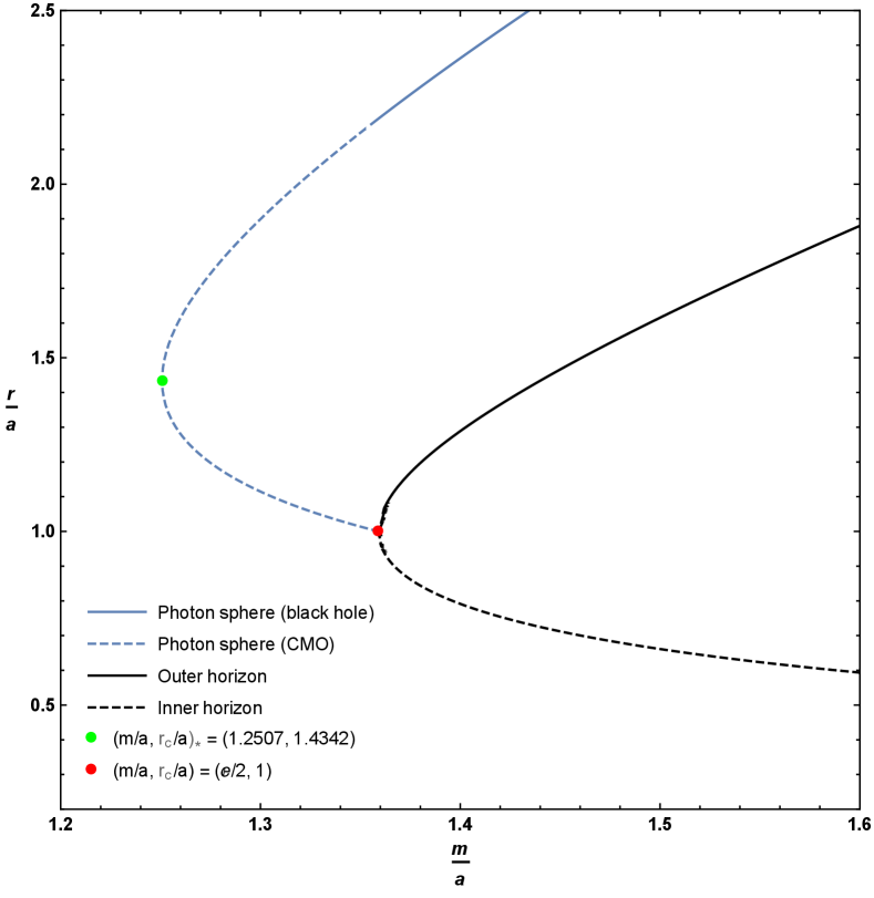
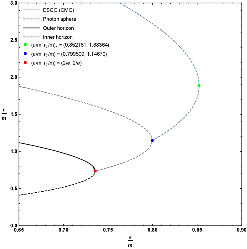
As can be seen, originally from Figure 1, and now in more detail in the zoomed-in plot in Figure 2, for horizonless compact massive objects there is a region where there are two possible locations for the photon sphere for fixed values of $m$ and $a$ . Furthermore when this happens it is the upper branch that corresponds to an unstable photon orbit, while the lower branch is a stable photon orbit.

4 Timelike circular orbits

Let us first check the existence, and then the stability, of timelike circular orbits. Even in Schwarzschild spacetime ( $a\to 0$ ) this is not entirely trivial: Timelike circular orbits exist for all $r_{c}\in(3m,\infty)$ ; they are unstable for $r_{c}\in(3m,6m)$ , exhibit neutral stability at $r_{c}=6m$ , and are stable for $r_{c}\in(6m,\infty)$ . Once the parameter $a$ is non-zero the situation is much more complex.

4.1 Existence of circular timelike orbits

For timelike trajectories, the effective potential is given by

V_{-1}(r)=\left(1-\frac{2m\,\mathrm{e}^{-a/r}}{r}\right)\left(1+\frac{L^{2}}{r^{2}}\right),

(4.1)

and so the locations of the circular orbits can be found from

V_{-1}^{\prime}(r_{c})=-\frac{2}{r_{c}^{5}}\left\{L^{2}r_{c}^{2}+m\,\mathrm{e}^{-a/r_{c}}[a(L^{2}+r_{c}^{2})-r_{c}(3L^{2}+r_{c}^{2})]\right\}=0.

(4.2)

That is, all timelike circular orbits (there will be infinitely many of them) must satisfy

L^{2}r_{c}^{2}+m\,\mathrm{e}^{-a/r_{c}}[a(L^{2}+r_{c}^{2})-r_{c}(3L^{2}+r_{c}^{2})]=0.

(4.3)

This is not analytically solvable for $r_{c}(L,m,a)$ , however we can solve for the required angular momentum $L_{c}(r_{c},m,a)$ of these circular orbits:

L_{c}(r_{c},m,a)^{2}={\frac{r_{c}^{2}\,m(r_{c}-a)}{ma-3mr_{c}+r_{c}^{2}\,\mathrm{e}^{a/r_{c}}}}.

(4.4)

Physically we must demand $0\leq L_{c}^{2}<\infty$ , so the boundaries for the existence region of circular orbits (whether stable or unstable) are given by

r_{c}=a;\qquad\qquad{ma-3mr_{c}+r_{c}^{2}\,\mathrm{e}^{a/r_{c}}}=0.

(4.5)

The first of these conditions $r_{c}=a$ , comes from the fact that in this spacetime gravity is effectively repulsive for $r<a$ . Remember that $g_{tt}=-(1-2m\mathrm{e}^{-a/r}/r)$ , and that the pseudo-force due to gravity depends on $\partial_{r}g_{tt}$ . Specifically

\partial_{r}g_{tt}=-{2m\over r^{2}}\;\mathrm{e}^{-a/r}\;\left(1-{a\over r}\right),

(4.6)

and this changes sign at $r=a$ . So for $r>a$ gravity attracts you to the centre, but for $r<a$ gravity repels you from the centre.

And if gravity repels you, there is no way to counter-balance it with a centrifugal pseudo-force, and so there is simply no way to get a circular orbit, regardless of whether it be stable or unstable. Precisely at $r=a$ there are stable “orbits” where the test particle just sits there, with zero angular momentum, no sideways motion required. Since by construction $r_{c}>r_{H^{+}}\geq a$ , this constraint is relevant only for horizonless CMOs.

The second of these conditions is exactly the location of the photon orbits considered in the previous sub-section. (Physically what is going on is this: At large distances it is easy to put a massive particle into a circular orbit with $L_{c}\propto\sqrt{mr_{c}}$ . As one moves inwards and approaches the photon orbit, the massive particle must move more and more rapidly, and the angular momentum per unit mass must diverge when a particle with nonzero invariant mass tries to orbit at the photon orbit.)

Thus the existence region (rather than just its boundary) for timelike circular orbits is therefore:

r_{c}>a;\qquad\qquad{ma-3mr_{c}+r_{c}^{2}\,\mathrm{e}^{a/r_{c}}}>0.

(4.7)

See Figure 3.

4.2 Stability versus instability for circular timelike orbits

Now consider the general expression

V_{-1}^{\prime\prime}(r)={6L^{2}r^{3}-2m(2r^{4}-4ar^{3}+(12L^{2}+a^{2})r^{2}-8L^{2}ar+L^{2}a^{2})\mathrm{e}^{-a/r}\over r^{7}},

(4.8)

and substitute the known value of $L\to L_{c}(r_{c})$ for circular orbits, see (4.4). Then

V_{-1}^{\prime\prime}(r_{c})=-{2me^{-a/r_{c}}(2m(3r_{c}^{2}-3ar_{c}+a^{2})\mathrm{e}^{-a/r_{c}}-r_{c}(r_{c}^{2}+ar_{c}-a^{2}))\over(r_{c}^{2}-m(3r_{c}-a)\mathrm{e}^{-a/r_{c}})r^{4}}.

(4.9)

Note that $V_{-1}^{\prime\prime}(r_{c})\to\infty$ at the photon orbit, (where the denominator has a zero).

To locate the boundary of the region of stable circular orbits, the ESCO (extremal stable circular orbit), we now need to set $V_{-1}^{\prime\prime}(r_{c})=0$ , leading to the equation

2m(3r_{c}^{2}-3ar_{c}+a^{2})\mathrm{e}^{-a/r_{c}}=r_{c}(r_{c}^{2}+ar_{c}-a^{2}).

(4.10)

We note that locating this boundary is equivalent to extremizing $L_{c}(r_{c})$ . To see this, consider the quantity $[V_{-1}^{\prime}(L(r),r)]=0$ and differentiate:

{\differential{}[V_{-1}^{\prime}(L(r),r)]\over\differential r}=\left.{\partial V_{-1}^{\prime}(L,r)\over\partial L}\right|_{L=L(r)}\times{\differential L(r)\over\differential r}+\left.V^{\prime\prime}_{-1}(L,r)\right|_{L=L(r)}.

(4.11)

This implies

0=\left.{\partial V_{-1}^{\prime}(L,r)\over\partial L}\right|_{L=L(r)}\times{\differential L(r)\over\differential r}\;+\;\left.V_{-1}^{\prime\prime}(L,r)\right|_{L=L(r)}.

(4.12)

Thence

\left.V_{-1}^{\prime\prime}(L,r)\right|_{L=L(r)}=-\left.{\partial V_{-1}^{\prime}(L,r)\over\partial L}\right|_{L=L(r)}\times{\differential L(r)\over\differential r}.

(4.13)

But it is easily checked that ${\partial V_{-1}^{\prime}(L,r)/\partial L}$ is non-zero outside the photon sphere, (that is, in the existence region for circular timelike geodesics). Thence:

\left.V_{-1}^{\prime\prime}(L,r)\right|_{L=L(r)}=0\qquad\Longleftrightarrow\qquad{\differential L(r)\over\differential r}=0.

(4.14)

So one might a well extremize $L^{2}_{c}(r_{c})$ , as in equation (4.4), and one again finds equation (4.10).

Defining $w=r_{c}/a$ and $z=m/a$ the curve describing the boundary of the region of stable timelike circular orbits can be rewritten as

2z(3w^{2}-3w+1)\mathrm{e}^{-1/w}=w(w^{2}+w-1).

(4.15)

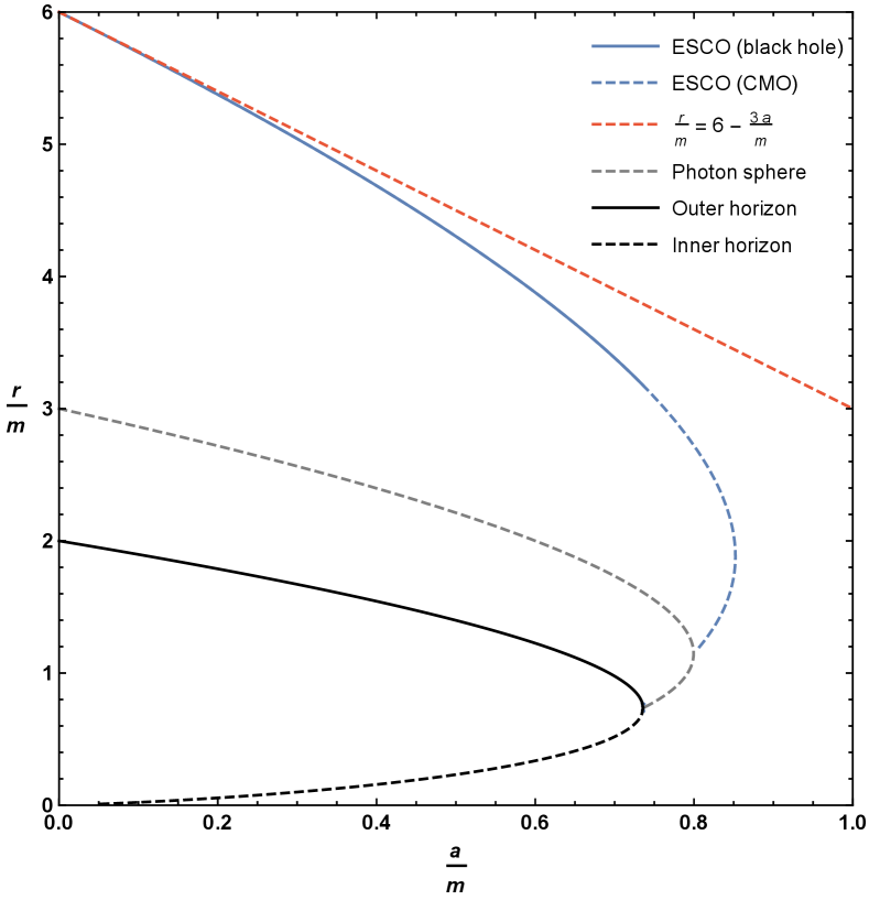
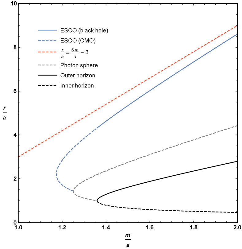
Plots of the boundary implied by equation (4.10), or equivalently (4.15), can be seen in Figure 4. As for the photon sphere, we have the interesting result that the extension of the ESCO to horizonless compact massive objects results in up to two possible ESCO locations for fixed values of $a$ and $m$ . Perhaps unexpectedly, the curve of ESCOs does not terminate at the horizon — it terminates once it hits the curve of circular photon orbits at a very special point. Let us now turn to the detailed analysis of both the qualitative behaviour and the various turning points presented in Figures 4 and 5. Note that where the ESCO is single-valued it is an ISCO (innermost stable circular orbit). Where the ESCO is double-valued the upper branch is an ISCO and the lower branch is an OSCO (outermost stable circular orbit) [71].

4.2.1 Perturbative analysis (small $a$ )

Let us first investigate the existence region perturbatively for small $a$ . We have

L_{c}(r_{c},m,a)^{2}={mr_{c}^{2}\over r_{c}-3m}-{2mr_{c}(r_{c}-m)\over(r_{c}-3m)^{2}}\;a+\mathcal{O}(a^{2}).

(4.16)

Note that this approximation diverges at the Schwarzschild photon sphere $r=3m$ .

So for small $a$ the boundary for the region of existence of timelike circular orbits is still $r=3m$ .

Now investigate the stability region perturbatively for small $a$ . Rearranging equation (4.10) we see

r_{c}={6m(r_{c}^{2}-ar_{c}+a^{2}/3)\mathrm{e}^{-a/r_{c}}\over r_{c}^{2}+ar_{c}-a^{2}}=6m\left(1-{3a\over r_{c}}+{\mathcal{O}}(a^{2})\right).

(4.17)

Thence

r_{c}=6m-3a+{\mathcal{O}}(a^{2}).

(4.18)

Which sensibly reproduces the Schwarzschild ISCO to lowest order in $a$ , and explains the asymptote in Figure 4 (b).

Furthermore, for small $a$ , substituting $L_{c}(r_{c})$ into $V^{\prime\prime}_{-1}(L,r_{c})$ and expanding

V_{-1}^{\prime\prime}(r_{c})={2m(r_{c}-6m)\over r_{c}^{3}(r_{c}-3m)}+{4m^{2}(7r_{c}-15m)\over r^{4}(r_{c}-3m)^{2}}\;a+{\mathcal{O}}(a^{2})

(4.19)

Demanding that this quantity be zero self-consistently yields $r_{c}=6m-3a+{\mathcal{O}}(a^{2})$ .

4.2.2 Non-perturbative analysis

We have already seen that, defining $w=r_{c}/a$ and $z=m/a$ , the curve describing the boundary of the region of stable timelike circular orbits can be rewritten as

2z(3w^{2}-3w+1)\mathrm{e}^{-1/w}=w(w^{2}+w-1).

(4.20)

Thence

z={w(w^{2}+w-1)\mathrm{e}^{1/w}\over 2(3w^{2}-3w+1)}.

(4.21)

Let us look for the turning points of $z(w)$ . The derivative is

{\differential z\over\differential w}={(w-1)(3w^{4}-6w^{3}-3w^{2}+4w-1)\mathrm{e}^{1/w}\over 2w(3w^{2}-3w+1)^{2}}.

(4.22)

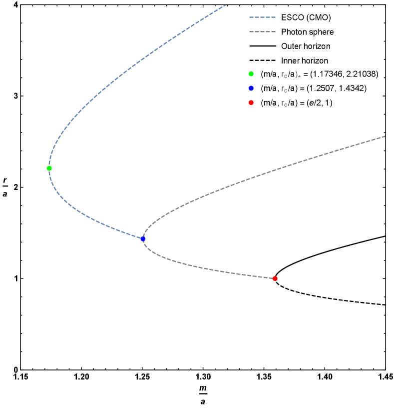
There is one obvious local extrema at $w=1$ , corresponding to $z=\mathrm{e}/2$ . Physically this corresponds to the point where inner and outer horizon merge and become extremal — but from inspection of Figure 4, the descriptive plots of Figure 5, and the zoomed-in plots of Figure 6, we see that the curve of ESCOs hits the photon orbit (and becomes unphysical) before getting to this point. In terms of the variables used when plotting Figures 4–6 this unphysical (from the point of view of ESCOs) point corresponds to

(r_{c}/a,m/a)_{*}=(1,\mathrm{e}/2)\qquad(r_{c}/m,a/m)_{*}=(2/\mathrm{e},2/\mathrm{e}).

(4.23)

The other local extrema is located at the only physical root of the quartic polynomial

3w^{4}-6w^{3}-3w^{2}+4w-1=0.

(4.24)

While this can be solved analytically, the results are too messy to be enlightening and so we resort to numerics. Two roots are complex, one is negative, the only physical root is $w=2.210375896...$ , corresponding to $z=1.173459017...$ . Physically this implies that the ESCO curve should exhibit a non-trivial local extremum — and from inspection of Figure 4 we see that the curve of ESCOs does indeed have a local extremum at this point. In terms of the variables used when plotting Figure 4 this extremal point corresponds to

(r_{c}/a,m/a)_{*}=(2.210375896,1.173459017),

(4.25)

and

(r_{c}/m,a/m)_{*}=(1.883641323,0.8521814444).

(4.26)

4.3 Intersection of ESCO and photon sphere

We can rewrite the curve for the loci of the photon spheres (3.4) as

\mathrm{e}^{-1/w}z={w^{2}\over(3w-1)}.

(4.27)

Similarly, for the loci of ESCOs rewrite (4.21) as

\mathrm{e}^{-1/w}z={w(w^{2}+w-1)\over 2(3w^{2}-3w+1)}.

(4.28)

These curves cross at

{w\over(3w-1)}={(w^{2}+w-1)\over 2(3w^{2}-3w+1)}.

(4.29)

That is, at

(w-1)(3w^{2}-5w+1)=0,

(4.30)

with explicit roots at

1,\quad{5\pm\sqrt{13}\over 6}.

(4.31)

The physically relevant root is $w={5+\sqrt{13}\over 6}=1.434258546...$ , which was where we previously determined that the photon sphere became stable, and at the point where the curve of photon spheres maximized the value of $z=m/a$ .

4.4 Explicit result for the angular momentum

We can rewrite the curve for the angular momentum (4.4) as

L_{c}^{2}=a^{2}\left(\mathrm{e}^{-1/w}z\;w^{2}(w-1)\over w^{2}-\mathrm{e}^{-1/w}z(3w-1)\right).

(4.32)

Similarly, for the loci of ESCOs we can rewrite (4.21) as

\mathrm{e}^{-1/w}z={w(w^{2}+w-1)\over 2(3w^{2}-3w+1)}.

(4.33)

We then substitute this into back into $L_{c}$ :

L_{c}^{2}=a^{2}\;{w^{2}(w^{2}+w-1)\over 3w^{2}-5w+1}.

(4.34)

This has a pole at $w={5+\sqrt{13}\over 6}=1.434258546...$ , and is then positive and finite for all $w>{5+\sqrt{13}\over 6}$ . (Of course the point $w={5+\sqrt{13}\over 6}$ on the ESCO curve is exactly where the ESCO curve hits the photon curve, so we would expect the angular momentum to go to infinity there.) Asymptotically for large $r$ (large $w=r_{c}/a$ ) we have $L_{c}^{2}\sim a^{2}w^{2}/3$ and $m/a=z\sim w/6$ , so $L_{c}^{2}\sim 2mr_{c}$ as expected from the large-distance Newtonian limit.

4.5 Summary

Overall, we see that the boundary of the stability region for timelike circular orbits is rather complicated. In terms of the variable $w=r_{c}/a$ :

•
For $w\in({5+\sqrt{13}\over 6},\infty)$ we have an ESCO.
This ESCO then subdivides as follows:
- –
  
  For $w\in(2.210375896,\infty)$ we have an ISCO.
- –
  
  For $w\in({5+\sqrt{13}\over 6},2.210375896)$ we have an OSCO.
•

For $w\in(1,{5+\sqrt{13}\over 6})$ the stability region is bounded by a stable photon orbit.
•

The line $w=1$ bounds the stability and existence region for timelike circular orbits from below.

This is considerably more complicated than might reasonably have been expected.

5 Conclusions

In this work we have investigated astrophysically observable quantities of a specific novel regular black hole model based on an asymptotically Minkowski core [62, 63]: Specifically we have investigated the photon sphere and ESCO. The spacetime under consideration is an example of a black hole mimicker. For the regular black hole model, both the photon sphere and the ESCO exist and are located outside of the outer horizon, and so (at least in theory) could be astrophysically observable. The analysis of the photon sphere and ESCO was extended to horizonless compact massive objects, leading to the surprising results that for fixed values of $m$ and $a$ , up to two possible photon sphere and up to two possible ESCO locations exist in our model spacetime; and that the very existence of the photon sphere and ESCO depends explicitly on the ratio $a/m$ . Somewhat unexpectedly, due to the effectively repulsive nature of gravity in the region near the core, we have found some situations in which the photon orbits are stable, and some situations where the ESCOs are OSCOs rather than ISCOs. There is a rich phenomenology here that is significantly more complex than for the Schwarzschild spacetime.

Acknowledgements

TB was supported by a Victoria University of Wellington MSc scholarship, and was also indirectly supported by the Marsden Fund, via a grant administered by the Royal Society of New Zealand.
AS acknowledges financial support via a PhD Doctoral Scholarship provided by Victoria University of Wellington. AS is also indirectly supported by the Marsden fund, via a grant administered by the Royal Society of New Zealand.
MV was directly supported by the Marsden Fund, via a grant administered by the Royal Society of New Zealand.

References

[1] K. Schwarzschild, “Über das Gravitationsfeld eines Massenpunktes nach der Einsteinschen Theorie”, Sitzungsberichte der Königlich Preussischen Akademie der Wissenschaften 7 (1916) 189. Free online version.
[2] H. Reissner, “Über die Eigengravitation des elektrischen Feldes nach der Einsteinschen Theorie”, Annalen der Physik 50 (1916) 106. Free online version.
[3] H. Weyl, “Zur Gravitationstheorie”, Annalen der Physik 54 (1917) 117.
Free online version.
[4] G. Nordström, “On the Energy of the Gravitational Field in Einstein’s Theory”, Verhandl. Koninkl. Ned. Akad. Wetenschap.,
Afdel. Natuurk., Amsterdam 24 (1918) 1201.
[5] R. Kerr, “Gravitational Field of a Spinning Mass as an Example of Algebraically Special Metrics”, Phys. Rev. Lett. 11 (1963) 237.
[6] E. Newmann, E. Couch, K. Chinnapared, A. Exton, A. Prakash and R. Torrence, “Metric of a Rotating, Charged Mass”, J. Math. Phys. 6 (1965) 918.
[7] R. Kerr and A. Schild, “Republication of: A new class of vacuum solutions of the Einstein field equations”, Gen. Rel. and Grav. 41 (2009), 2485.
(Original paper published 1965.)
[8] M. Visser, “The Kerr spacetime: A brief introduction”, [arXiv:0706.0622 [gr-qc]]. Published in [9].
[9] D. L. Wiltshire, M. Visser and S. M. Scott,
The Kerr spacetime: Rotating black holes in general relativity,
(Cambridge University Press, Cambridge, 2009).
[10] J. Baines, T. Berry, A. Simpson and M. Visser,
“Unit-lapse versions of the Kerr spacetime”, [arXiv:2008.03817 [gr-qc]].
[11] J. Baines, T. Berry, A. Simpson and M. Visser,
“Painleve-Gullstrand form of the Lense-Thirring spacetime,”
[arXiv:2006.14258 [gr-qc]].
[12] P. C. Vaidya, “The External Field of a Radiating Star in General Relativity”, Current Sci. (India) 12 (1943) 183.
[13] P. C. Vaidya, “The external field of a radiating star”,
Proc. Indian Acad. Sci. 33 (1951) 264.
[14] P. C. Vaidya, “Nonstatic solutions of Einstein’s field equations for spheres of fluids radiating energy” Phys. Rev. 83 (1951) 10.
[15] X. Calmet, “Quantum Aspects of Black Holes”, Springer Int. Pub. (2015).
[16] X. Calmet and B. K. El-Menoufi,
“Quantum corrections to Schwarzschild black hole”,
Eur. Phys. J. C 77 (2017) 243. [arXiv:1704.00261 [hep-th]].
[17] D. I. Kazakov and S. N. Solodukhin,
“On quantum deformation of the Schwarzschild solution”,
Nuc. Phys. B 429 (1994) 153. [arXiv:hep-th/9310150].
[18] A. F. Ali and M. M. Khalil, “Black hole with quantum potential”,
Nuc. Phys. B 909 (2016) 173. [arXiv:1509.02495 [gr-qc]].
[19] J. M. Bardeen, “Non-singular general-relativistic gravitational collapse”, in Proceedings of International Conference GR5, Tbilisi, U.S.S.R. (1968).
[20] S. A. Hayward, “Formation and Evaporation of Nonsingular Black Holes”,
Phys. Rev. Lett. 96 (2006) 031103. [arXiv:gr-qc/0506126].
[21] V. P. Frolov, “Information loss problem and a ‘black hole’ model with a closed apparent horizon”, J. High Energ. Phys. 2014 (2014). [arXiv:1402.5446 [hep-th]].
[22] S. Ansoldi, “Spherical black holes with regular center: a review of existing models including a recent realization with Gaussian sources”, (2008).
[arXiv:0802.0330 [gr-qc]].
[23] R. Carballo-Rubio, F. Di Filippo, S. Liberati, C. Pacilio and M. Visser,
“On the viability of regular black holes”, J. High Energ. Phys. 2018 (2018). [arXiv:1805.02675 [gr-qc]].
[24] M Morris and K. S. Thorne, “Wormholes in spacetime and their use for interstellar travel: A tool for teaching General Relativity”, Am. J. Phys. 56 (1988) 395.
[25] M. S. Morris, K. S. Thorne and U. Yurtsever, “Wormholes, Time Machines, and the Weak Energy Condition?”, Phys. Rev. Lett. 61 (1988) 1446.
[26] M. Visser, “Lorentzian Wormholes: From Einstein to Hawking”,
AIP press [now Springer], New York (1995).
[27] M. Visser, “Traversable wormholes: Some simple examples”,
Phys. Rev. D 39 (1989) 3182. [arXiv:0809.0907 [gr-qc]].
[28] M. Visser, “Traversable wormholes from surgically modified Schwarzschild space-times”, Nucl. Phys. B 328 (1989), 203-212 doi:10.1016/0550-3213(89)90100-4 [arXiv:0809.0927 [gr-qc]].
[29] M. Visser, “Wormholes, Baby Universes and Causality,” Phys. Rev. D 41 (1990), 1116 doi:10.1103/PhysRevD.41.1116
[30] M. Visser, S. Kar and N. Dadhich, “Traversable wormholes with arbitrarily small energy condition violations”, Phys. Rev. Lett. 90 (2003), 201102 doi:10.1103/PhysRevLett.90.201102 [arXiv:gr-qc/0301003 [gr-qc]].
[31] M. Visser, “From wormhole to time machine: Comments on Hawking’s chronology protection conjecture,” Phys. Rev. D 47 (1993), 554-565 doi:10.1103/PhysRevD.47.554 [arXiv:hep-th/9202090 [hep-th]].
[32] S. Kar, N. Dadhich and M. Visser, “Quantifying energy condition violations in traversable wormholes”, Pramana 63 (2004), 859-864 doi:10.1007/BF02705207 [arXiv:gr-qc/0405103 [gr-qc]].
[33] E. Poisson and M. Visser, “Thin shell wormholes: Linearization stability”,
Phys. Rev. D 52 (1995), 7318-7321 doi:10.1103/PhysRevD.52.7318 [arXiv:gr-qc/9506083 [gr-qc]].
[34] J. G. Cramer, R. L. Forward, M. S. Morris, M. Visser, G. Benford and G. A. Landis, “Natural wormholes as gravitational lenses,” Phys. Rev. D 51 (1995), 3117-3120 doi:10.1103/PhysRevD.51.3117 [arXiv:astro-ph/9409051 [astro-ph]].
[35] N. Dadhich, S. Kar, S. Mukherji and M. Visser, “ $R=0$ space-times and selfdual Lorentzian wormholes,” Phys. Rev. D 65 (2002), 064004 doi:10.1103/PhysRevD.65.064004 [arXiv:gr-qc/0109069 [gr-qc]].
[36] P. Boonserm, T. Ngampitipan, A. Simpson, and M. Visser,
“The exponential metric represents a traversable wormhole”,
Phys. Rev. D 98 (2018) 084048. [arXiv:1805.03781 [gr-qc]].
[37] A. Simpson and M. Visser, “Black-bounce to traversable wormhole”,
JCAP 1902 (2019) 042. [arXiv:1812.07114 [gr-qc]].
[38] A. Simpson, P. Martín-Moruno and M. Visser, “Vaidya spacetimes, black-bounces, and traversable wormholes,” Class. Quant. Grav. 36 (2019) no.14, 145007 doi:10.1088/1361-6382/ab28a5 [arXiv:1902.04232 [gr-qc]].
[39] F. S. N. Lobo, A. Simpson and M. Visser, “Dynamic thin-shell black-bounce traversable wormholes”, Phys. Rev. D 101 (2020) no.12, 124035 doi:10.1103/PhysRevD.101.124035 [arXiv:2003.09419 [gr-qc]].
[40] P. O. Mazur and E. Mottola, “Gravitational vacuum condensate stars”,
Proceedings of the National Academy of Sciences 101 (2004) 9545.
[41] P. O. Mazur and E. Mottola,
“Gravitational Condensate Stars: An Alternative to Black Holes”, (2001).
[arXiv:0109035 [gr-qc]]
[42] M. Visser and D. Wiltshire, “Stable gravastars: An alternative to black holes?”, Class. Quant. Grav. 21 (2004) 1135. [arXiv:gr-qc/0310107].
[43] C. Cattoën, T. Faber and M. Visser, “Gravastars must have anisotropic pressures,” Class. Quant. Grav. 22 (2005), 4189-4202 doi:10.1088/0264-9381/22/20/002 [arXiv:gr-qc/0505137 [gr-qc]].
[44] F. S. N. Lobo, “Stable dark energy stars”, Class. Quant. Grav. 23 (2006) 1525. [arXiv:gr-qc/0508115].
[45] P. Martín-Moruno, N. Montelongo-García, F. S. N. Lobo and M. Visser, “Generic thin-shell gravastars,” JCAP 03 (2012), 034 doi:10.1088/1475-7516/2012/03/034 [arXiv:1112.5253 [gr-qc]].
[46] F. S. N. Lobo, P. Martín-Moruno, N. Montelongo-García and M. Visser, “Novel stability approach of thin-shell gravastars,” doi:10.1142/9789813226609_0221 [arXiv:1512.07659 [gr-qc]].
[47] P. Cunha, V.P., E. Berti and C. A. R. Herdeiro,
“Light-Ring Stability for Ultracompact Objects”,
Phys. Rev. Lett. 119 (2017) no.25, 251102 doi:10.1103/PhysRevLett.119.251102 [arXiv:1708.04211 [gr-qc]].
[48] P. Cunha, V.P. and C. A. R. Herdeiro,
“Stationary black holes and light rings”,
Phys. Rev. Lett. 124 (2020) no.18, 181101 doi:10.1103/PhysRevLett.124.181101 [arXiv:2003.06445 [gr-qc]].
[49] R. Carballo-Rubio, F. Di Filippo, S. Liberati and M. Visser, “Opening the Pandora’s box at the core of black holes,” Class. Quant. Grav. 37 (2020) no.14, 145005 doi:10.1088/1361-6382/ab8141 [arXiv:1908.03261 [gr-qc]].
[50] M. Visser, C. Barceló, S. Liberati and S. Sonego,
“Small, dark, and heavy: But is it a black hole?,”
PoS BHGRS (2008), 010 doi:10.22323/1.075.0010 [arXiv:0902.0346 [gr-qc]].
[51] M. Visser, “Physical observability of horizons,” Phys. Rev. D 90 (2014) no.12, 127502 doi:10.1103/PhysRevD.90.127502 [arXiv:1407.7295 [gr-qc]].
[52] R. Carballo-Rubio, F. Di Filippo, S. Liberati and M. Visser, “Phenomenological aspects of black holes beyond general relativity”, Phys. Rev. D 98 (2018) 124009. [arXiv:1809.08238 [gr-qc]].
[53] The Event Horizon Telescope Collaboration, “First M87 Event Horizon Telescope Results. I. The Shadow of the Supermassive Black Hole”, ApJL 875 (2019) L1. [arXiv:1906.11238 [astro-ph.GA]].
[54] The Event Horizon Telescope Collaboration, “First M87 Event Horizon Telescope Results. II. Array and Instrumentation”, ApJL 875 (2019) L2.
[arXiv:1906.11239 [astro-ph.GA]].
[55] The Event Horizon Telescope Collaboration, “First M87 Event Horizon Telescope Results. III. Data Processing and Calibration”, ApJL 875 (2019) L3. [arXiv:1906.11240 [astro-ph.GA]].
[56] The Event Horizon Telescope Collaboration, “First M87 Event Horizon Telescope Results. IV. Imaging the Central Supermassive Black Hole”, ApJL 875 (2019) L4. [arXiv:1906.11241 [astro-ph.GA]].
[57] The Event Horizon Telescope Collaboration, “First M87 Event Horizon Telescope Results. V. Physical Origin of the Asymmetric Ring”, ApJL 875 (2019) L5. [arXiv:1906.11242 [astro-ph.GA]].
[58] The Event Horizon Telescope Collaboration, “First M87 Event Horizon Telescope Results. VI. The Shadow and Mass of the Central Black Hole”, ApJL 875 (2019) L6. [arXiv:1906.11243 [astro-ph.GA]].
[59] See https://www.ligo.caltech.edu/page/detection-companion-papers for a collection of detection papers from LIGO.
See also https://pnp.ligo.org/ppcomm/Papers.html for a complete list of publications from the LIGO Scientific Collaboration and Virgo Collaboration.
[60] See, for example, wikipedia.org/List_of_gravitational_wave_observations for a list of current (May 2020) gravitational wave observations.
[61] E. Barausse, E. Berti, T. Hertog, S. A. Hughes, P. Jetzer, P. Pani, T. P. Sotiriou, N. Tamanini, H. Witek, K. Yagi, N. Yunes, et al.,
“Prospects for Fundamental Physics with LISA”,
Gen.Rel.Grav. 52 (2020) 8, doi:10.1007/s10714-020-02691-1.
[arXiv:2001.09793 [gr-qc]].
[62] A. Simpson and M. Visser,
“Regular black holes with asymptotically Minkowski cores”,
Universe 6 (2020) 8. [arXiv:1911.01020 [gr-qc]].
[63] T. Berry, F. S. N. Lobo, A. Simpson and M. Visser, “Thin-shell traversable wormhole crafted from a regular black hole with asymptotically Minkowski core”, Physical Review D (in press), [arXiv:2008.07046 [gr-qc]].
[64] H. Culetu, “On a regular modified Schwarzschild spacetime”,
arXiv:1305.5964 [gr-qc].
[65] H. Culetu, “On a regular charged black hole with a nonlinear electric source”,
Int. J. Theor. Phys. 54 (2015) no.8, 2855 doi:10.1007/s10773-015-2521-6 [arXiv:1408.3334 [gr-qc]].
[66] H. Culetu, “Nonsingular black hole with a nonlinear electric source”,
Int. J. Mod. Phys. D 24 (2015) no.09, 1542001. doi:10.1142/S0218271815420018
[67] H. Culetu, “Screening an extremal black hole with a thin shell of exotic matter”,
Phys. Dark Univ. 14 (2016) 1 doi:10.1016/j.dark.2016.07.004
[arXiv:1508.01102 [gr-qc]].
[68] E. L. B. Junior, M. E. Rodrigues and M. J. S. Houndjo,
“Regular black holes in $f(T)$ Gravity through a nonlinear electrodynamics source”, JCAP 1510 (2015) 060 doi:10.1088/1475-7516/2015/10/060
[arXiv:1503.07857 [gr-qc]].
[69] M. E. Rodrigues, E. L. B. Junior, G. T. Marques and V. T. Zanchin,
“Regular black holes in $f(R)$ gravity coupled to nonlinear electrodynamics”,
Phys. Rev. D 94 (2016) no.2, 024062
Addendum: [Phys. Rev. D 94 (2016) no.4, 049904] doi:10.1103/PhysRevD.94.024062, 10.1103/PhysRevD.94.049904
[arXiv:1511.00569 [gr-qc]].
[70] R. M. Corless, G. H. Gonnet, D. E. G. Hare, D. J. Jeffrey and D. E. Knuth,
“On the Lambert $W$ function”, Adv. Comput. Math. 5 (1996), 329-359 doi:10.1007/BF02124750
[71] P. Boonserm, T. Ngampitipan, A. Simpson and M. Visser, “Innermost and outermost stable circular orbits in the presence of a positive cosmological constant”, Phys. Rev. D 101 (2020) no.2, 024050 doi:10.1103/PhysRevD.101.024050 [arXiv:1909.06755 [gr-qc]].

Photon spheres, ISCOs, and OSCOs: Astrophysical observables for regular black holes with asymptotically Minkowski cores

Abstract

1 Introduction

2 Geodesics and the effective potential

3 Photon spheres

3.1 Existence of photon spheres

3.2 Stability versus instability for circular photon orbits

3.2.1 Perturbative analysis (small aa)

3.2.2 Non-perturbative analysis

3.3 Turning points

4 Timelike circular orbits

4.1 Existence of circular timelike orbits

4.2 Stability versus instability for circular timelike orbits

4.2.1 Perturbative analysis (small aa)

4.2.2 Non-perturbative analysis

4.3 Intersection of ESCO and photon sphere

4.4 Explicit result for the angular momentum

4.5 Summary

5 Conclusions

Acknowledgements

References

3.2.1 Perturbative analysis (small $a$ )

4.2.1 Perturbative analysis (small $a$ )