Physical Meaning of Principal Component Analysis for Lattice Systems with Translational Invariance

An unprecedented achievement of machine learning has brought physics into the realm of data-driven science. Like other successful applications of machine learning in physics [1, 2], principal component analysis (PCA) [3] for systems with phase transitions has attracted attention because it operates almost as an automated machine for identifying transition points, even without detailed information about the nature of the transitions [4, 5, 6, 7, 8].

A PCA study of phase transitions typically involves two steps. In the first step, which will be referred to as the data-preparation step, independent configurations are sampled using Monte Carlo simulations. The second step, which will be called the PCA step, analyzes the singular values of a matrix constructed by concatenating the configurations obtained in the data-preparation step (in the following presentation, we will actually consider positive matrices whose eigenvalues are the singular values in question). It is the largest singular value (that is, the principal component) that pinpoints a critical point and estimates a certain critical exponent [4, 5, 6, 7, 8].

The numerical observations clearly suggest that the principal component should be associated with the order parameter of a system in one way or another. In this Letter, we attempt to explain how the principal component is related with the order parameter. To be specific, we will find approximate expressions for all the singular values of matrices constructed in the PCA step. The expressions will be given for any $d$-dimensional lattice system with translational invariance. By the expressions, the connection between the principal component and the order parameter is immediately understood. In due course, we will argue that the more (data are collected in the data-preparation step), the better (the approximation).

We will first develop a theory for a one-dimensional lattice system with $L$ sites. A theory for higher dimensional systems will be easily come up with, once the one-dimensional theory is fully developed. Although we limit ourselves to hypercubic lattices, our theory can be easily generalized to other Bravais lattices.

Let us begin with the formal preparation for lattice systems. We assume that each site $n$, say, has a random variable $x_{n}$. Depending on the context, $x_{n}$ can be a binary number ($-1$ or $1$ for the Ising model, $0$ or $1$ for hard-core classical particles), a nonnegative integer (classical boson particles; see Ref. [9, 10] for a numerical method to simulate classical reaction-diffusion systems of bosons), a continuous vector (the $XY$ model, the Heisenberg model), or even a complex number ($e^{i\theta_{n}}$ in the $XY$ model, for instance). We assume periodic boundary conditions; $x_{n+L}=x_{n}$ in one dimension and a similar criterion in two or more dimensions. By $C$, we will denote a (random) configuration of a system. Denoting a column vector with a one in the $n$-th row and zeros in all other rows by $|n\rangle_{R}$ (the subscript $R$ is intended to mean “real” space), we represent a configuration as

$\displaystyle C\doteq\sum_{n=1}^{L}x_{n}|n\rangle_{R}.$

Obviously, $|n\rangle_{R}$’s form an orthonomal basis. To make use of the periodic boundary conditions, we set $|n+L\rangle_{R}=|n\rangle_{R}$.

By $P(C)$, we mean probability that the system is in configuration $C$ (in the case that $x_{n}$ takes continuous values, $P$ should be understood as probability density). Here, $P(C)$ is not limited to stationarity; $P(C)$ can be probability at a certain fixed time of a stochastic lattice model. For a later reference, we define “ensemble” average of a random variable $Y$ as

$$\langle Y\rangle=\sum_{C}Y(C)P(C),$$

where $Y(C)$ means a realization of $Y$ in configuration $C$ and $\sum$ should be understood as an integral if $P(C)$ is probability density.

When we write $C_{\alpha}$ for a certain configuration, $x_{n}$ in $C_{\alpha}$ will be denoted by $x_{n}^{(\alpha)}$. By translational invariance, we mean $P(C_{1})=P(C_{2})$ if configuration $C_{1}$ is related with configuration $C_{2}$ by $x_{n}^{(1)}=x_{n+m}^{(2)}$ for all $n$ and for a certain $m$.

Now we are ready to develop a formal theory. Let $N$ be a fixed positive integer and let $C_{\alpha}$’s be independent and identically distributed $N$ random configurations sampled from the common probability $P(C)$ ($\alpha=1,2,\ldots,N$). In practice, $C_{\alpha}$’s are prepared for in the data-preparation step.

For a later reference, we define an “empirical” average of a random variable Y as

$$[Y]_{N}:=\frac{1}{N}\sum_{\alpha=1}^{N}Y({C_{\alpha}}).$$

Unlike the ensemble average, the empirical average is a random variable. By the law of large numbers, $[Y]_{N}$ converges (at least in probability) to $\langle Y\rangle$, if exists, under the infinite $N$ limit. We define a centered configuration as

$$\overline{C}_{\alpha}:=\sum_{n}\left(x_{n}^{(\alpha)}-[x_{n}]_{N}\right)|n\rangle_{R}.$$

In the PCA step, main interest is in the spectral decomposition of an empirical second-moment matrix $M$ and an empirical covariance matrix $G$, defined as

$$M:=\frac{1}{N}\sum_{\alpha=1}^{N}C_{\alpha}C_{\alpha}^{\dagger},\quad G:=\frac{1}{N}\sum_{\alpha=1}^{N}\overline{C}_{\alpha}\overline{C}_{\alpha}^{\dagger}.$$

The elements of $M$ and $G$ can be written as ($1\leq n,m\leq L$)

	$\displaystyle M_{nm}$	$\displaystyle=\frac{1}{N}\sum_{\alpha=1}^{N}x^{(\alpha)}_{n}x^{(\alpha)*}_{m}=\left[x_{n}x_{m}^{*}\right]_{N},$
	$\displaystyle G_{nm}$	$\displaystyle=\frac{1}{N}\sum_{\alpha=1}^{N}\left(x^{(\alpha)}_{n}-[x_{n}]_{N}\right)\left(x^{(\alpha)}_{m}-[x_{m}]_{N}\right)^{*}$
		$\displaystyle=\left[\left(x_{n}-[x_{n}]_{N}\right)\left(x_{m}-[x_{m}]_{N}\right)^{*}\right]_{N},$

where the asterisk means complex conjugate. If $x_{n}$ is a vector as in the Heisenberg model, then the multiplications in the above would be replaced by inner products of two vectors. The periodic boundary conditions imply $M_{n+L,m}=M_{n,m+L}=M_{nm}$ and similar relations for $G$. Obviously, $M$ and $G$ are positive matrices. In what follows, we will denote the $r$-th largest eigenvalue of $M$ and $G$ by $\lambda_{r}^{M}$ and $\lambda_{r}^{G}$, respectively.

We will first find an approximate formula for $\lambda_{r}^{M}$. Once it is done, an approximate formula for $\lambda_{r}^{G}$ will be obtained immediately. Let us introduce a hermitian $L\times L$ matrix $S$ with elements

$\displaystyle S_{nm}=\begin{cases}E_{m-n},&m\geq n,\\ E_{n-m}^{*}&n>m\end{cases},\quad E_{j}:=\frac{1}{L}\sum_{n=1}^{L}M_{n,n+j}.$

Since $E_{L-j}=E_{j}^{*}$ by definition, $S$ is translationally invariant in that $S_{n+1,m+1}=S_{nm}$ for any pair of $n$ and $m$. Also note that $\operatorname{Tr}S=\operatorname{Tr}M=LE_{0}$.

Let $\hat{T}$ be a translation operator with $\hat{T}|n\rangle_{R}=|n+1\rangle_{R}$ for all $n$. Note that

$\displaystyle|k\rangle:=\frac{1}{\sqrt{L}}\sum_{n=1}^{L}\exp\left(i\frac{2\pi k}{L}n\right)|n\rangle_{R}$

for $k=0,1,2,\ldots,L-1$ is the eigenstate of $\hat{T}$ with the corresponding eigenvalue $\exp(-i2\pi k/L)$. Since $S$ is translationally invariant, we have $\hat{T}S=S\hat{T}$ and, accordingly, $|k\rangle$’s are also the eigenstates of $S$. Due to orthonormality $\langle k|k^{\prime}\rangle=\delta_{kk^{\prime}}$, the eigenvalues of $S$ are obtained by $\langle k|S|k\rangle$.

If $E_{j}$’s are real and nonnegative, which is the case if $x_{n}$’s are nonnegative real numbers, then we have, by the Perron-Frobenius theorem, the largest eigenvalue of $S$ as

	$\displaystyle\langle 0|S|0\rangle$	$\displaystyle=\sum_{j=0}^{L-1}E_{j}=\frac{1}{L}\sum_{j=0}^{L-1}\sum_{n=1}^{L}M_{n,n+j}$		(1)
		$\displaystyle=L\frac{1}{N}\sum_{\alpha=1}^{N}\left(\frac{1}{L}\sum_{n=1}^{L}x_{n}^{(\alpha)}\right)^{2}=L\left[\left(X_{1}\right)^{2}\right]_{N},$

where

$$X_{1}:=\frac{1}{L}\sum_{n=1}^{L}x_{n}$$

is a random variable, signifying a spatial average of $x$’s.

Now we move on to the eigenvalues of $M$. Let $\delta M:=M-S$. As $N$ increases, $M$ should become more and more translationally invariant in the sense that $M_{nm}-S_{nm}$, for any pair of $n$ and $m$, converges (presumably at least in probability) to zero under the infinite $N$ limit. Therefore, if $N$ is sufficiently large, $\delta M$ is very likely to be a small perturbation in comparison with $S$.

If $N$ is small or an atypical collection of $N$ configurations (unfortunately) happens to be sampled, however, $\delta M$ may not be considered a perturbation. For example, if $N=1$ and $x_{n}$’s are nonnegative, $M$ is a rank one matrix with eigenstate $C_{1}$ and the only nonzero eigenvalue of $M$ is $C_{1}^{\dagger}C_{1}=LE_{0}$, while the largest eigenvalue of $S$ is still given in Eq. (1). In the case that $x_{n}$ only assumes zero or one and $[X_{1}]_{1}\ll 1$, $\delta M$ cannot be regarded as a perturbation, because $E_{0}=[X_{1}]_{1}\gg[X_{1}]_{1}^{2}=[(X_{1})^{2}]_{1}$. Note, however, that if $[X_{1}]_{1}\simeq 1$ in the above example, then $\delta M$ even for $N=1$ is still a perturbation.

In many cases (see below), $\langle X_{1}\rangle$ is the order parameter. If this is indeed the case, then the principal component of $M$ for $N=1$ is just the order parameter, especially for large $L$, and, therefore, can still be used to study phase transitions, although PCA for $N=1$ is practically unnecessary.

In the case that $\delta M$ indeed can be treated as a perturbation, the Rayleigh-Schrödinger perturbation theory in quantum mechanics (up to the first order) gives the approximate eigenvalues of $M$ as

	$\displaystyle\tau_{k}^{M}$	$\displaystyle:=\langle k|M|k\rangle=\frac{1}{L}\sum_{nm}e^{-i2\pi kn/L}M_{nm}e^{i2\pi km/L}$
		$\displaystyle=\frac{1}{L}\sum_{nm}\left[e^{-i2\pi kn/L}x_{n}e^{i2\pi km/L}x_{m}^{*}\right]_{N}=\left[\left|\tilde{X}_{k}\right|^{2}\right]_{N},$

where

$$\tilde{X}_{k}:=\frac{1}{\sqrt{L}}\sum_{n=1}^{L}e^{-i2\pi kn/L}x_{n}$$

is the $k$-th mode of Fourier transform of $x_{n}$, with $\tilde{X}_{0}=\sqrt{L}X_{1}$. That is, all the eigenvalues of $M$ are approximated by the empirical average of the (square of) moduli of Fourier modes when $N$ is sufficiently large. Following the same discussion as above, we can get the approximate eigenvalues of $G$ as $\tau_{k}^{G}:=\langle k|G|k\rangle$. It is straightforward to get

$\displaystyle\tau_{k}^{G}=\left[\left|\tilde{X}_{k}-[\tilde{X}_{k}]_{N}\right|^{2}\right]_{N}.$

Since $\tilde{X}_{k}^{*}=\tilde{X}_{L-k}$, we have $\tau_{k}^{M}=\tau_{L-k}^{M}$ and $\tau_{k}^{G}=\tau_{L-k}^{G}$.

Let $(k_{1},k_{2},\ldots,k_{L})$ be a permutation of $(0,1,\ldots,L-1)$ such that $\tau_{k_{r}}^{M}\geq\tau_{k_{r+1}}^{M},$ for all $1\leq r\leq L-1$, then we have $\lambda_{r}^{M}\approx\tau_{k_{r}}^{M}$. A similar rearrangement of $\tau_{k}^{G}$ will give $\lambda_{r}^{G}\approx\tau_{k_{r}}^{G}$. Therefore, one can find all the eigenvalues of $M$ and $G$ approximately, already in the data-preparation step. Furthermore, we would like to emphasize once again that $\tau_{k_{r}}^{M,G}$ should converge (at least in probability) to $\lambda_{r}^{M,G}$ under the limit $N\rightarrow\infty$.

If the system has the translational invariance, the law of large numbers gives

$$\lim_{N\rightarrow\infty}[x_{n}]_{N}=\lim_{N\rightarrow\infty}[x_{m}]_{N},$$

for all $1\leq n,m\leq L$ and, accordingly,

$$\lim_{N\rightarrow\infty}[\tilde{X}_{k}]_{N}=0,$$

for nonzero $k$. Therefore, we have

$$\lim_{N\rightarrow\infty}\tau_{k}^{G}=\lim_{N\rightarrow\infty}\tau_{k}^{M},$$

for nonzero $k$. Hence, only $\tau_{0}^{G}$ and $\tau_{0}^{M}$ may remain different as one collects more and more samples, while $\tau_{k}^{G}$ and $\tau_{k}^{M}$ become closer and closer to each other as $N$ gets larger and larger.

For a $d$-dimensional system with $L_{\ell}$ sites along the $\ell$-th direction, the result for the one-dimensional system can be easily generalized, to yield approximate expressions for eigenvalues of $M$ and $G$ as

	$\displaystyle\tau_{\vec{p}}^{M}$	$\displaystyle:=\left[\left|\tilde{X}_{\vec{p}}\right|^{2}\right]_{N},\quad\tau_{\vec{p}}^{G}:=\left[\left|\tilde{X}_{\vec{p}}-\left[\tilde{X}_{\vec{p}}\right]_{N}\right|^{2}\right]_{N},$		(2)
	$\displaystyle\tilde{X}_{\vec{p}}$	$\displaystyle:=\frac{1}{\sqrt{L}}\sum_{\vec{r}}e^{-i\vec{p}\cdot\vec{r}}x_{\vec{r}},\quad\vec{r}=(n_{1},\ldots,n_{d}),$

where $\vec{r}$ is the lattice vector with $1\leq n_{\ell}\leq L_{\ell}$ ($\ell=1,2,\ldots,d$),

$$\vec{p}=2\pi\left(\frac{k_{1}}{L_{1}},\ldots,\frac{k_{d}}{L_{d}}\right)$$

is the reciprocal lattice vector (of the $d$-dimensional hypercubic lattice) with $0\leq k_{\ell}<L_{\ell}$ ($\ell=1,2,\ldots,d$), and $L:=\prod_{\ell=1}^{d}L_{\ell}$ is the total number of sites.

If $X_{1}$ happens to be an order parameter of a phase transition, $\tau_{0}^{M}/L$ is just square of the order parameter and $\tau_{0}^{G}$ is the fluctuation of the order parameter. Here, the subscript $0$ is a shorthand notation for the zero reciprocal lattice vector $(0,0,\ldots,0)$. Accordingly, under the infinite $L$ limit, $\tau_{0}^{M}/L$ or, equivalently, $\lambda_{1}^{M}/L$, should play the role of an order parameter and $\tau_{0}^{G}$ and, equivalently, the principal component $\lambda_{1}^{G}$ should diverge at the critical point. For example, in the Ising model, $X_{1}=\tilde{X}_{0}/\sqrt{L}$ is the magnetization $\mathcal{M}$ and, therefore, $\tau_{0}^{M}\approx L\langle\mathcal{M}^{2}\rangle$ and $\tau_{0}^{G}\approx L(\langle\mathcal{M}^{2}\rangle-\langle\mathcal{M}\rangle^{2})$ for sufficiently large $N$. This obviously explains why PCA works.

To support the above theory numerically, we apply PCA to the one and two dimensional contact process (CP) [11]. The CP is a typical model of absorbing phase transitions (for a review, see, e.g., Ref [12, 13]). In the CP, each site is either occupied by a particle ($x_{n}=1$) or vacant ($x_{n}=0$). No multiple occupancy is allowed. Each particle dies with rate $p$ and branches one offspring to randomly chosen one of its nearest neighbor sites with rate $1-p$. If the target site is already occupied in the branching attempt, no configuration change occurs. Note that $\langle X_{1}\rangle$ is the order parameter and $\tau_{0}^{M}$ should converge to $L\langle X_{1}^{2}\rangle$ for all $t$ under the infinite $N$ limit.

In the data-preparation step, we simulated the one dimensional CP (at $p=0.232$) with $L=64$ and the two dimensional CP (at $p=0.29$) with $L_{1}=L_{2}=8$. For all cases, we use the fully occupied initial condition ($x_{n}=1$ for all $n$), which ensures the translational invariance at all time. We collected $10^{4}$ independent configurations at $t=40$. In the PCA step, we constructed $M$’s and $G$’s with different numbers of configurations, which were numerically diagonalized.

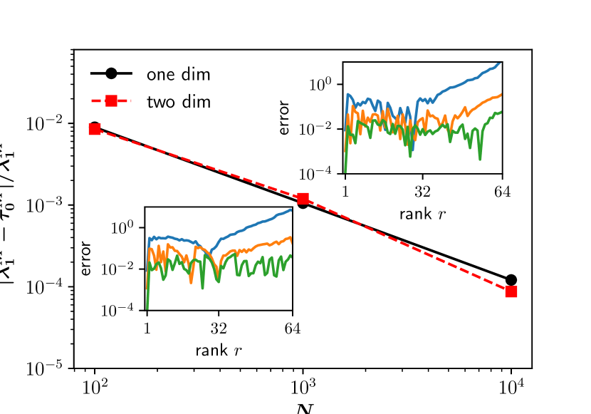
In Fig. 1, we depict the relative error of $\tau_{0}^{M}$, defined as $|\lambda_{1}^{M}-\tau_{0}^{M}|/\lambda_{1}^{M}$, for the one-dimensional and the two-dimensional CPs against $N$ on a double-logarithmic scale. Indeed, the error gets smaller with $N$ in any dimensions. Quantitatively, the relative error decreases as $O(1/N)$, which should be compared with $\tau_{0}^{M}-L\langle X_{1}^{2}\rangle=O(1/\sqrt{N})$ due to the central limit theorem.

Since our theory is not limited to the largest eigenvalue, we also study relative errors of other eigenvalues. In the inset of Fig. 1, we depict $|\lambda_{r}^{M}-\tau_{k_{r}}^{M}|/\lambda_{r}^{M}$ vs $r$ ($r$ is the rank of the values) for the one-dimensional (upper panel) and the two-dimensional (lower panel) CPs. Again, the errors indeed tend to decrease with $N$.

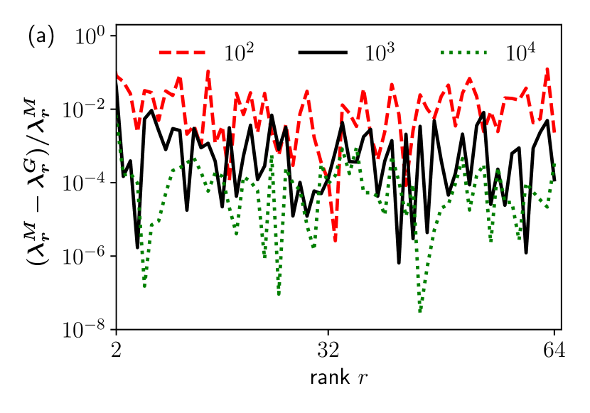
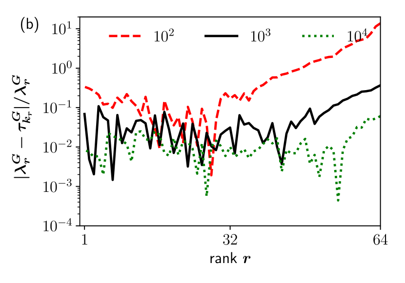
In Fig. 2(a), we compare $\lambda^{M}_{r}$ and $\lambda_{r}^{G}$ for $r\geq 2$. As expected, the difference of the eigenvalues except the largest one tends to approach zero as $N$ increases. In Fig. 2(b), we compare $\tau_{k_{r}}^{G}$ and $\lambda_{r}^{G}$, which also supports that $\tau_{k}^{G}$’s with appropriate ordering indeed tend to become better and better approximations for $\lambda_{r}^{G}$, as $N$ increases. A similar behavior is also observed in two dimensions (details not shown here). The example of the CP supports the validity of our theory.

For a sufficiently large system, a typical configuration of a translationally invariant system is expected to be homogeneous and, therefore, it is likely that $\tilde{X}_{k}$ for $k\neq 0$ converges (presumably at least in probability) to zero under the infinite $L$ limit. Hence, except the $k=0$ mode, all other eigenvalues goes to zero as $L\rightarrow\infty$, which is consistent with numerical observations in the literature (see, for example, Fig. 1 of Ref. [4] that shows the decrease of non-principal components with $N$).

In all the examples in the above, the largest eigenvalue $\lambda_{1}^{M}$ happens to be approximated by $\tau_{0}^{M}$. However, this needs not be the case for every stochastic lattice model. For example, let us consider the Kawasaki dynamics [14] of the two dimensional Ising model with zero magnetization. In this case, both $X_{1}$ and $\tau_{0}^{M}$ are by definition zero, regardless of $N$. Therefore, $\lambda_{1}^{M}$ should be a Fourier mode with nonzero reciprocal lattice vector. Since the Ising model is also isotropic, we must have

$$\lim_{N\rightarrow\infty}\left(\tau_{\vec{p}_{1}}^{M}-\tau_{\vec{p}_{2}}^{M}\right)=0,\,\vec{p}_{1}:=\frac{2\pi}{L}(k,0),\,\vec{p}_{2}:=\frac{2\pi}{L}(0,k),$$

for any integer $k$. In case the Fourier mode with the smallest nonzero $|\vec{p}|$ gives the $\lambda_{1}^{M}$ in the infinite $N$ limit, there should be $4$ significant eigenvalues of $M$ for finite $N$, which was indeed observed in Fig. 4 of Ref. [4].

To conclude, Eq. (2) for approximating all the eigenvalues of the empirical second-moment matrix $M$ and the empirical covariance matrix $G$ clearly indicates the relation between the principal component and the order parameter of the system in question and explains why PCA has to be working. Moreover, Eq. (2) can reduce computational efforts, because it can be calculated already in the data-preparation step; there is no need of the PCA step for PCA if the system has the translational invariance.

Since our theory heavily relies on the translational invariance, Eq. (2) is unlikely to be applicable to a system without the translational invariance such as a system with quenched disorder, a system on a scale-free network, and so on. It would be an interesting future research topic to check whether PCA for a system without the translational invariance still be of help and, if so, to answer why.

This work was supported by the National Research Foundation of Korea (NRF) grant funded by the Korea government (Grant No. RS-2023-00249949).

References

- Mehta et al. [2019] P. Mehta, M. Bukov, C.-H. Wang, A. G. Day, C. Richardson, C. K. Fisher, and D. J. Schwab, A high-bias, low-variance introduction to machine learning for physicists, Phys. Rep. 810, 1 (2019).
- Carleo et al. [2019] G. Carleo, I. Cirac, K. Cranmer, L. Daudet, M. Schuld, N. Tishby, L. Vogt-Maranto, and L. Zdeborová, Machine learning and the physical sciences, Rev. Mod. Phys. 91, 045002 (2019).
- Jolliffe [2002] I. T. Jolliffe, Principal Component Analysis (Springer, New York, 2002).
- Wang [2016] L. Wang, Discovering phase transitions with unsupervised learning, Phys. Rev. B 94, 195105 (2016).
- Carrasquilla and Melko [2017] J. Carrasquilla and R. G. Melko, Machine learning phases of matter, Nat. Phys. 13, 431 (2017).
- Hu et al. [2017] W. Hu, R. R. P. Singh, and R. T. Scalettar, Discovering phases, phase transitions, and crossovers through unsupervised machine learning: A critical examination, Phys. Rev. E 95, 062122 (2017).
- Sale et al. [2022] N. Sale, J. Giansiracusa, and B. Lucini, Quantitative analysis of phase transitions in two-dimensional models using persistent homology, Phys. Rev. E 105, 024121 (2022).
- Muzzi et al. [2024] C. Muzzi, R. S. Cortes, D. S. Bhakuni, A. Jelić, A. Gambassi, M. Dalmonte, and R. Verdel, Principal component analysis of absorbing state phase transitions (2024), arXiv:2405.12863 [cond-mat.stat-mech] .
- Park [2005] S.-C. Park, Monte carlo simulations of bosonic reaction-diffusion systems, Phys. Rev. E 72, 036111 (2005).
- Park [2006] S.-C. Park, Monte Carlo simulations of bosonic reaction-diffusion systems and comparison to Langevin equation description, Eur. Phys. J. B 50, 327 (2006).
- Harris [1974] T. E. Harris, Contact interactions on a lattice, Ann. Prob. 2, 969 (1974).
- Hinrichsen [2000] H. Hinrichsen, Non-equilibrium critical phenomena and phase transitions into absorbing states, Adv. Phys. 49, 815 (2000).
- Ódor [2004] G. Ódor, Universality classes in nonequilibrium lattice systems, Rev. Mod. Phys. 76, 663 (2004).
- Kawasaki [1966] K. Kawasaki, Diffusion constants near the critical point for time-dependent Ising models. I, Phys. Rev. 145, 224 (1966).