Physics-constrained Active Learning for Soil Moisture Estimation and Optimal Sensor Placement

Physics-informed machine learning (PIML) is a powerful tool that incorporates the prior knowledge of physical laws and the actual sensor observations in a data-driven framework. As a result, PIML can overcome the low data availability issue that would limit the capability of most machine learning models. PIML incorporates known physical laws as constraints during training, enhancing its ability to generalize beyond data, improve interpretability, and guide predictions in accordance with underlying physical laws. For example, Raissi et al. [17] built a physics-informed neural network (PINN) framework that integrates well-established physics laws with deep learning to suppress the model dependence on training data. The efficacy of PINN has already been verified in numerous physical systems, such as the fluid dynamics [18], solid mechanics [19, 20], heat transfer [21], and biological systems [11, 22].

In terms of root-zone soil moisture estimation, most existing agro-hydrological models are based on the Richards equation (RE) [23], which captures irrigation, precipitation, evapotranspiration, runoff, and drainage dynamics in soil. Recently, researchers have investigated the application of PINNs to model soil moisture dynamics by incorporating the RE. Notably, Tartakovsky et al. [24] were one of the first teams to utilize PINNs to derive the hydraulic conductivity function in unsaturated homogeneous soil using pressure head data based on the 2D RE. Banbai et al. [25] embedded RE into PINN to inversely learn the soil moisture dynamics only from soil sensor measurements without engaging any pre-assumptions on soil hydraulic functions and realize a free-form representation of constitutive relationships. Depina [26] inherited and extended Banbai et al.’s work and utilized PINN to investigate the 1D solutions of the RE that adopts the van Genuchten constitutive model, which allows a simpler neural network structure for pressure head estimation. More recently, Haruzi et al. [27] proposed a PINN model with non-invasive geometric data to simulate 2D water flow and solute transport. These studies mainly focus on the application of PINN in 1D or 2D soil systems. On the other hand, this work generalizes the predictive capabilities of PINNs to 3D soil systems. Meanwhile, integrating underlying physics (i.e., the RE) into deep neural networks can help reduce reliance on extensive sensor measurements, however, the performance of these predictive models still significantly depends on the volume and quality of training data [22].

As mentioned earlier, it is unaffordable and impractical to deploy sensors everywhere in the field. Conventional grid or random sampling strategies based on heuristics (ranging from 2 sensors/100 acres [28] to 20 sensors/acre [29]) are also arbitrary and ineffective. For in situ soil moisture sensing, more systematic sensor placement algorithms have been developed to better infer field-wide soil moisture profile from sparse sensor measurements. Wu et al. [30] used statistical clustering with the Gaussian process to find a coarse-grained monotonic ordering of locations in terms of the soil moisture content. Specifically, they classified the clusters based on the order of the mean and the number of sensors allocated to each cluster is decided based on the variance’s magnitude. Dursun et al. [31] developed a generic algorithm that iteratively refines soil moisture sensor locations. This algorithm works by continuously eliminating the least effective sensor position and replacing it with the most optimal candidate from the current iteration. Sahoo et al. [32] propose to estimate the soil moisture dynamics in agro-hydrological systems with the Kalman filter. They use the graphic approach with structural observability to identify the minimal number of sensors, followed by using the modal degree of observability to find their optimal placement. However, these optimal sensor placement approaches stem from either a statistical perspective or a graphical understanding. They did not consider the underlying physics rules to guide the search, which makes the selection devoid of fundamental physics insights.

The soil moisture dynamics are fundamentally governed by the Richards equation (RE) [23]. Without loss of generality of our P-DAL framework, we consider the scenarios where the sink term accounting for root water uptake is negligible. The resulting continuity equation that models the mass balance of water in a soil system is written as:

$$\frac{\partial\theta(\psi)}{\partial t}=-\nabla\cdot q$$

(1)

where $\theta$ is the volumetric water content in the soil (i.e., soil moisture), $\psi$ stands for the pressure head, $t$ denotes time, and $q$ represents the water flux. In addition to the continuity equation, the RE incorporates the Buckingham-Darcy law [33], which extends the traditional Darcy’s Law to account for the capillary forces in unsaturated soils. This is characterized by the relationship between $q$ and $\psi$:

$$q=-K(\psi)\cdot\nabla(\psi+z)$$

(2)

where $K$ is the hydraulic conductivity. By incorporating Buckingham-Darcy’s law of Eq. (2) into Eq. (1), the RE can be expressed as:

$$\frac{\partial\theta(\psi)}{\partial t}=\nabla\cdot(K(\psi)\nabla(\psi+z))$$

(3)

It is worth noting that the pressure head $\psi$ is a spatiotemporal variable linked to both time $t$ and spatial coordinates $\bm{s}=[x,y,z]$. Thus, the left-hand side of Eq. (3) can be explicitly written as $\frac{\partial\theta}{\partial\psi}\frac{\partial\psi}{\partial t}$ by the chain rule.

Both the hydraulic conductivity $K$ and soil moisture $\theta$ are highly nonlinear functions of pressure head $h$ and soil properties. Specifically, $\theta(\psi)$ and $K(\psi)$ are commonly referred to as the water retention curve (WRC) and hydraulic conductivity function (HCF), respectively. Both WRC and HCF have been regressed and tabulated as parametric models for various soil types [34, 35]. Without loss of generality, in this study, we adopt the widely used van Genuchten model [36] for both WRCs and HCFs:

	$\displaystyle\theta(\psi)$	$\displaystyle=\frac{\theta_{s}-\theta_{r}}{\left[1+(\alpha|\psi|)^{n}\right]^{m}}+\theta_{r},$		(4)
	$\displaystyle K(\psi)$	$\displaystyle=K_{s}\frac{\big{\{}1-(\alpha|\psi|)^{n-1}[1+(\alpha|\psi|)^{n}]^{-m}\big{\}}^{2}}{[1+(\alpha|\psi|)^{n}]^{m/2}},$

where $K_{s},\theta_{s},\theta_{r}$ represent the saturated hydraulic conductivity, saturated volumetric moisture content, and residual moisture content, respectively. Parameters $n$, $m=1-1/n$, and $\alpha$ stand for curve-fitting soil hydraulic properties. The values of these parameters are taken from [37] for this study.

We examine a 3D cuboid soil represented in a $xyz$ Cartesian coordinate system. In our study, we consider two scenarios, namely evaporation and infiltration, that model the moisture leaving and entering the soil surface, respectively. For evaporation, we adopt the Neumann boundary condition in the RE for all 6 faces (i.e., north, south, west, east, top, and bottom) of the cuboid soil geometry as follows:

	$\displaystyle\nabla{\psi}(\bm{s},t)$	$\displaystyle=0\qquad\text{if}\quad x=0,L\text{ or }y=0,W\text{ or }z=0$
	$\displaystyle\nabla{\psi}(\bm{s},t)-c_{1}$	$\displaystyle=0\qquad\text{if}\quad z=D$

where $L,W,D$ denotes the length, width, and depth of the soil cuboid. When analyzing infiltration in the presence of rainfall, we adopt the Neumann boundary condition for the vertical boundaries (i.e., the north, south, west, and east faces), and the Dirichlet condition for the top and bottom surfaces:

	$\displaystyle\nabla{\psi}(\bm{s},t)$	$\displaystyle=0\qquad\text{if}\quad x=0,L\text{ or }y=0,W$
	$\displaystyle{\psi}(\bm{s},t)-c_{2}$	$\displaystyle=0\qquad\text{if}\quad z=0$
	$\displaystyle{\psi}(\bm{s},t)-c_{3}$	$\displaystyle=0\qquad\text{if}\quad z=D$

Note that $c_{1},c_{2},c_{3}$ are constants. These boundary conditions characterize the behavior of pressure head $\psi$ at the boundary of the 3D land.

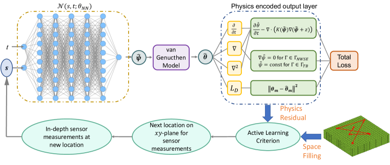
Fig. 1 illustrates our proposed Physics-constrained Deep Active Learning (P-DAL) framework. This framework engages a physics-constrained neural network (P-DL) [11, 22] as a cornerstone to predict the spatial and temporal variations in soil moisture with in situ sensor observations of soil moisture content. Building on the P-DL model, we develop an innovative active learning scheme to identify the most informative locations for placing subsequent soil moisture sensors, thereby enhancing soil moisture prediction of the entire land produced. This active learning strategy employs a combination of physics-informed residual-based sampling and a space-filling design across the land, which will be elaborated in Section III-C.

The characterization of soil moisture majorly depends on the accurate modeling of $\psi(\bm{s},t)$ and $\theta(\bm{s},t)$. We achieve this by using a fully connected feedforward deep neural network (DNN) to approximate the nonlinear relationships between the input spatiotemporal instances $(\bm{s},t)$ and the distribution of the pressure head $\psi$. The DNN output, denoted as $\hat{\psi}$, is anticipated to fulfill two primary conditions: firstly, it should align with the sensor measurements of volumetric moisture content $\theta_{m}$, as depicted by the WRC function in Eq. 4; and secondly, it must adhere to the fundamental physical reality, i.e., RE. Specifically, we model the spatiotemporal pressure head distribution as:

$$[\bm{s},t]\xrightarrow{\mathcal{N}\left(s,t;\Theta_{NN}\right)}\hat{\psi}(\bm{s},t)$$

where $\mathcal{N}\left(s,t;\Theta_{NN}\right)$ is the DNN and $\Theta_{NN}$ denotes the DNN parameters. The DNN contains an input layer encompassing space-time instances $[\bm{s},t]$, several hidden layers to approximate functional relationships between the input and output, and one output layer to estimate $\hat{\psi}(s,t,\Theta_{NN})$. The RE is further embedded into the DNN, together with in situ sensor observations, to form a new loss function defined as:

$$\mathcal{L}(\Theta_{NN})=\mathcal{L}_{D}+\mathcal{L}_{Phy}$$

(7)

The total loss $\mathcal{L}(\Theta_{NN})$ consists of the following two components:

1) Data-driven loss $\mathcal{L}_{D}$: The soil moisture content is measured at multiple locations on the horizontal plane of the field (the $xy$-plane), as well as at differing depths (the $z$ direction) for each selected 2D location. Every sensor captures a time series of soil moisture signals represented by $\theta_{m}(\bm{s},t)$. The DNN is trained to produce predictions, $\hat{\psi}$, that align closely with the actual soil moisture sensor readings, i.e., $\theta_{m}(\bm{s},t)$. Recall that the predicted pressure head $\hat{\psi}$ is related to $\theta$ through the WRC function (i.e., Eq. (4)). Hence, the data-driven loss $\mathcal{L}_{D}$, enforcing agreement between the sensor observations and estimated pressure head $\hat{\psi}_{m}$ values at the placement locations, is formulated as:

$$\mathcal{L}_{D}=\frac{1}{N_{m}}\sum_{i=1}^{N_{m}}(\theta_{m}(\bm{s}_{i},t_{i})-\theta(\hat{\psi}_{m}(\bm{s}_{i},t_{i})))^{2}$$

(8)

where ${N_{m}}$ is the total number of spatiotemporal measurements.

(2) Physcis-based loss $\mathcal{L}_{Phy}$: To improve the predictive accuracy and robustness of the DNN model, we introduce a physics-based constraint at the spatiotemporal collocation points $[\bm{s}_{i},t_{i}],i=1,...,N_{c}$, where $N_{c}$ is the total number of collocation points. These points are randomly selected from the spatiotemporal domain in the target land to encode the physics knowledge for reinforcing the prediction’s adherence to the RE, i.e., Eq. (3). Specifically, the RE-based residual is defined as:

$\displaystyle r(s,t,\Theta_{NN}):=\frac{\partial\theta(\hat{\psi})}{\partial t}-\nabla\cdot(K(\hat{\psi})\nabla(\hat{\psi}+z))$

(9)

The first and second-order partial derivatives of $\psi$ can be efficiently calculated through automatic differentiation, a technique developed for backpropagation in deep learning [38]. The physics-based constraint is enforced by optimizing $r_{\psi}(\bm{s},t;\Theta_{NN})$ towards zero. Consequently, the RE-based loss is defined as:

$$\mathcal{L}_{RE}=\frac{1}{N_{f}}\sum_{i=1}^{N_{f}}\|r(s_{i},t_{i};\Theta_{NN})\|^{2}$$

(10)

where $N_{f}$ is the total number of selected collocation points to enforce the RE.

Similarly, the boundary conditions are incorporated in the model in terms of the boundary-related residuals. The boundary conditions in Eq. (LABEL:Eq:boundary1-LABEL:Eq:boundary2) can be concisely represented as $\mathcal{B}(\psi,\bm{s},t)=0$ on $\Gamma$ which stands for the boundaries. To ensure that the prediction $\hat{\psi}$ is consistent with the boundary conditions, we define the boundary condition-based loss as:

$$\mathcal{L}_{\mathcal{B}}=\frac{1}{|\Gamma|}\sum_{\bm{s}\in\Gamma}\|\mathcal{B}(\hat{\psi},\bm{s},t)\|^{2}_{2}$$

(11)

Then, $\mathcal{L}_{\mathcal{B}}$ joins the RE-based loss to create the physics-based loss: $\mathcal{L}_{Phy}=\mathcal{L}_{RE}+\mathcal{L}_{\mathcal{B}}$, which is then combined with the data-driven loss (Eq. (8)) to formulate the overall loss function in Eq. (7). This loss setting in DNN allows for a comprehensive consideration of both sensor readings and the fundamental physics governing the water flow dynamics in soil, which will enable the reliable modeling of the spatiotemporal soil moisture dynamics.

Even though the involvement of physics regularization can alleviate the model reliance on the training data, the quality and volume of training data can still significantly impact the model performance [39, 22]. The cost associated with deploying sensors becomes a significant factor for soil moisture monitoring in a large field. Optimal sensor placement is urgently needed to enable the use of a limited number of in situ sensors while still maintaining high-quality predictive modeling of soil moisture dynamics. Note that the high-resolution 3D mapping of soil moisture is predicted in light of the recorded time-series data from sensor placement locations. By strategically positioning sensors, we can capture the spatial variability in soil moisture more accurately, which is vital for quantitatively monitoring soil moisture distribution and managing crop irrigation. Here, we introduce a novel active learning approach that fuses residual-based sampling with a space-filling strategy. The goal is to collect the most essential time series data for training the P-DL model so that the model outcome remains robust even with a limited number of sensors.

(1) Residual-based sampling: Traditional methods for seeking the sensor location in soil moisture systems mostly depend on exploring the statistical insights of the model output or graphical interrelationships [30, 31, 32]. These methods ignore the underlying physics truth that governs the soil moisture dynamics. Additionally, due to their specially designed model infrastructure for estimating soil moisture, these sensor placement algorithms may not be readily applied in a deep learning framework. Inspired by the work of Katharopoulos and Fleuret [40], which demonstrate that the selection of training samples based on loss magnitude can expedite the convergence of neural network optimization, we propose an innovative residual-based sampling strategy for robust prediction of soil moisture using P-DL.

The proposed residual-based sampling scheme aims to find the most informative location on a horizontal land (i.e., $xy$-plane) by identifying a spatial location with the largest residual value on the 2D plane. Similar to Eq. (9), the residual for every spatial node in the soil geometry and temporal instance can be calculated by:

	$\displaystyle r(\bm{s}_{i},t_{j},\Theta_{NN}):=\frac{\partial\theta}{\partial t}-\nabla\cdot\left(K(\hat{\psi}(\bm{s}_{i},t_{j}))\nabla(\hat{\psi}(\bm{s}_{i},t_{j})+z)\right)$		(12)
	$\displaystyle\text{for }i=1,\dots,N\text{ and }j=1,\dots,T.$

where $\bm{s}_{i}\in\mathbb{R}^{3}$, $N$ is the total number of discretized spatial nodes and $T$ is the total number of temporal instances. Let $N_{L},N_{W},N_{D}$ be the number of the discretized spatial nodes for the soil geometry’s length, width, and depth, respectively. This leads to $N=N_{L}N_{W}N_{D}$. We denote $r_{\bm{\kappa}}$ as the cumulative residual over different depths and time instances for a given location on the $xy$-plane.

$\displaystyle r_{\bm{\kappa}}(x_{l},y_{w},\Theta_{NN})=\sum_{j=1}^{T}\sum_{d=1}^{N_{D}}\|r(x_{l},y_{w},z_{d},t_{j},\Theta_{NN})\|^{2}$

(13)

where $l=1,...,L$ and $w=1,...,W$. We use min-max normalization to rescales $r_{\bm{\kappa}}$ to the range $[0,1]$:

$$r^{\prime}_{\bm{\kappa}}=\frac{r_{\bm{\kappa}}-r_{\bm{\kappa}\min}}{r_{\bm{\kappa}\max}-r_{\bm{\kappa}\min}}$$

(14)

where $r^{\prime}_{\bm{\kappa}}$ represents the normalized values for the residuals in $xy$-plane. $r_{\bm{\kappa}\min}$ and $r_{\bm{\kappa}\min}$ stand for the minimum and maximum value of $r_{\bm{\kappa}}$, respectively. The location index exhibiting the largest $r_{\bm{\kappa}}^{\prime}$ value indicates that the prediction at this specific 2D location deviates most significantly from the established physics-based model, the Richards equation.

The residual-based active sampling may enable faster convergence for neural network training. Lu et al. [39] first proposed a residual-based adaptive refinement to improve the distribution of residual points during the training process. Based on this, Yu et al. [41] and Wu et al . [42] propose to adaptively add training data where the residuals are large to improve the prediction. However, in cases where residuals are non-uniform or have significant variations across the 2D domain, residual-based sampling alone might struggle to adequately identify proper sensor locations that carry global information about soil moisture dynamics.

(2) Space-filling design: To enhance global soil moisture prediction with P-DL, we propose to further incorporate the maximin-distance design, a space-filling approach for optimizing computer experiments, into our active learning framework. Let $\bm{\kappa}=[x,y]$ denote the spatial location in $xy$-plane. In the conventional sequential learning process that relies on a purely space-filling design, the subsequent query point $\bm{\kappa}_{n+1}$ is determined by:

$\displaystyle\bm{\kappa}_{n+1}=\arg\max_{\bm{\kappa}}\min_{i\in\{1,2,...,n\}}\mathrm{dist}(\bm{\kappa},\bm{\kappa}_{i})$

(15)

This approach generates the subsequent point $\bm{\kappa}_{n+1}$ by ensuring it has the maximum possible minimum distance from the already observed locations $\bm{\kappa}_{i}$’s, $i\in\{1,\dots,n\}$. The Euclidean distance function $dist(\cdot)$ is employed in Eq. (15) to account for the spatial interplays in a 2D field. This will then be combined with the residual-based sampling scheme to form a new active learning criterion.

(3) Active learning criterion: A good active learning (AL) criterion for a physical system shall account for both the deviation degree from the fundamental laws and the distribution level of chosen observation locations. To meet this objective, we design a new AL criterion that integrates the residual magnitude with the max-min design as:

$\displaystyle\bm{\kappa}_{n+1}=\operatorname{argmax}_{\bm{\kappa}}\left\{r^{\prime}_{\bm{\kappa}}(\bm{\kappa})+\lambda\cdot\frac{\min\limits_{i\in\{1,\cdots,n\}}\mathrm{dist}\left(\bm{\kappa}-\bm{\kappa}_{i}\right)}{\max\limits_{\bm{\kappa}}\min\limits_{i\in\{1,\cdots,n\}}\mathrm{dist}\left(\bm{\kappa}-\bm{\kappa}_{i}\right)}\right\}$

(16)

where $\min_{i\in\{1,\cdots,n\}}\mathrm{dist}\left(\bm{\kappa}-\bm{\kappa}_{i}\right)$ is the shortest distance from the unobserved location $\bm{\kappa}$ to any of the measured location $\bm{\kappa}_{i}$’s, $i\in\{1,\dots,n\}$ on the horizontal plane. The greatest possible value of these minimum distances is expressed as $\max_{\bm{\kappa}}\min_{i\in\{1,\cdots,n\}}\mathrm{dist}\left(\bm{\kappa}-\bm{\kappa}_{i}\right)$, which serves to normalize the space-filling criterion. Parameter $\lambda>0$ is introduced to balance between the influences of the selection based on residuals and space-filling design. Its value is empirically set as 1 in later numerical experiments. The proposed AL criterion in Eq. (16) is designed to find the potential sensor locations that carry the most comprehensive information about the entire soil moisture dynamics. The 2D locations indicated by the AL criterion highlight areas with low physical fidelity while simultaneously considering the global perspective, thereby enhancing the predictive power of P-DL.

In the active learning process, one spatial location on the $xy$-plane is initially randomly chosen. Note that, for each selected 2D location, 5 sensors are installed at different depths. Those initial sensor readings will be used to train the P-DL model. After the training is complete, we further apply the AL criterion to determine the next sampling point on the $xy$-plane. We measure the soil moisture at various depths at the new location. The resulting time series data is incorporated into the training dataset to re-train the P-DL model. This active selection iterates itself until the sensor budget is exhausted.

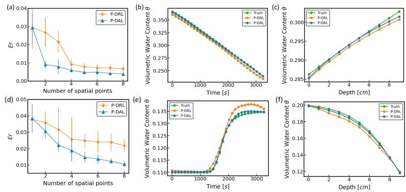
Fig. 3(a) illustrates the performance of the P-DL model trained using sensor data gathered via the proposed active learning with uniform random sampling. Specifically, one location on the horizontal plane is selected for each sampling round. For each sampling round, one single location on the horizontal plane is chosen, and 5 soil moisture sensors are uniformly distributed along the vertical axis. To mitigate the variability inherent in network training, the P-DL model is trained 10 times for each sampling round. The mean of the resulting 10 $Er$ values is calculated to ensure consistency in our results. Furthermore, to depict the variability of the $Er$ values, we have included error bars, calculated from the standard deviation, presented in Fig. 3(a). In Fig. 3(b-c), we select the prediction of soil moisture dynamics that exhibits $Er$ closest to the calculated mean. This allows us to showcase a representative model performance that aligns closely with the average prediction accuracy.

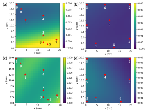
Figs. 2(a) and (b) show the absolute error in soil moisture between the predictions of P-DRL and P-DAL with the noise-added benchmark, respectively, in the $xy$-plane at an arbitrary depth and time. The figures also illustrate the placement sequence and locations of soil moisture sensors on the $xy$-plane. A brighter color indicates a larger discrepancy from the ground truth. Thus, from Figs. 2(a) and (b), we see that, unlike uniform random selection, our active learning approach, informed by physics-based residuals, selects more spatially distributed locations. Thus, this strategy improves the global accuracy of soil moisture dynamic estimation, as evidenced by smaller discrepancies (darker color) in the mapping.

As illustrated in Fig. 3(a), when the number of spatial points increases, $Er$ reduces. This is because more information on the soil moisture is incorporated into the P-DL model. However, the $Er$ provided by our P-DAL model shows a more rapid decline as opposed to the $Er$ estimated by P-DRL. The $Er$ values given by P-DAL and P-DRL start to separate after the first sampling round. When the number of the selected spatial points on the horizontal plane reaches 8, which means that the sensor budget of 40 is all used, the $Er$ is reduced to $3.89\times 10^{-3}$ by P-DAL, which is 42.4% less than the $Er$ of P-DRL ($6.75\times 10^{-3}$). This suggests that the proposed P-DAL method can robustly model the soil moisture dynamics, (i.e., volumetric water content), in the crop field with $N=4000$ spatial nodes at a relative error of $3.89\times 10^{-3}$ with just 40 sensing locations (8 selected locations on the horizontal plane and 5 sensors installed at different depths for each horizontal location).

Fig. 3(b) presents the evolution of the soil moisture content $\hat{\theta}$ overtime at a specific location, as estimated by the P-DL model. Fig. 3(c) demonstrates the variation of $\hat{\theta}$ along the $z$-axis at a specific 2D location on the horizontal plane at an arbitrary time point. The estimations are based on the data collected from 40 sensors, with the locations of these sensors determined by employing P-DAL or P-DRL. The predictions are benchmarked by the ground truth dynamic evolution (green curve). Both approaches produce good predictions thanks to the physics-based constraint embedded in the P-DL model. However, upon closer examination of Fig. 3(b-c), it becomes evident that P-DAL shows better alignment with the ground truth compared to the P-DRL model. This demonstrates the superior performance of our P-DAL strategy in strategically selecting sensor locations that reduce the variability the most.

Fig. 3(d) illustrates the forecasting ability of the P-DL model when trained with datasets obtained via active learning (i.e., P-DAL) and uniform random selection (i.e., P-DRL). The P-DAL method demonstrates lower $Er$ overall than those produced by the P-DRL. The deviation starts to show up after the first round of sensor placement selection. When the total number of sensors ($N=40$) are all deployed, the $Er$ is reduced to 0.0105 for P-DAL in comparison with the $Er$ of 0.0218 by P-DRL, a 51.8% difference. Figs. 2(b) and (c) show P-DRL and P-DAL predicted mappings, respectively, for the infiltration. Similar to the evaporation case, the active learning strategy optimizes sensor placement for enhanced soil moisture estimation with minimal absolute discrepancy from the ground truth.

Note that the infiltration case presents a more complex soil moisture dynamic pattern compared to evaporation, where the moisture curves tend to be more gradual. This is due to infiltration’s heightened sensitivity to external variables, such as rainfall intensity. These factors can cause swift changes in soil moisture levels and create steep moisture gradients as water percolates through the soil. This will increase the difficulty of P-DL model prediction and lead to the estimation error of infiltration higher than the evaporation case.

Fig. 3(e) illustrates the temporal evolution of estimated soil moisture, $\hat{\theta}$, at a designated location, as predicted by the P-DL model. Meanwhile, Fig. 3(f) highlights the variation in $\hat{\theta}$ along the vertical direction at a particular 2D point on the horizontal plane, captured at a chosen time point. These estimations are obtained from the output of the DNNs trained by data gathered via the active learning scheme as well as the conventional uniform random sampling method. The prediction accuracy is compared against the actual dynamic development (green curve). Similar to the evaporation scenario, both sampling strategies show an accurate overall trend. However, a detailed review of Figs. 3(e-f) reveals that the P-DAL-generated curves exhibit closer conformity to the empirical data compared to the P-DRL outcomes. This difference reconfirms the effectiveness of our P-DAL approach in identifying optimal sensor placements that would improve the precision of spatiotemporal soil moisture dynamics modeling.

References

- [1] D. A. Robinson, C. S. Campbell, J. W. Hopmans, B. K. Hornbuckle, S. B. Jones, R. Knight, F. Ogden, J. Selker, and O. Wendroth, “Soil moisture measurement for ecological and hydrological watershed-scale observatories: A review,” Vadose Zone Journal, vol. 7, no. 1, pp. 358–389, 2008.
- [2] E. Babaeian, M. Sadeghi, S. B. Jones, C. Montzka, H. Vereecken, and M. Tuller, “Ground, proximal, and satellite remote sensing of soil moisture,” Reviews of Geophysics, vol. 57, no. 2, pp. 530–616, 2019.
- [3] F. L. Ogden, M. B. Allen, W. Lai, J. Zhu, M. Seo, C. C. Douglas, and C. A. Talbot, “The soil moisture velocity equation,” Journal of Advances in Modeling Earth Systems, vol. 9, no. 2, pp. 1473–1487, 2017.
- [4] J. Simunek, M. T. Van Genuchten, and M. Sejna, “The hydrus software package for simulating two-and three-dimensional movement of water, heat, and multiple solutes in variably-saturated media,” Technical manual, version, vol. 1, p. 241, 2006.
- [5] Z. Song and Jiang Z*, “A data-driven modeling approach for water flow dynamics in soil,” Computer Aided Chemical Engineering, vol. 52, pp. 819–824, 2023.
- [6] Z. Song and Z. Jiang, “A data-facilitated numerical method for richards equation to model water flow dynamics in soil,” arXiv preprint arXiv:2310.02806, 2023.
- [7] L. Pasolli, C. Notarnicola, and L. Bruzzone, “Estimating soil moisture with the support vector regression technique,” IEEE Geoscience and remote sensing letters, vol. 8, no. 6, pp. 1080–1084, 2011.
- [8] Y. Liu, Y. Yang, W. Jing, and X. Yue, “Comparison of different machine learning approaches for monthly satellite-based soil moisture downscaling over northeast china,” Remote Sensing, vol. 10, no. 1, p. 31, 2017.
- [9] Y. Liu, W. Jing, Q. Wang, and X. Xia, “Generating high-resolution daily soil moisture by using spatial downscaling techniques: A comparison of six machine learning algorithms,” Advances in Water Resources, vol. 141, p. 103601, 2020.
- [10] I. Ali, F. Greifeneder, J. Stamenkovic, M. Neumann, and C. Notarnicola, “Review of machine learning approaches for biomass and soil moisture retrievals from remote sensing data,” Remote Sensing, vol. 7, no. 12, pp. 16 398–16 421, 2015.
- [11] J. Xie and B. Yao, “Physics-constrained deep learning for robust inverse ecg modeling,” IEEE Transactions on Automation Science and Engineering, 2022.
- [12] D. Shen, G. Wu, and H.-I. Suk, “Deep learning in medical image analysis,” Annual review of biomedical engineering, vol. 19, p. 221, 2017.
- [13] Y. Cai, W. Zheng, X. Zhang, L. Zhangzhong, and X. Xue, “Research on soil moisture prediction model based on deep learning,” PloS one, vol. 14, no. 4, p. e0214508, 2019.
- [14] Y. LeCun, Y. Bengio, and G. Hinton, “Deep learning,” nature, vol. 521, no. 7553, pp. 436–444, 2015.
- [15] J. Yu, X. Zhang, L. Xu, J. Dong, and L. Zhangzhong, “A hybrid cnn-gru model for predicting soil moisture in maize root zone,” Agricultural Water Management, vol. 245, p. 106649, 2021.
- [16] L. Li, Y. Dai, W. Shangguan, Z. Wei, N. Wei, and Q. Li, “Causality-structured deep learning for soil moisture predictions,” Journal of Hydrometeorology, vol. 23, no. 8, pp. 1315–1331, 2022.
- [17] M. Raissi, P. Perdikaris, and G. E. Karniadakis, “Physics-informed neural networks: A deep learning framework for solving forward and inverse problems involving nonlinear partial differential equations,” Journal of Computational physics, vol. 378, pp. 686–707, 2019.
- [18] M. Raissi, A. Yazdani, and G. E. Karniadakis, “Hidden fluid mechanics: Learning velocity and pressure fields from flow visualizations,” Science, vol. 367, no. 6481, pp. 1026–1030, 2020.
- [19] C. Rao, H. Sun, and Y. Liu, “Physics-informed deep learning for computational elastodynamics without labeled data,” Journal of Engineering Mechanics, vol. 147, no. 8, p. 04021043, 2021.
- [20] R. Zhang, Y. Liu, and H. Sun, “Physics-informed multi-lstm networks for metamodeling of nonlinear structures,” Computer Methods in Applied Mechanics and Engineering, vol. 369, p. 113226, 2020.
- [21] S. Cai, Z. Wang, S. Wang, P. Perdikaris, and G. E. Karniadakis, “Physics-Informed Neural Networks for Heat Transfer Problems,” Journal of Heat Transfer, vol. 143, no. 6, p. 060801, Apr. 2021. [Online]. Available: https://doi.org/10.1115/1.4050542
- [22] J. Xie and B. Yao, “Physics-constrained deep active learning for spatiotemporal modeling of cardiac electrodynamics,” Computers in Biology and Medicine, vol. 146, p. 105586, 2022.
- [23] L. A. Richards, “Capillary conduction of liquids through porous mediums,” Physics, vol. 1, no. 5, pp. 318–333, 1931.
- [24] A. M. Tartakovsky, C. O. Marrero, P. Perdikaris, G. D. Tartakovsky, and D. Barajas-Solano, “Learning parameters and constitutive relationships with physics informed deep neural networks,” arXiv preprint arXiv:1808.03398, 2018.
- [25] T. Bandai and T. A. Ghezzehei, “Physics-informed neural networks with monotonicity constraints for richardson-richards equation: Estimation of constitutive relationships and soil water flux density from volumetric water content measurements,” Water Resources Research, vol. 57, no. 2, p. e2020WR027642, 2021.
- [26] I. Depina, S. Jain, S. Mar Valsson, and H. Gotovac, “Application of physics-informed neural networks to inverse problems in unsaturated groundwater flow,” Georisk: Assessment and Management of Risk for Engineered Systems and Geohazards, vol. 16, no. 1, pp. 21–36, 2022.
- [27] P. Haruzi and Z. Moreno, “Modeling water flow and solute transport in unsaturated soils using physics-informed neural networks trained with geoelectrical data,” Water Resources Research, vol. 59, no. 6, p. e2023WR034538, 2023.
- [28] G. Gullickson, “Soil-moisture sensors,” https://www.agriculture.com/machinery/precision-agriculture/soilmoisture-senss_234-ar42409, March 2014, accessed February 2024.
- [29] L. Zotarelli, M. Dukes, and M. Paranhos, “Minimum number of soil moisture sensors for monitoring and irrigation purposes,” https://edis.ifas.ufl.edu/pdf/HS/HS1222/HS1222-11819701.pdf, September 2019, accessed February 2024.
- [30] X. Wu, M. Liu, and Y. Wu, “In-situ soil moisture sensing: Optimal sensor placement and field estimation,” ACM Transactions on Sensor Networks (TOSN), vol. 8, no. 4, pp. 1–30, 2012.
- [31] M. Dursun and S. Özden, “Optimization of soil moisture sensor placement for a pv-powered drip irrigation system using a genetic algorithm and artificial neural network,” Electrical Engineering, vol. 99, pp. 407–419, 2017.
- [32] S. R. Sahoo, X. Yin, and J. Liu, “Optimal sensor placement for agro-hydrological systems,” AIChE Journal, vol. 65, no. 12, p. e16795, 2019.
- [33] E. Buckingham, Studies on the movement of soil moisture. United States Department of Agriculture, United States Bureau of Soils, 1907.
- [34] S. Assouline, “Modeling the relationship between soil bulk density and the hydraulic conductivity function,” Vadose Zone Journal, vol. 5, no. 2, pp. 697–705, 2006.
- [35] R. Brooks and A. Corey, “Hydraulic properties of porous media. hydrology paper no. 3,” Civil Engineering Department, Colorado State University, Fort Collins, CO, 1964.
- [36] M. T. Van Genuchten, “A closed-form equation for predicting the hydraulic conductivity of unsaturated soils,” Soil science society of America journal, vol. 44, no. 5, pp. 892–898, 1980.
- [37] M. A. Celia and P. Binning, “A mass conservative numerical solution for two-phase flow in porous media with application to unsaturated flow,” Water Resources Research, vol. 28, no. 10, pp. 2819–2828, 1992.
- [38] A. Paszke, S. Gross, S. Chintala, G. Chanan, E. Yang, Z. DeVito, Z. Lin, A. Desmaison, L. Antiga, and A. Lerer, “Automatic differentiation in pytorch,” 2017.
- [39] L. Lu, X. Meng, Z. Mao, and G. E. Karniadakis, “Deepxde: A deep learning library for solving differential equations,” SIAM review, vol. 63, no. 1, pp. 208–228, 2021.
- [40] A. Katharopoulos and F. Fleuret, “Biased importance sampling for deep neural network training,” arXiv preprint arXiv:1706.00043, 2017.
- [41] J. Yu, L. Lu, X. Meng, and G. E. Karniadakis, “Gradient-enhanced physics-informed neural networks for forward and inverse pde problems,” Computer Methods in Applied Mechanics and Engineering, vol. 393, p. 114823, 2022.
- [42] C. Wu, M. Zhu, Q. Tan, Y. Kartha, and L. Lu, “A comprehensive study of non-adaptive and residual-based adaptive sampling for physics-informed neural networks,” Computer Methods in Applied Mechanics and Engineering, vol. 403, p. 115671, 2023.
- [43] J. Varela, “Implementation of an mpfa/mpsa-fv solver for the unsaturated flow in deformable porous media,” Master’s thesis, The University of Bergen, 2018.