Physics-informed GANs for coastal flood visualization
Abstract
As climate change increases the intensity of natural disasters, society needs better tools for adaptation. Floods, for example, are the most frequent natural disaster, but during hurricanes the area is largely covered by clouds and emergency managers must rely on nonintuitive flood visualizations for mission planning. To assist these emergency managers, we have created a deep learning pipeline that generates visual satellite images of current and future coastal flooding. We advanced a state-of-the-art GAN called pix2pixHD, such that it produces imagery that is physically-consistent with the output of an expert-validated storm surge model (NOAA SLOSH). By evaluating the imagery relative to physics-based flood maps, we find that our proposed framework outperforms baseline models in both physical-consistency and photorealism. While this work focused on the visualization of coastal floods, we envision the creation of a global visualization of how climate change will shape our earth101010Code and data will be made available at github.com/repo; an interactive demo at trillium.tech/eie..
1 Introduction
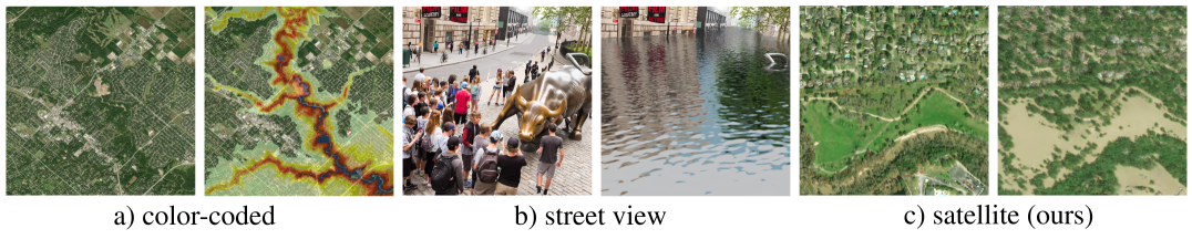
As our climate changes, natural disasters become more intense [2]. Floods are the most frequent weather-related disaster [3] and already cost the U.S. per year; this damage will only grow over the next several decades [4, 2]. Today, emergency managers and local decision-makers rely on visualizations to understand and communicate flood risks (e.g., building damage) [5]. Shortly after a coastal flood, however, clouds cover the affected area and before a coastal flood no RGB satellite imagery exists to plan flood response or resilience strategies. Existing visualizations are limited to informative overviews (e.g., color-coded maps [5, 1, 6]) or intuitive (i.e., photorealistic) street-view imagery [7, 8]. Expert interviews, however, suggest that color-coded maps (displayed in Fig.˜2a) are non-intuitive and can complicate communication among decision makers [9]. Street-view imagery (displayed in Fig.˜2b), on the other hand, offers intuitive understanding of flood damage, but remains too local for city-wide planning [9]. To assist with both climate resilience and disaster response planning, we propose the first deep learning pipeline that generates satellite imagery of coastal floods, creating visualizations that are both intuitive and informative.
Recent advances in generative adversarial networks (GANs) generated photorealistic imagery of faces [12, 13], animals [14, 15], or even satellite [16, 17], and street-level flood imagery [7]. Disaster planners and responders, however, need imagery that is not only photorealistic, but also physically-consistent. In our implementation, we consider both GANs and variational autoencoders (VAEs), where GANs generate more photorealistic imagery ([18, 19], Fig.˜3) and VAEs capture system uncertainties more accurately [20, 21]. Because our use case requires photorealism to provide intuition, we extend a state-of-the-art, high-resolution GAN, pix2pixHD [13], to take in physical constraints and produce imagery that is both photorealistic and physically-consistent. We leave ensemble predictions to account for system uncertainties for future work.
There are multiple approaches to generating physically-consistent imagery with GANs, where we define physically-consistent to assess: Does the generated imagery depict the same flood extent as the storm surge model? One approach is conditioning the GAN on the outputs of physics-based models [22]; another approach is using a physics-based loss during evaluation [23]; and yet another is embedding the neural network in a differential equation [24] (e.g., as parameters, dynamics [25], residual [26], differential operator [27, 28], or solution [29]). Our work focuses on the first two methods, leveraging years of scientific domain knowledge by incorporating a physics-based storm surge model in the image generation and evaluation pipeline.
This work makes three contributions: 1) the first physically-consistent visualization of coastal flood model outputs as high-resolution, photorealistic satellite imagery; 2) a novel metric, the Flood Visualization Plausibility Score (FVPS), to evaluate the photorealism and physical-consistency of generated imagery; and 3) an extensible framework to generate physically-consistent visualizations of climate extremes.
2 Approach
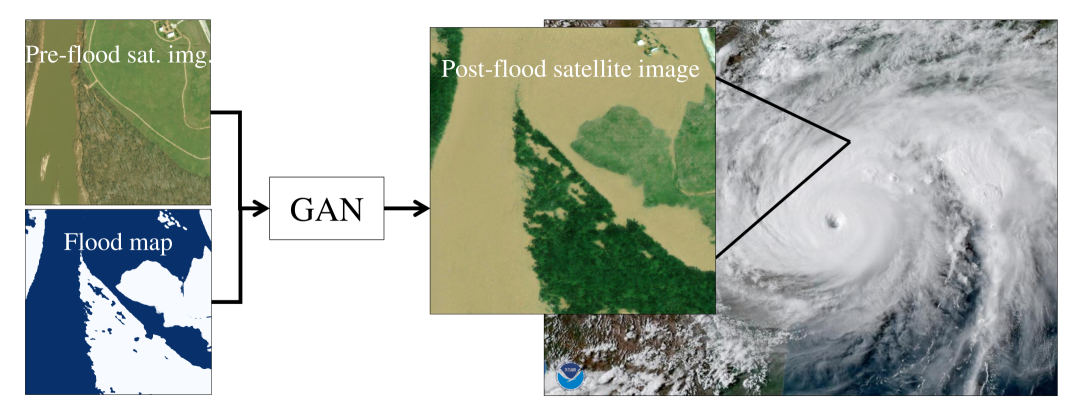
The proposed pipeline uses a generative vision model to generate post-flooding images from pre-flooding images and a flood extent map, as shown in Fig.˜1.
Data Overview. Obtaining post-flood images that display standing water is challenging due to cloud-cover, time of standing flood, satellite revisit rate, and cost of high-resolution imagery. This work leverages the xBD dataset [11], a collection of pre- and post-disaster images from events like Hurricane Harvey or Florence, from which we obtained pre- and post-flooding image pairs with the following characteristics: , RGB, (post-processing details in Section˜5.2). We also downloaded flood hazard maps (at ), which are outputs of NOAA’s widely used storm surge model, SLOSH, that models the dynamics of hurricane winds pushing water on land (Section˜5.2). We then aligned the flood hazard map with the flood images and reduced it into a binary flood extent mask (flooded vs. non-flooded).
Model architecture. The central model of our pipeline is a generative vision model that learns the physically-conditioned image-to-image transformation from pre-flood image to post-flood image. We leveraged the existing implementation of the GAN pix2pixHD [13] and extended the input dimensions to to incorporate the flood extent map. Note that the pipeline is modular, such that it can be repurposed for visualizing other climate impacts.
The Evaluation Metric Flood Visualization Plausibility Score (FVPS). Evaluating imagery generated by a GAN is difficult [30, 31]. Most evaluation metrics measure photorealism or sample diversity [31], but not physical consistency [32] (see, e.g., SSIM [33], MMD [34], IS [35], MS [36] , FID [37, 38], or LPIPS [39]).
To evaluate physical consistency, as defined in Section˜1, we propose using the intersection over union (IoU) between water in the generated imagery and water in the flood extent map. This method relies on flood masks, but because there are no publicly available flood segmentation models for RGB imagery, we trained our own model on hand-labeled flooding images (Section˜5.2). This segmentation model produced flood masks of the generated and ground-truth flood image which allowed us to measure the overlap of water in between both. When the flood masks overlap perfectly, the IoU is 1; when they are completely disjoint, the IoU is 0.
To evaluate photorealism, we used the state-of-the-art perceptual similarity metric Learned Perceptual Image Patch Similarity (LPIPS) [39]. LPIPS computes the feature vectors (of an ImageNet-pretrained deep CNN, AlexNet) of the generated and ground-truth tile and returns the mean-squared error between the feature vectors (best LPIPS is , worst is ).
Because the joint optimization over two metrics poses a challenging hyperparameter optimization problem, we propose to combine the evaluation of physical consistency (IoU) and photorealism (LPIPS) in a new metric (FVPS), called Flood Visualization Plausibility Score (FVPS). The FVPS is the harmonic mean over the submetrics, IoU and , that are both -bounded. Due to the properties of the harmonic mean, the FVPS is if any of the submetrics is ; the best FVPS is .
| (1) |
3 Experimental Results
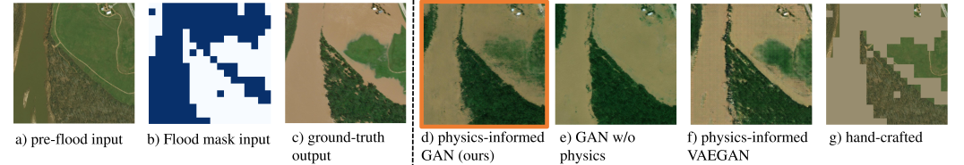
In terms of both physical-consistency and photorealism, our physics-informed GAN outperforms an unconditioned GAN that does not use physics, as well as a handcrafted baseline model (Fig.˜3).
A GAN without physics information generates photorealistic but non physically-consistent imagery. The inaccurately modeled flood extent in Fig.˜3e illustrates the physical-inconsistency and a low IoU of in Table˜1 over the test set further confirms it (see Section˜5.2 for test set details). Despite the photorealism (), the physical-inconsistency renders the model non-trustworthy for critical decision making, as confirmed by the low FVPS of . The model is the default pix2pixHD [13], which only uses the pre-flood image and no flood mask as input.
A handcrafted baseline model generates physically-consistent but not photorealistic imagery. Similar to common flood visualization tools [6], the handcrafted model overlays the flood mask input as a hand-picked flood brown (#998d6f) onto the pre-flood image, as shown in Fig.˜3g. Because typical storm surge models output flood masks at low resolution ( [1]), the handcrafted baseline generates pixelated, non-photorealistic imagery. Combining the high IoU of and the poor LPIPS of , yields a low FVPS score of , highlighting the difference to the physics-informed GAN in a single metric.
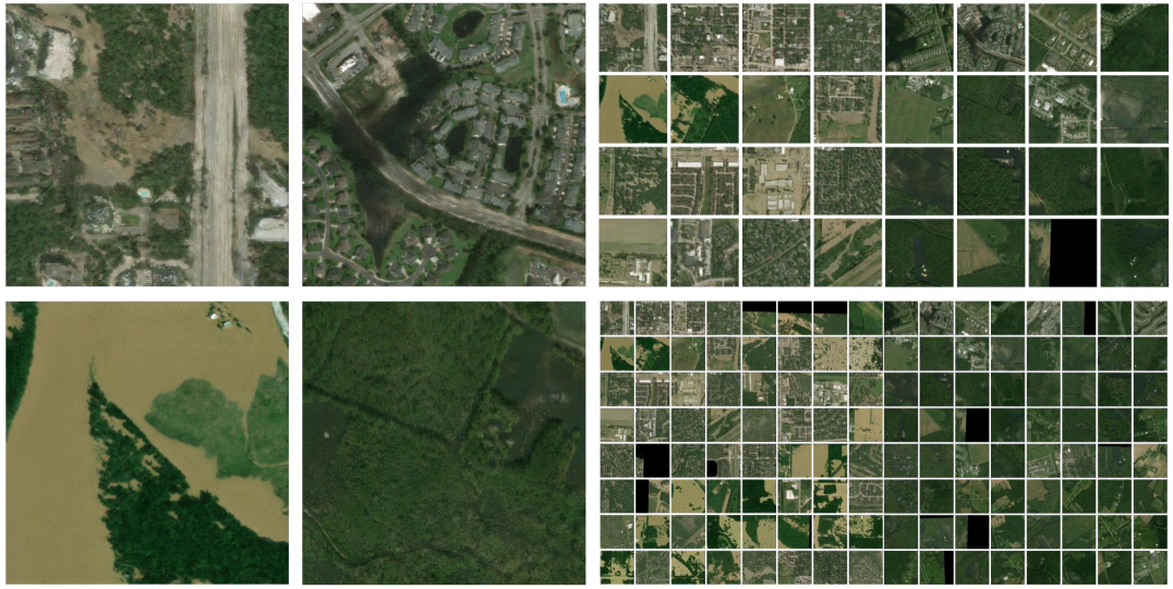
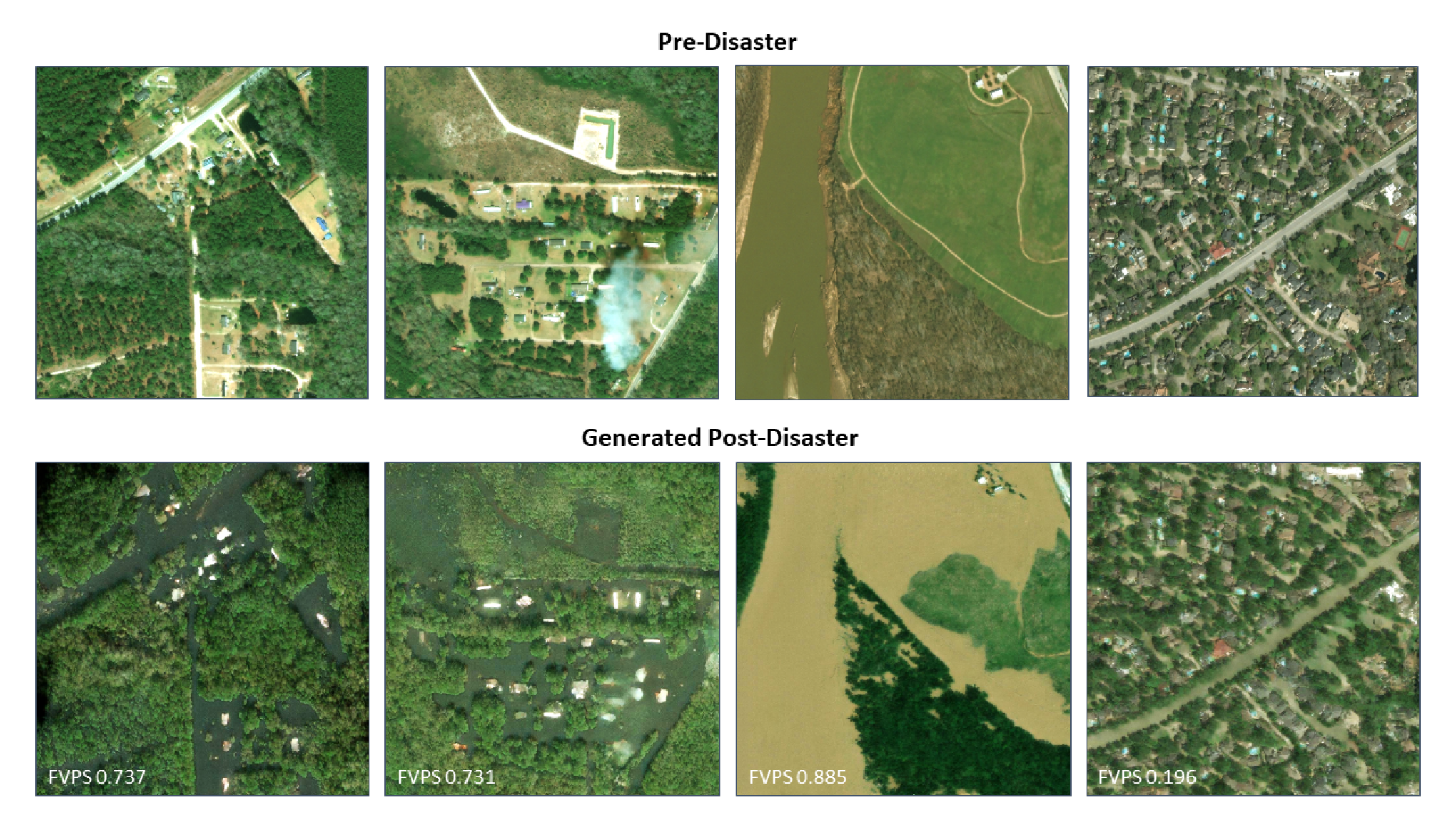
The proposed physics-informed GAN generates physically-consistent and photorealistic imagery. To create the physics-informed GAN, we trained pix2pixHD [13] from scratch on our dataset ( on Google Cloud GPUs). This model successfully learned how to convert a pre-flood image and a flood mask into a photorealistic post-flood image, as shown in Fig.˜5. The model outperformed all other models in IoU (), LPIPS (), and FVPS () (Table˜1). The learned image transformation “in-paints“ the flood mask in the correct flood colors and displays an average flood height that does not cover structures (e.g., buildings, trees), as shown in randomly sampled test images in Fig.˜4. While our model also outperforms the VAEGAN (BicyleGAN), the latter has the potential to create ensemble forecasts over the unmodeled flood impacts, such as the probability of destroyed buildings.
| LPIPS high res. | LPIPS low res. | IoU high res. | LPIPS low res. | FVPS high res. | FVPS low res. | |
|---|---|---|---|---|---|---|
| GAN w/ phys. (ours) | 0.265 | 0.283 | 0.502 | 0.365 | 0.533 | 0.408 |
| GAN w/o phys. | 0.293 | 0.293 | 0.226 | 0.226 | 0.275 | 0.275 |
| VAEGAN w/ phys. | 0.449 | - | 0.468 | - | 0.437 | - |
| Handcrafted baseline | 0.399 | 0.415 | 0.470 | 0.361 | 0.411 | 0.359 |
4 Discussion and Future Work
Although our pipeline outperformed all baselines in the generation of physically-consistent and photorealistic imagery of coastal floods, there are areas for improvement in future works. For example, our dataset only contained samples and is biased towards vegetation-filled satellite imagery; this data limitation likely contributes to our model rendering human-built structures, such as streets and out-of-distribution skyscrapers in Fig.˜4 top-left, as smeared. In addition, the dataset was generated by Maxar imagery and preliminary results suggest that our model does not generalize well to other data sources such as NAIP imagery [10]. Although we attempted to overcome our data limitations using several state-of-the-art augmentation techniques, this work would benefit from more public sources of high-resolution satellite imagery (experiment details in Section˜5.3). Finally, the computational intensity of training GANs made it difficult to fine-tune models on new data; improved transfer learning techniques could address this challenge. Lastly, satellite imagery is an internationally trusted source for analyses in deforestation, development, or military [40, 41], and with the rise of “deep-fake“ models, more work is needed in the identification of and education around misinformation and ethical AI [42]. Given our pipeline’s results, however, we hope to deploy with NOAA by integrating flood forecasts with aerial imagery along the entire U.S. East Coast.
Vision for the future. We envision a global visualization tool for climate impacts. Our proposed pipeline can generalize in time, space, and type of event. By changing the input data, future work can visualize impacts of other well-modeled, climate-attributed events, including arctic sea ice melt, wildfires, or droughts. Non-binary climate impacts, such as inundation height, or drought strength can be generated by replacing the binary flood mask with continuous model predictions. Opportunities are abundant for further work in visualizing our changing Earth, and given its potential impact for both climate mitigation and adaptation, we encourage the ML community to take up this challenge.
Acknowledgments
This research was conducted at the Frontier Development Lab (FDL), US. The authors gratefully acknowledge support from the MIT Portugal Program, National Aeronautics and Space Administration (NASA), and Google Cloud. Further, we greatly appreciate the time, feedback, direction, and help from Prof. Bistra Dilkina, Ritwik Gupta, Mark Veillette, Capt. John Radovan, Peter Morales, Esther Wolff, Leah Lovgren, Guy Schumann, Freddie Kalaitzis, Richard Strange, James Parr, Sara Jennings, Jodie Hughes, Graham Mackintosh, Michael van Pohle, Gail M. Skofronick-Jackson, Tsengdar Lee, Madhulika Guhathakurta, Julien Cornebise, Maria Molina, Massy Mascaro, Scott Penberthy, Derek Loftis, Sagy Cohen, John Karcz, Jack Kaye, Janot Mendler de Suarez, Campbell Watson, and all other FDL researchers.
Björn Lütjens and Brandon Leshchinskiy’s research has been partially sponsored by the United States Air Force Research Laboratory and the United States Air Force Artificial Intelligence Accelerator and was accomplished under Cooperative Agreement Number FA8750-19-2-1000. The views and conclusions contained in this document are those of the authors and should not be interpreted as representing the official policies, either expressed or implied, of the United States Air Force or the U.S. Government. The U.S. Government is authorized to reproduce and distribute reprints for Government purposes notwithstanding any copyright notation herein.
References
- [1] NOAA National Weather Service National Hurrican Center Storm Surge Prediction Unit, “National Storm Surge Hazard Maps, Texas to Maine, Category 5,” 2020. [Online]. Available: https://noaa.maps.arcgis.com/apps/MapSeries/index.html?appid=d9ed7904dbec441a9c4dd7b277935fad&entry=1
- [2] IPCC, “Global warming of 1.5c. an ipcc special report on the impacts of global warming of 1.5c above pre-industrial levels and related global greenhouse gas emission pathways, in the context of strengthening the global response to the threat of climate change, sustainable development, and efforts to eradicate poverty,” 2018.
- [3] Centre for Research on the Epidemiology of Disasters (CRED) and UN Office for Disaster Risk Reduction UNISDR, “The human cost of weather-related disasters 1995-2015,” 2015.
- [4] NOAA National Centers for Environmental Information (NCEI), “U.S. Billion-Dollar Weather and Climate Disasters (2020),” 2020. [Online]. Available: https://www.ncdc.noaa.gov/billions/
- [5] NOAA, “Noaa sea level rise viewer,” 2020. [Online]. Available: https://coast.noaa.gov/slr/
- [6] Climate Central, “Sea level rise, predicted sea level rise impacts on major cities from global warming up to 4c,” 2018. [Online]. Available: https://earthtime.org/stories/sea_level_rise
- [7] V. Schmidt, A. Luccioni, S. K. Mukkavilli, N. Balasooriya, K. Sankaran, J. Chayes, and Y. Bengio, “Visualizing the consequences of climate change using cycle-consistent adversarial networks,” International Conference on Learning Representations (ICLR) Workshop on Tackling Climate Change with AI, 2019.
- [8] B. Strauss, “Surging seas: Sea level rise analysis,” 2015. [Online]. Available: https://sealevel.climatecentral.org/
- [9] J. Radovan, J. de Suarez, D. Loftis, and S. Cohen, “Expert interviews with u.s. airforce meteorologist, technical consultant at world bank for climate adaptation in the carribean, assistant. prof. in coastal resources management, and associate prof. in flood modeling, respectively,” 2020.
- [10] USDA-FSA-APFO Aerial Photography Field Office, “National Geospatial Data Asset National Agriculture Imagery Program (NAIP) Imagery,” 2019. [Online]. Available: http://gis.apfo.usda.gov/arcgis/rest/services/NAIP
- [11] R. Gupta, B. Goodman, N. Patel, R. Hosfelt, S. Sajeev, E. Heim, J. Doshi, K. Lucas, H. Choset, and M. Gaston, “Creating xBD: A Dataset for Assessing Building Damage from Satellite Imagery,” in Proceedings of the IEEE/CVF Conference on Computer Vision and Pattern Recognition (CVPR) Workshops, June 2019.
- [12] P. Isola, J.-Y. Zhu, T. Zhou, and A. A. Efros, “Image-to-image translation with conditional adversarial networks,” in Computer Vision and Pattern Recognition (CVPR), 2017 IEEE Conference on, 2017.
- [13] T.-C. Wang, M.-Y. Liu, J.-Y. Zhu, A. Tao, J. Kautz, and B. Catanzaro, “High-resolution image synthesis and semantic manipulation with conditional gans,” in Proceedings of the IEEE conference on computer vision and pattern recognition (CVPR), 2018, pp. 8798–8807. [Online]. Available: https://github.com/NVIDIA/pix2pixHD
- [14] J.-Y. Zhu, T. Park, P. Isola, and A. A. Efros, “Unpaired image-to-image translation using cycle-consistent adversarial networks,” in Proceedings of the IEEE International Conference on Computer Vision (ICCV), Oct 2017.
- [15] A. Brock, J. Donahue, and K. Simonyan, “Large scale gan training for high fidelity natural image synthesis,” arXiv preprint arXiv:1809.11096, 2018.
- [16] C. Requena-Mesa, M. Reichstein, M. Mahecha, B. Kraft, and J. Denzler, “Predicting landscapes from environmental conditions using generative networks,” in German Conference on Pattern Recognition. Springer, 2019, pp. 203–217.
- [17] A. Frühstück, I. Alhashim, and P. Wonka, “Tilegan: Synthesis of large-scale non-homogeneous textures,” ACM Trans. Graph., vol. 38, no. 4, Jul. 2019.
- [18] A. Dosovitskiy and T. Brox, “Generating images with perceptual similarity metrics based on deep networks,” in Advances in Neural Information Processing Systems 29. Curran Associates, Inc., 2016, pp. 658–666.
- [19] J.-Y. Zhu, R. Zhang, D. Pathak, T. Darrell, A. A. Efros, O. Wang, and E. Shechtman, “Toward multimodal image-to-image translation,” in Advances in Neural Information Processing Systems (NeurIPS) 30, 2017, pp. 465–476. [Online]. Available: https://github.com/junyanz/BicycleGAN
- [20] F. P. Casale, A. Dalca, L. Saglietti, J. Listgarten, and N. Fusi, “Gaussian process prior variational autoencoders,” in Advances in Neural Information Processing Systems, 2018, pp. 10 369–10 380.
- [21] D. P. Kingma and M. Welling, “Auto-encoding variational bayes,” Proceedings of the 2nd International Conference on Learning Representations (ICLR), 2014.
- [22] M. Reichstein, G. Camps-Valls, B. Stevens, M. Jung, J. Denzler, N. Carvalhais, and Prabhat, “Deep learning and process understanding for data-driven earth system science,” Nature, vol. 566, pp. 195 – 204, 2019.
- [23] T. Lesort, M. Seurin, X. Li, N. Díaz-Rodríguez, and D. Filliat, “Deep unsupervised state representation learning with robotic priors: a robustness analysis,” in 2019 International Joint Conference on Neural Networks (IJCNN). IEEE, 2019, pp. 1–8.
- [24] C. Rackauckas, Y. Ma, J. Martensen, C. Warner, K. Zubov, R. Supekar, D. Skinner, and A. Ramadhan, “Universal differential equations for scientific machine learning,” ArXiv, vol. abs/2001.04385, 2020.
- [25] T. Q. Chen, Y. Rubanova, J. Bettencourt, and D. K. Duvenaud, “Neural ordinary differential equations,” in Advances in Neural Information Processing Systems 31. Curran Associates, Inc., 2018, pp. 6571–6583.
- [26] A. Karpatne, W. Watkins, J. Read, and V. Kumar, “Physics-guided Neural Networks (PGNN): An Application in Lake Temperature Modeling,” arXiv e-prints, p. arXiv:1710.11431, Oct. 2017.
- [27] M. Raissi, “Deep hidden physics models: Deep learning of nonlinear partial differential equations,” Journal of Machine Learning Research, vol. 19, no. 25, pp. 1–24, 2018.
- [28] Z. Long, Y. Lu, and B. Dong, “PDE-Net 2.0: learning pdes from data with a numeric-symbolic hybrid deep network,” Journal of Computational Physics, vol. 399, p. 108925, 2019.
- [29] M. Raissi, P. Perdikaris, and G. E. Karniadakis, “Physics-informed neural networks: A deep learning framework for solving forward and inverse problems involving nonlinear partial differential equations,” Journal of Computational Physics, vol. 378, pp. 686–707, 2019.
- [30] Q. Xu, G. Huang, Y. Yuan, C. Guo, Y. Sun, F. Wu, and K. Weinberger, “An empirical study on evaluation metrics of generative adversarial networks,” arXiv preprint arXiv:1806.07755, 2018.
- [31] A. Borji, “Pros and cons of gan evaluation measures,” Computer Vision and Image Understanding, vol. 179, pp. 41–65, 2019.
- [32] D. Ravì, A. B. Szczotka, S. P. Pereira, and T. Vercauteren, “Adversarial training with cycle consistency for unsupervised super-resolution in endomicroscopy,” Medical image analysis, vol. 53, pp. 123–131, 2019.
- [33] Z. Wang, A. C. Bovik, H. R. Sheikh, and E. P. Simoncelli, “Image quality assessment: from error visibility to structural similarity,” IEEE transactions on image processing, vol. 13, no. 4, pp. 600–612, 2004.
- [34] W. Bounliphone, E. Belilovsky, M. B. Blaschko, I. Antonoglou, and A. Gretton, “A test of relative similarity for model selection in generative models,” 2016.
- [35] T. Salimans, I. Goodfellow, W. Zaremba, V. Cheung, A. Radford, and X. Chen, “Improved techniques for training gans,” in Advances in neural information processing systems, 2016, pp. 2234–2242.
- [36] C. Tong, L. Yanran, P. J. Athul, B. Yoshua, and L. Wenjie, “Mode regularized generative adversarial networks,” in International Conference on Learning Representations, 2017.
- [37] M. Heusel, H. Ramsauer, T. Unterthiner, B. Nessler, and S. Hochreiter, “Gans trained by a two time-scale update rule converge to a local nash equilibrium,” in Advances in neural information processing systems, 2017, pp. 6626–6637.
- [38] S. Zhou, A. Luccioni, G. Cosne, M. S. Bernstein, and Y. Bengio, “Establishing an evaluation metric to quantify climate change image realism,” Machine Learning: Science and Technology, vol. 1, no. 2, p. 025005, apr 2020.
- [39] R. Zhang, P. Isola, A. A. Efros, E. Shechtman, and O. Wang, “The unreasonable effectiveness of deep features as a perceptual metric,” in CVPR, 2018.
- [40] M. C. Hansen, P. V. Potapov, R. Moore, M. Hancher, S. A. Turubanova, A. Tyukavina, D. Thau, S. V. Stehman, S. J. Goetz, T. R. Loveland, A. Kommareddy, A. Egorov, L. Chini, C. O. Justice, and J. R. G. Townshend, “High-resolution global maps of 21st-century forest cover change,” Science, vol. 342, no. 6160, pp. 850–853, 2013.
- [41] K. Anderson, B. Ryan, W. Sonntag, A. Kavvada, and L. Friedl, “Earth observation in service of the 2030 agenda for sustainable development,” Geo-spatial Information Science, vol. 20, no. 2, pp. 77–96, 2017.
- [42] A. Barredo Arrieta, N. Díaz-Rodríguez, J. Del Ser, A. Bennetot, S. Tabik, A. Barbado, S. Garcia, S. Gil-Lopez, D. Molina, R. Benjamins, R. Chatila, and F. Herrera, “Explainable artificial intelligence (XAI): Concepts, taxonomies, opportunities and challenges toward responsible ai,” Information Fusion, vol. 58, pp. 82 – 115, 2020.
- [43] DigitalGlobe, “Open data for disaster response,” 2020. [Online]. Available: https://www.digitalglobe.com/ecosystem/open-data
- [44] C. P. Jelesnianski, J. Chen, and W. A. Shaffer, “Slosh: Sea, lake, and overland surges from hurricanes,” NOAA Technical Report NWS 48, National Oceanic and Atmospheric Administration, U. S. Department of Commerce, p. 71, 1992, (Scanning courtesy of NOAA’s NOS’s Coastal Service’s Center).
- [45] R. A. Luettich, J. J. Westerink, and N. Scheffner, “ADCIRC: an advanced three-dimensional circulation model for shelves coasts and estuaries, report 1: theory and methodology of ADCIRC-2DDI and ADCIRC-3DL,” in Dredging Research Program Technical Report. DRP-92-6, U.S. Army Engineers Waterways Experiment Station, 1992, p. 137.
- [46] P. Y. Simard, D. Steinkraus, J. C. Platt et al., “Best practices for convolutional neural networks applied to visual document analysis.” in Icdar, vol. 3, no. 2003, 2003.
- [47] T. Miyato, T. Kataoka, M. Koyama, and Y. Yoshida, “Spectral normalization for generative adversarial networks,” 2018 International Conference on Learning Representations (ICLR), 2018.
- [48] C. Robinson, L. Hou, K. Malkin, R. Soobitsky, J. Czawlytko, B. Dilkina, and N. Jojic, “Large scale high-resolution land cover mapping with multi-resolution data,” in Proceedings of the IEEE Conference on Computer Vision and Pattern Recognition (CVPR), 2019. [Online]. Available: http://openaccess.thecvf.com/content_CVPR_2019/html/Robinson_Large_Scale_High-Resolution_Land_Cover_Mapping_With_Multi-Resolution_Data_CVPR_2019_paper.html
5 Appendix
5.1 Additional Results
5.2 Dataset
5.2.1 Pre- and post-flood imagery
Post-flood images that display standing water are challenging to acquire due to cloud-cover, time of standing flood, satellite revisit rate, and cost of high-resolution imagery. To the extent of the authors’ knowledge, xBD [11] is the best publicly available data-source for preprocessed high-resolution imagery of pre- and post-flood images. More open-source, high-resolution, pre- and post-disaster images can be found in unprocessed format on DigitalGlobe’s Open Data repository [43].
-
•
Data Overview: flood-related RGB image pairs from seven flood events at of resolution of which 30% display a standing flood ().
-
•
Flood-related events: hurricanes (Harvey, Florence, Michael, Matthew in the U.S. East or Golf Coast), spring floods (Midwest U.S., ‘19), tsunami (Indonesia), monsoon (Nepal).
-
•
Our evaluation test set is composed by 108 images of each hurricane Harvey and Florence. The test set excludes imagery from hurricane Michael or Matthew, because the majority of tiles does not display standing flood.
-
•
We did not used digital elevation maps (DEMs), because the information of low-resolution DEMs is contained in the storm surge model and high-resolution DEMs for the full U.S. East Coast are not publicly available.
An important part of pre-processing the xBD data was to correct the geospatial references per image. Correcting the geolocation is necessary to extrapolate our model to visualize future floods across the full U.S. East Coast, based on storm surge model outputs [5] and high-resolution imagery [10]. To align the imagery, we (1) extracted tiles from NAIP that approximately match xBD tiles via google earth engine, (2) detected keypoints in both tiles via AKAZE, (3) identified matching keypoints via l2-norm in image coordinates, (4) approximated the homography matrix between two feature matrices via RANSAC, and (5) applied the homography matrix to transform the xBD tile.
5.2.2 Flood segmentations
For post-flood images, segmentation masks of flooded/non-flooded pixels were manually annotated to train a pix2pix segmentation model [12] from scratch. The model consisted of a vanilla U-Net for the generator that was trained with L1-loss, IoU, and adversarial loss; its last layers were finetuned solely on L1-loss. A four-fold cross validation was performed leaving images for testing. The segmentation model selected to be used by the FVPS has a mean IoU performance of . Labelled imagery will be made available at the project GitLab.
5.2.3 Storm Surge predictions
Developed by the National Weather Service (NWS), the Sea, Lake and Overland Surges from Hurricanes (SLOSH) model [44] estimates storm surge heights from atmospheric pressure, size, forward speed and track data, which are used as a wind model driving the storm surge. The SLOSH model consists of shallow water equations, which consider unique geographic locations, features and geometries. The model is run in deterministic, probabilistic and composite modes by various agencies for different purposes, including NOAA, National Hurricane Center (NHC) and NWS. We use outputs from the composite approach – that is, running the model several thousand times with hypothetical hurricanes under different storm conditions. As a result, we obtain a flood hazard map as displayed in Fig.˜2a which are storm-surge, height-differentiated, flood extents. Future works will use the state-of-the-art ADvanced CIRCulation model (ADCIRC) [45] model, which has a stronger physical foundation, better accuracy, and higher resolution than SLOSH. ADCIRC storm surge model output data is available for the USA from the Flood Factor online tool developed by First Street Foundation.
5.3 Experiments
Standard data augmentation, here rotation, random cropping, hue, and contrast variation, and state-of-the art augmentation - here elastic transformations [46] - were applied. Further, spectral normalization [47] was used to stabilize the training of the discriminator. And a relativistic loss function has been implemented to stabilize adversarial training. We also experimented with training pix2pixHD on LPIPS loss. Quantitative evaluation of these experiments, however, showed that they did not have significant impact on the performance and, ultimately, the results in the paper have been generated by the pytorch implementation [13] extended to -channel inputs.
Pre-training LPIPS on satellite imagery. The standard LPIPS did not clearly distinguish in between the handcrafted baseline and the phyiscs-informed GAN, contrasting the opinion of a human evaluator. This is most likely because LPIPS currently leverages a neural network that was trained on object classification from ImageNet. The neural network might not be capable to extract meaningful high-level features to compare the similarity of satellite images. In preliminary tests the ImageNet-network would classify all satellite imagery as background image, indicating that the network did not learn features to distinguish satellite imagery. Future work, will use LPIPS with a network trained to have satellite imagery specific features, e.g., Tile2Vec or a land-use segmentation [48] model.
5.4 Further discussion: Ethical Implications.
Satellite imagery is an internationally trusted data source to conduct analyses in deforestation, development, logistics, or military [40, 41]. Generating artificial satellite imagery can enable various stakeholders with malicious intent to, e.g., depict fake military operations, and result in a loss of trust in satellite imagery. Hence, we have put a strong focus onto generating physically-consistent imagery and clearly label our imagery as artificial, following the guidelines for responsible AI [42]. We further encourage analyses to source data from trusted sources (e.g., NASA, ESA, or PT Space) and public education around misinformation and ethical AI.