Pilot-Aided Joint Time Synchronization and Channel Estimation for OTFS
Abstract
This letter proposes a pilot-aided joint time synchronization and channel estimation (JTSCE) algorithm for orthogonal time frequency space (OTFS) systems. Unlike existing algorithms, JTSCE employs a maximum length sequence (MLS) rather than an isolated signal as the pilot. Distinctively, JTSCE explores MLS’s autocorrelation properties to estimate timing offset and channel delay taps. After obtaining delay taps, closed-form expressions of Doppler and channel gain for each propagation path are derived. Simulation results indicate that, compared to its counterpart, JTSCE achieves better bit error rate performance, close to that with perfect time synchronization and channel state information.
Index Terms:
OTFS, synchronization, timing offset estimation, channel estimationI Introduction
With the rapid development of next-generation wireless networks, the application scenarios of wireless communications are characterized by high carrier frequencies and high mobility [1]. In such high Doppler shift scenarios, the rapidly time-varying multipath channels, i.e., doubly-selective channels, degrade the performance of widely adopted modulation schemes like orthogonal frequency division multiplexing (OFDM). This is because this type of modulation schemes is based on the assumption of time-invariant channels. To address this issue, researchers have proposed a promising orthogonal time frequency space (OTFS) modulation scheme based on the assumption of doubly-selective channels [2]. OTFS characterizes channels and modulates information symbols in the two-dimensional delay-Doppler (DD) domain. Therefore, this new modulation scheme enables accurate estimation of both multipath delay and Doppler shift through channel estimation, demonstrating strong robustness in high mobility communication scenarios.
In any practical communication system including OTFS systems, synchronization and channel estimation are crucial techniques. This paper investigates the issues of signal synchronization and channel estimation in OTFS systems.
There has been extensive research on OTFS channel estimation [3][4][5][6], with a representative work being the embedded pilot-aided algorithm (EPA) [3]. This method performed channel estimation in the DD domain and addresses the fractional Doppler issue by arranging additional guard symbols. Another significant work [4] superimposed pilot and data symbols. It iteratively estimated channels and detected data symbols. However, these methods do not investigate the synchronization problem. Regarding synchronization, the research on OTFS system synchronization is under-studied currently [7][8]. The embedded pilot signal in [3] exhibits constant amplitude with equal phase difference in the delay-time (DT) domain. Utilizing this characteristic, the authors in [7] achieved time synchronization in the DT domain. Particularly, they utilized an absolute timing metrics for TO estimation, which could identify the strongest path. Nevertheless, when the first path is not the strongest, this method fails to locate the first multipath component, resulting in TO estimation errors. Besides, due to the poor autocorrelation properties of the constant amplitude sequence in the DT domain, this method requires a two-step process for TO estimation in both delay and time dimensions.
To address the aforementioned issues, this letter utilizes maximum length sequence (MLS) as the pilot signal and proposes a joint time synchronization and channel estimation (JTSCE) algorithm for OTFS systems. JTSCE provides two primary advantages. In terms of synchronization, it eliminates the need for time-dimension TO estimation and improves TO estimation accuracy under specific channel conditions. In terms of channel estimation, particularly for Doppler estimation, it employs an off-grid estimation scheme, which enhances estimation accuracy in fractional Doppler cases.
The main contributions of this letter are summarized as follows: 1) We utilize MLS as the pilot signal and correlate the received signal with the local MLS in the DT domain to achieve time synchronization without the need for time-dimension TO estimation. 2) Using the same pilot signal, we accomplish channel estimation and derive closed-form solutions for both channel gain and off-grid Doppler estimation based on the correlation results obtained from time synchronization. 3) We conduct extensive simulations to evaluate the accuracy of TO and channel estimation of the proposed algorithm. Simulation results verify that the proposed algorithm achieves high synchronization accuracy in doubly-selective channels. Further, in terms of channel estimation, compared to benchmark algorithms with the same embedded pilot signal power level, the proposed algorithm achieves better bit error rate (BER) performance, close to that with perfect time synchronization and channel state information (CSI).
II OTFS principles
By performing an inverse symplectic finite Fourier transform (ISFFT) on the DD domain signal followed by a Heisenberg transform, the OTFS signal can be obtained. Further, when both the transmission pulse and the reception pulse are rectangular windows, the aforementioned signal generation process can be simplified. Specifically, an inverse discrete Fourier transform (IDFT) can be firstly applied to the DD domain signal along the Doppler dimension (each row of the DD grid), resulting in the DT domain signal. Secondly, the DT domain signal is serialized column-wise to obtain the OTFS signal.
Mathematically, let be a DD domain signal composed of quadrature amplitude modulation (QAM) data symbols, with delay and Doppler bins, where and are the delay and Doppler indices, respectively. The DT domain signal can be represented as , where is the time index. To obtain the OTFS signal, the DT domain signal needs to be serialized column-wise, that is, with . Before transmitting the signal, a guard interval (GI) is added to eliminate inter-symbol interference (ISI) between OTFS symbols. This letter adopts reduced cyclic prefix (RCP) as the GI. That is, a cyclic prefix (CP) of length is added to the beginning of each OTFS block, containing samples. The length should be greater than the delay spread of the channel.
For a doubly-selective channel, we denote its response to an impulse with delay and Doppler shift as . The received signal can then be expressed as
| (1) |
Sampling with delay and Doppler resolutions of and, respectively, i.e., , and , we can obtain a discrete form of the time domain input-output relationship, i.e.,
| (2) |
where is the number of paths of the channel, , , and are the delay tap, Doppler tap, and channel gain of the -th path, respectively.
By performing serial-to-parallel conversion on and in (2) , we can obtain the input-output relationship in the DT domain. Let (assuming ) and , the relationship can be expressed as
| (3) |
The above derivation assumes no TO. Therefore, to recover the transmitted signal , one should first achieve time synchronization and then obtain channel parameters set by channel estimation.
III Proposed joint time synchronization and channel estimation algorithm
In this section, we propose the JTSCE algorithm for OTFS systems. OTFS systems can treat carrier frequency offset (CFO) caused by Doppler effects and local oscillator mismatch as a part of channel response [9]. Therefore, during the synchronization phase, we only consider TO estimation. The task of frequency estimation can be handled during channel estimation. Next, we will estimate TO, delay, Doppler, and channel gain in two steps to achieve JTSCE.
III-A TO & delay estimation
We first estimate the TO and delay. The proposed algorithm deploys MLS in the DT domain, which eliminates the need for time-dimension TO estimation, and can estimate all delay taps of the channel. Additionally, it maintains high TO estimation accuracy even if the 1st path of the channel is not strongest.
The TO estimation method proposed in [7] requires an additional step for time-dimension TO estimation. This is largely because the constant amplitude linear phase structure explored in [7] has poor autocorrelation properties, making the timing metric insensitive to time-dimension TO.
To tackle this issue, this letter leverages MLS with good autocorrelation properties in the DT domain for TO estimation. An MLS is a pseudo-random sequence of length , where is a positive integer. Typically, is chosen as . Therefore, we generate a bipolar MLS of length with total power of (sequence values are ), where . A zero is appended to the end of to obtain .
Next, a -point discrete Fourier transform (DFT) is performed on to obatain . is then placed in the -th row of the DD domain grid, as shown in Fig. 1. To prevent interference between data symbols and the MLS, guard symbols are deployed between them. The guard symbols are set to , with a width where is no less than the delay tap corresponding to the channel’s delay spread [3].
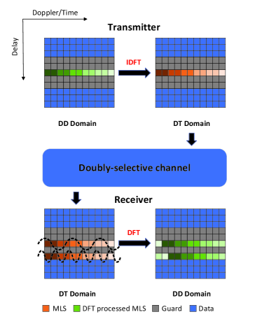
Based on the input-output relationship derived in section II, we can derive the signal expression for the received MLS at the receiver, as illustrated in Fig. 1. According to (3), the MLS in the received DT domain signal will be spread across different rows with delay . Further, the mathematical expression for the sequence in the -th row of the DT grid is given by .
It can be observed that the non-zero rows in the received DT grid are in the form of MLS multiplied by a complex exponential sequence. Therefore, by utilizing the good autocorrelation properties of MLS to locate and obtain , we can complete the estimation of TO and delay.
To locate in the DT domain, we first extract a portion of the received signal that can serve as a row in the DT domain grid. We denote the row as , and use the local MLS to correlate with the corresponding part of . This process can be mathematically represented as .
When locating , we have and . For the bipolar MLS , we have and . Then, we perform an -point DFT on to yield . Since is a complex exponential sequence, the magnitude will exhibit a distinct peak. When is an integer, the peak occurs at , and its value is . According to this principle, the proposed algorithm can detect all paths in the channel.
Next, we analyze the case of not being located accurately, i.e., there is a TO. In this case, we decompose TO as , where and represent delay and time dimensions TO, respectively. When there is a delay dimension TO, i.e., , does not correlate with . As a result, will not exhibit a distinct peak. For the case that only the time-dimension TO exists, i.e., and , the following lemma explains why the proposed algorithm does not require additional time-dimension TO estimation.
Lemma 1.
When and , will not exhibit a distinct peak, i.e.,
| (4) |
Proof.
Please refer to the Appendix. ∎
The above lemma tells that, due to the good autocorrelation properties of MLS, even if is very small, making and nearly identical except for a slight shift, will not exhibit a distinct peak. Therefore, the proposed algorithm does not require additional time-dimension TO estimation.
Based on the above analysis, we can estimate the delay taps and TO by performing normalized threshold detection on the maximum magnitude of DFT of . The detailed steps are summarized in the latter Algorithm 1.
We then discuss how to determine the detection threshold . The value of is determined based on the “non-peak” condition. In the presence of TO, is usually data symbols with . Therefore, and with . According to the central limit theorem, approximately follows a complex Gaussian distribution with zero mean and variance. follows a Rayleigh distribution with mean and variance. Besides, follows a complex Gaussian distribution with mean and variance. Considering the complex Gaussian white noise, the above three distributions still hold, but the value of changes. Given a very small probability , there exist parameters such that . Thus, we can set , where can be obtained experimentally. This value is only related to , i.e., the given probability . Hence, the threshold is applicable to different signal-to-noise ratios (SNRs) and OTFS sizes.
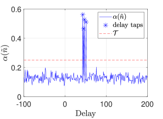
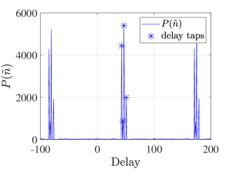
Fig. 2 depicts a snapshot of the timing metric and correlation function , used for TO estimation in the proposed algorithm and [7] respectively. The parameters for OTFS systems are , , data SNR , MLS SNR , pilot SNR [7] . The detection threshold is set reasonably and helps to effectively capture the delay taps, as seen in Fig. 2(a). We can also observe from Figs. 2(a) and 2(b) that the obtained by the proposed algorithm does not exhibit a peak at . As a result, the proposed algorithm does not require additional TO estimation. Further, as observed in Fig. 2(b), the method in [7] suffers from TO estimation errors due to the first path of the channel not being the strongest path. In contrast, the proposed algorithm accurately estimates TO by capturing all paths of the channel.
III-B Doppler & Channel Gain Estimation
After obtaining the TO and channel delay taps, we then estimate the Doppler taps and channel gains. For any path in the channel with delay , let , we have . To estimate the Doppler tap , a direct approach is to estimate it based on the location of the peak in , which is feasible when is an integer. However, when is fractional, spectral leakage will greatly affect accurate estimation of . Given that is a complex exponential sequence, this letter estimates using the following expression: , where denotes the phase angle operation. After obtaining , the estimated gain can be computed by the following close-formed expression: .
Finally, on the basis of the above derivations, we can summarize the main steps of time synchronization and channel estimation in Algorithm 1.
IV Simulation results
In this section, we analyze the performance of the proposed algorithm through simulations. The default system parameters are set as follows: carrier frequency 8 GHz, subcarrier spacing 15 kHz, , , RCP length , detection threshold , and 4-QAM signals. We refer to [3] for the definitions of average data SNR and average MLS SNR . The channel model in [10] is utilized. The maximum speed of a mobile user is set to , corresponding to a maximum Doppler shift index , and we assume a maximum delay index .
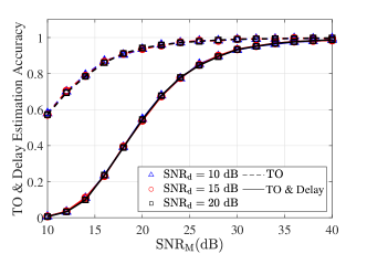
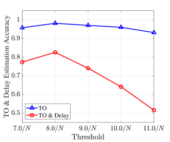
In Fig. 3, we investigate the performance of the designed TO and delay estimation scheme. Specifically, under the condition of , we conduct simulations for each , measuring the performance of the estimation scheme by the proportion of accurately estimated TO and channel delay taps. In Fig. 3, the dashed line represents the proportion of accurately estimated TO, while the solid line represents the proportion of accurately estimated TO and delay taps. The results show that the estimation accuracy is independent of and positively correlated with . This is because the added guard symbols ensure that the data symbols and MLS do not interfere with each other. Further, when , the designed TO and delay estimation scheme achieves accurate TO estimation. Although there are some errors in the delay estimation, it also reaches a high level of accuracy. The sources of error in the delay estimation are twofold: 1) Missed detection: paths with smaller channel gains have correlation peaks below the threshold and are missed. 2) False detection: spurious peaks above the threshold are falsely identified as paths. Missed detection decreases with increasing , while false detection is independent of . Therefore, the high accuracy at indicates that missed detection is the main source of delay estimation error. Paths with smaller channel gains have a relatively minor impact on the accuracy of channel estimation. Thus, the missed detection of these paths is acceptable for the decision process to some extent. This will be verified in the subsequent BER simulations.
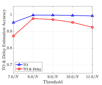
Next, we examine the impact of threshold on the estimation of TO and delay. Fig. 4 illustrates the relationship between estimation accuracy and threshold under conditions of and , respectively. The previous simulation results indicate that the estimation performance is independent of . The following simulations are conducted under the assumption of . The simulation results shown in Fig. 4 reveal that has a significant advantage in low MLS power scenarios and maintains good accuracy under high MLS power conditions. This is because missed detection is more likely to happen at low MLS power levels, where a relatively lower threshold is more beneficial. In summary, for the given system parameters, the optimal threshold approximates .
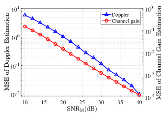
In Fig. 5, we evaluate the performance of the designed Doppler and channel gain estimation scheme. To focus solely on the accuracy of Doppler and channel gain estimation, we assume perfect acquisition of TO and delay information. We assess the mean square error (MSE) performance of the designed Doppler and channel gain estimation scheme and discuss the trend of MSE versus the value of . It can be observed that, similar to delay estimation, as increases, the Doppler and channel gain estimation errors decrease.
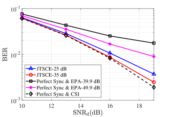
Finally, in Fig. 6, we compare the proposed JTSCE with EPA to evaluate its BER performance. For signal detection, we employ the linear minimum mean-square error (LMMSE) algorithm [9]. To ensure accurate estimation of TO and delays, we set to 25 dB and 35 dB based on the conclusions drawn from Fig. 3. For a fair comparison, we ensure that the total power of the embedded sequences in both algorithms is the same. That is, set the pilot power of EPA to be greater than that of JTSCE. The BER curve with perfect synchronization and CSI is also plotted. Simulation results show that as the power of pilot increases, the BER performance of both algorithms improves, which aligns with the improved accuracy of Doppler and gain estimation observed in Fig. 5. Additionally, when allocating the same pilot power, JTSCE achieves better BER performance than EPA. When reaches 35 dB, the achieved BER of JTSCE is close to that of the case of perfect time synchronization and CSI.
V Conclusion
In this letter, we proposed a joint time synchronization and channel estimation algorithm for OTFS. In this algorithm, we leveraged MLS as pilots to accomplish time synchronization and channel estimation. Initially, we utilized the good autocorrelation properties of the MLS to estimate TO and delay. This approach had the advantage of not requiring additional time-dimension TO estimation and maintaining TO estimation accuracy when the first path in the channel was not the strongest. After determining the starting position of OTFS signal and the delay of each path of the channel, we estimated the Doppler and channel gain for each path. We analyzed the accuracy of the proposed algorithm’s TO and delay estimation performance through simulations, as well as the MSE of Doppler and channel gain estimation. We also evaluated the BER performance, and the results indicated that the proposed algorithm’s BER performance was close to the perfect time synchronization and CSI scenario. Moreover, with the same pilot power, it outperformed the embedded pilot-aided counterpart.
[Proof of Lemma 1] When and , can be expressed as , where represents the interference caused by . does not correlate with . Thus, we consider the case of .
The MLS has the property , for . Therefore, we have
| (5) |
Performing DFT on
| (6) |
we get
| (7) |
When , according to (5), we obtain
| (8) |
Thus, when and , does not exhibit a significant peak.
This completes the proof.
References
- [1] M. H. Abid, I. A. Talin, and M. I. Kadir, “Wavelet-aided OTFS for RIS-assisted high-mobility wireless channels,” IEEE Wireless Communications Letter, vol. 13, no. 6, pp. 1611–1615, 2024.
- [2] A. Singh, S. Sharma, M. Sharma, K. Deka, and D. B. da Costa, “Autoencoder based end-to-end OTFS system design with hardware impairments,” IEEE Wireless Communications Letters, 2024, in Press. DOI 10.1109/LWC.2024.3412240.
- [3] P. Raviteja, K. T. Phan, and Y. Hong, “Embedded pilot-aided channel estimation for OTFS in delay–doppler channels,” IEEE transactions on vehicular technology, vol. 68, no. 5, pp. 4906–4917, 2019.
- [4] W. Yuan, S. Li, Z. Wei, J. Yuan, and D. W. K. Ng, “Data-aided channel estimation for OTFS systems with a superimposed pilot and data transmission scheme,” IEEE wireless communications letters, vol. 10, no. 9, pp. 1954–1958, 2021.
- [5] N. Hashimoto, N. Osawa, K. Yamazaki, and S. Ibi, “Channel estimation and equalization for CP-OFDM-based OTFS in fractional doppler channels,” in 2021 IEEE International Conference on Communications Workshops (ICC Workshops). IEEE, 2021, pp. 1–7.
- [6] Z. Wei, W. Yuan, S. Li, J. Yuan, and D. W. K. Ng, “Off-grid channel estimation with sparse bayesian learning for OTFS systems,” IEEE Transactions on Wireless Communications, vol. 21, no. 9, pp. 7407–7426, 2022.
- [7] M. Bayat and A. Farhang, “Time and frequency synchronization for OTFS,” IEEE Wireless Communications Letters, vol. 11, no. 12, pp. 2670–2674, 2022.
- [8] S. Li, M. Zhang, C. Ju, D. Wang, W. Chen, P. Zhou, and D. Wang, “Downlink carrier frequency offset estimation for OTFS-based LEO satellite communication system,” IEEE Communications Letters, 2023.
- [9] Y. Hong, T. Thaj, and E. Viterbo, Delay-Doppler Communications: Principles and Applications. Academic Press, 2022.
- [10] W. Yuan, Z. Wei, J. Yuan, and D. W. K. Ng, “A simple variational Bayes detector for orthogonal time frequency space (OTFS) modulation,” IEEE transactions on vehicular technology, vol. 69, no. 7, pp. 7976–7980, 2020.