Pinch points and half moons encode Berry curvature
Abstract
“Half moons”, distinctive crescent patterns in the dynamical structure factor, have been identified in inelastic neutron scattering experiments for a wide range of frustrated magnets. In an earlier paper [H. Yan et al., Phys. Rev. B 98, 140402(R) (2018)] we have shown how these features are linked to the local constraints realized in classical spin liquids. Here we explore their implication for the topology of magnon bands. The presence of half moons indicates a separation of magnetic degrees of freedom into irrotational and incompressible components. Where bands satisfying these constraints meet, it is at a singular point encoding Berry curvature of . Interactions which mix the bands open a gap, resolving the singularity, and leading to bands with finite Berry curvature, accompanied by characteristic changes to half–moon motifs. These results imply that inelastic neutron scattering can, in some cases, be used to make rigorous inference about the topological nature of magnon bands.
The realisation that bands of electrons can be classified using topological indices provided both a monumental shock, and an enormous stimulus to research in condensed matter physics. First studied as “Chern Insulators”, in the context of the Integer Quantum Hall effect [1, 2, 3, 4], and later revived in the context of Graphene [5, 6], work on topological bands of electrons has grown to encompass a large and active field of research on topological semi–metals, insulators and superconductors [7, 8]. More recently, magnetic insulators have also entered the stage, through the realization that bands of magnetic excitations can also carry topological indices. A prime example is provided by the “Shastry–Sutherland” magnet SrCu2(BO3)2 [9], where Dzyaloshinski–Moriya interactions both enable triplon excitations to form a dispersing band, and act as a pseudo–magnetic field for these excitations, endowing them with a finite Chern number [10].
Work on topological bands in magnets has evolved into an active subfield in its own right [11, 12, 13, 10, 14, 15, 16, 17, 18, 19, 20, 21, 22, 23, 24, 21, 25, 26, 27, 28, 29, 30, 31, 32, 33, 34, 35, 36, 37, 38, 39, 40, 41], with important themes including the taxonomy of bosonic Chern insulators [21], the analysis of interactions [15, 20, 24], and closing the gap between theory and experiment [42, 43, 44, 45, 46, 47, 18, 48, 49, 50, 51]. This last point, however, presents a serious challenge. In the case of topological insulators, both the quantization of the Hall response, and the character of surface states, provide information about the topology of the underlying electron bands, with surface states easily accessible through tunneling or photoemission experiments [7, 8]. Equivalent surface states exist in topological bands of magnons [13] and triplons [10], but at present there is no established technique for measuring them. Meanwhile, the corresponding thermal Hall and Nernst effects, while sensitive to Berry phases, are not quantized [42, 44, 52], and notoriously difficult to measure. It is therefore of great interest to know whether topological bands of excitations in magnetic insulators have other, more–easily accessible fingerprints in experiment.
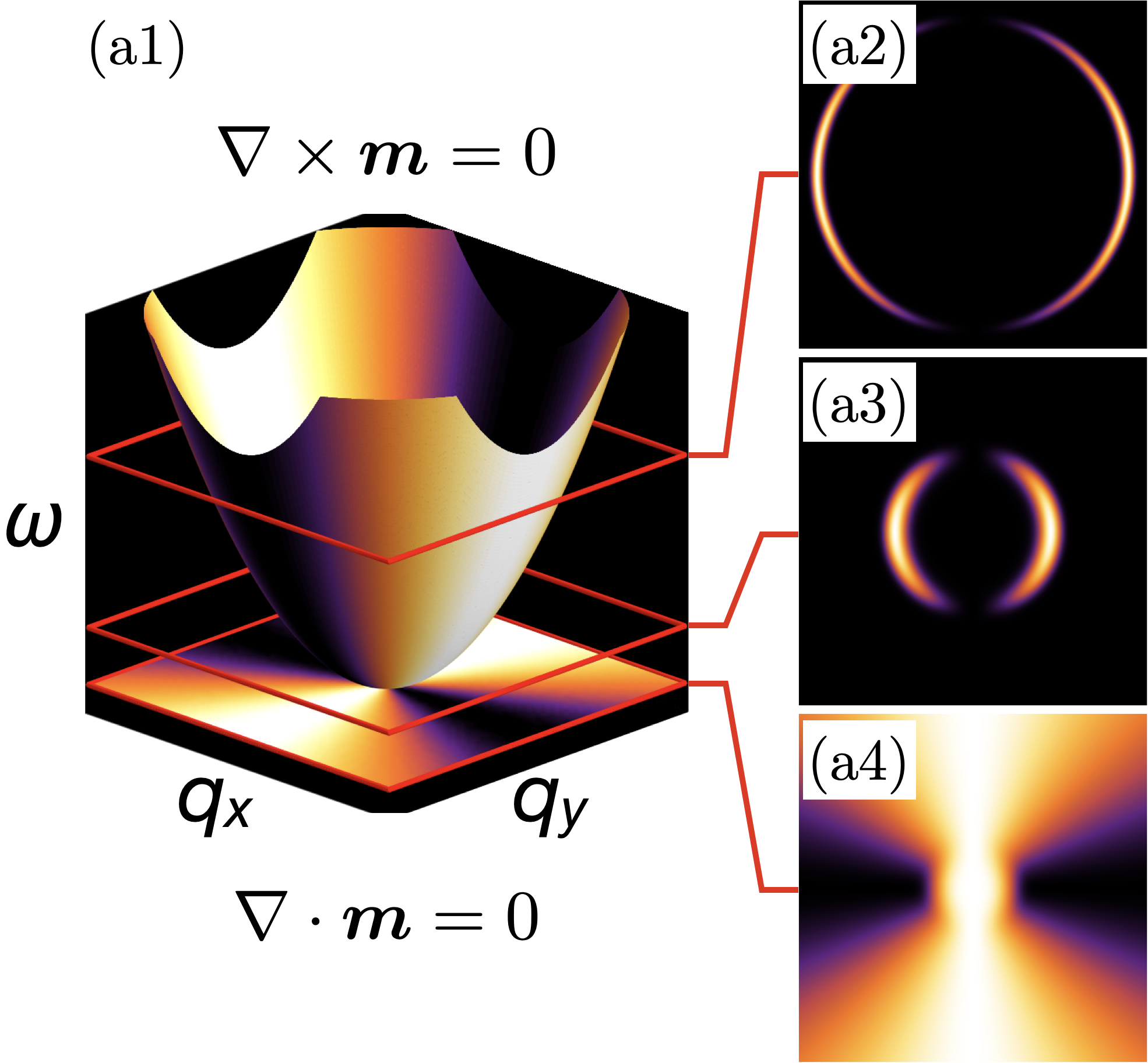
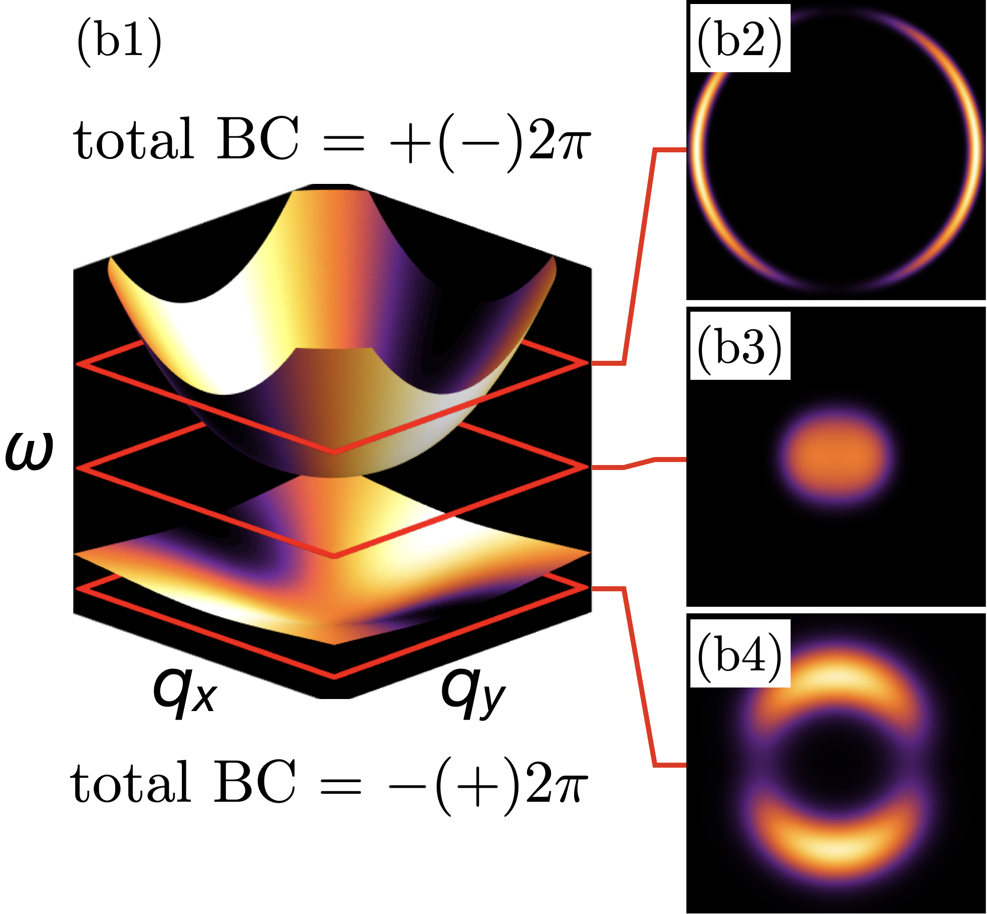
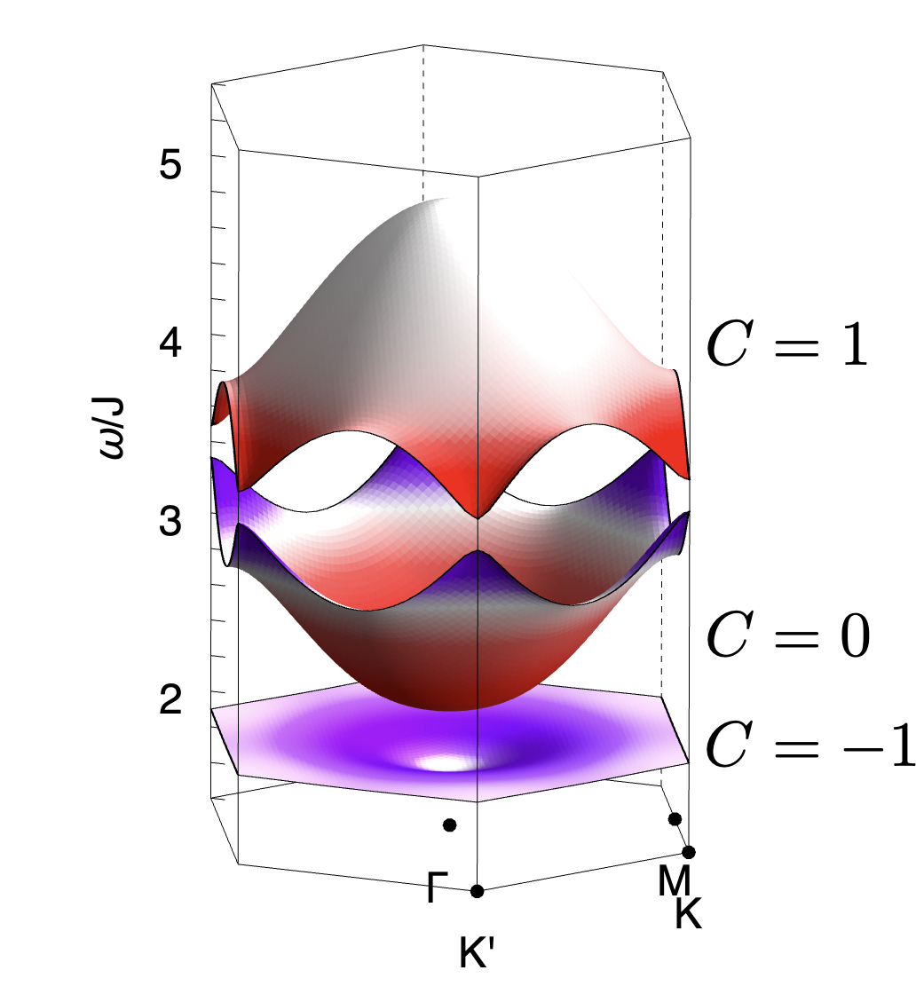
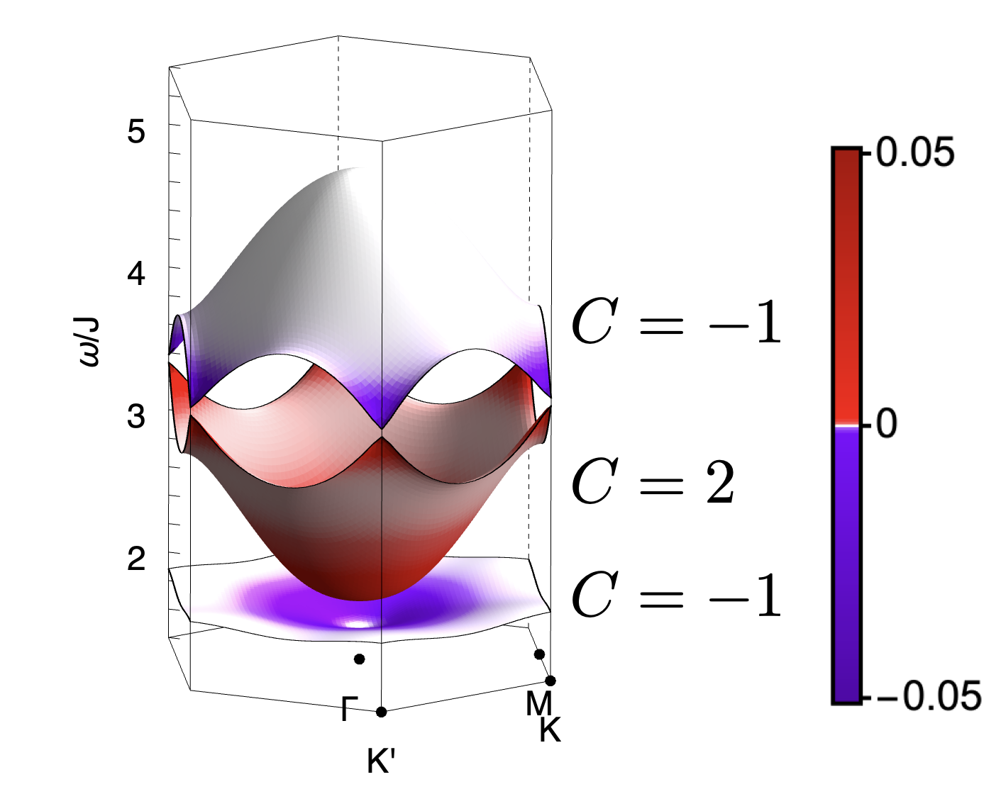
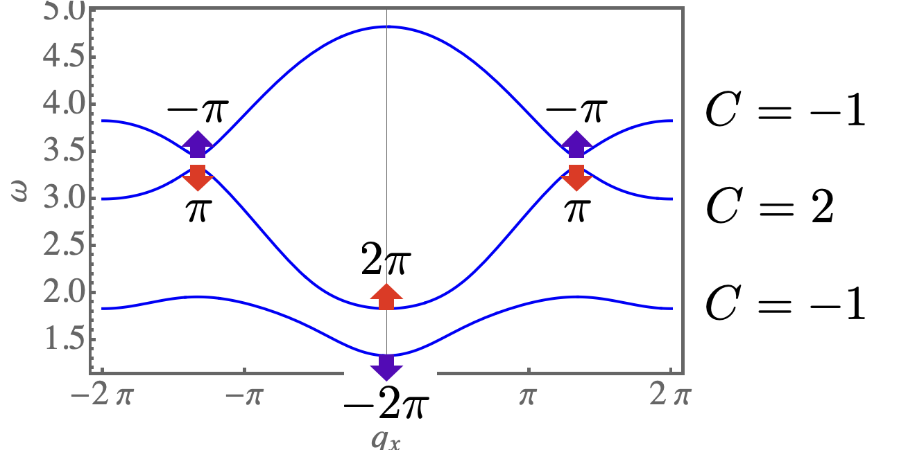
In this Letter, we explore signatures of band–topology which are accesible in conventional, bulk, inelastic neutron scattering, in a broad class of frustrated magnets. Building on earlier work [53, 54], we investigate the interplay between the widely observed “pinch–point” and “half–moon” motifs, and the Berry curvature of associated band–excitations. Pinch–points and half–moons arise as a consequence of “fragmentation” — the separation of magnetic degrees of freedom into components with divergence-free (incompressible) and curl-free (irrotational) character [55, 53]. Where bands with divergence–free and curl–free character meet, pinch–point and half–moon features converge on a singular point with incipient Berry curvature of [Fig. 1a]. If interactions mix states belonging to these two bands, a gap opens, eliminating the singularity, and endowing each band with a Berry curvature . This is accompanied by characteristic changes in pinch–point and half–moon features approaching the avoided band–touching [Fig. 1b]. We demonstrate these effects for magnon bands in a model of spin–1/2 moments on the Kagome–lattice, where anisotropic exchange interactions provide the driving force for band topology. None the less, the resulting phenomenology is very general, and we discuss a range of different candidate systems, developing explicit predictions for the Kagome ferromagnet Cu(1,3-bdc) [56].
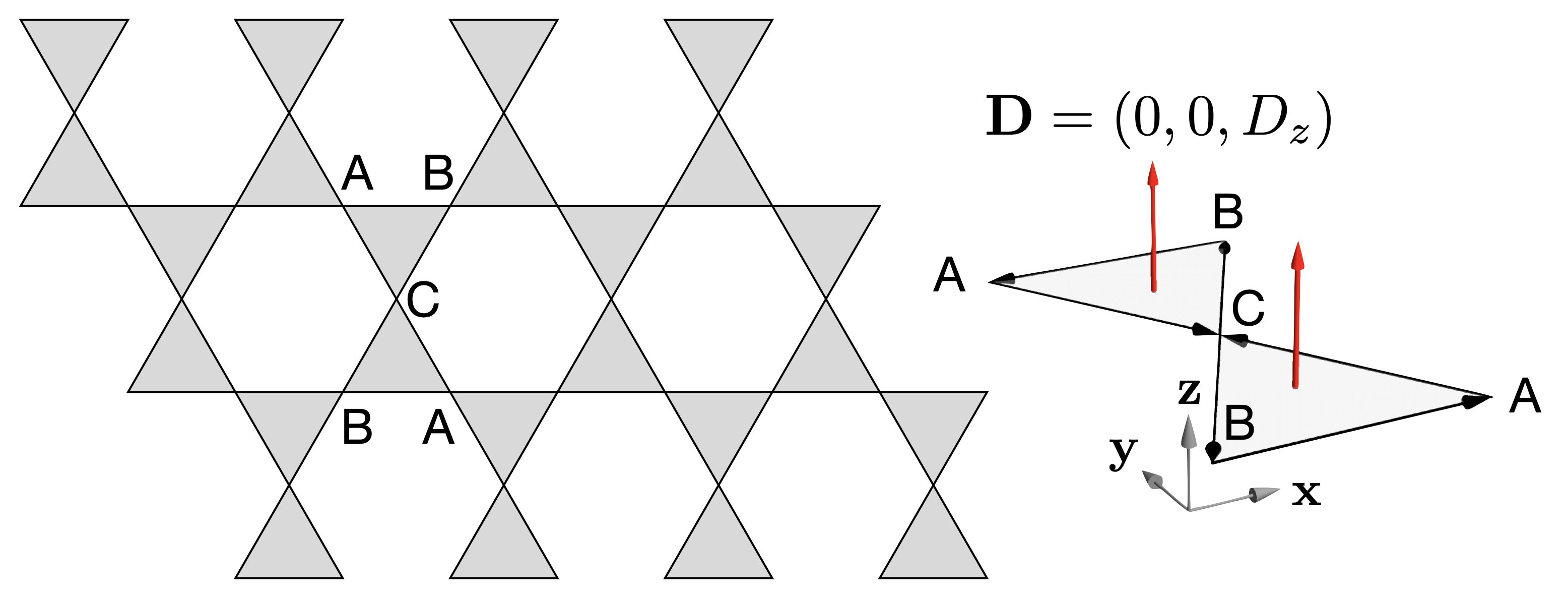
The Model. In magnets, as in systems with itinerant electrons, topological bands usually originate in spin–orbit coupling. This commonly takes the form of Dzyaloshinski–Moriya (DM) interaction with many of the most widely–studied frustrated lattices having a corner–sharing geometry which permits anisotropic exchange, including DM interactions [12, 13, 10, 57, 14, 15, 58, 16, 17, 18, 19, 21, 22, 23, 24]. As a representative example, we consider a spin–1/2 magnet with anisotropic exchange interactions on the first–neighbor bonds of a kagome lattice [Fig. 2]. The point–group symmetry of this lattice is D6h [59, 60], and the existence of a mirror plane restricts anisotropic interactions to transverse spin components, so that the most general model is
| (1) | |||||
where is an applied magnetic field, is a unit vector in the direction of the bond , and
| (2) |
. In what follows we will emphasize DM interactions , setting and . None the less, the conclusions we reach about the relationship between “half moons” and Berry curvature are completely general, and hold regardless of which type of anisotropy is considered. A complete analysis, including , is given in the Supplemental Material.
We focus on single–magnon excitations about a state where spins are collinear, either because of FM exchange interactions or because they have been polarised by magnetic field . For sufficiently large spin–wave gap (guaranteed by high magnetic field), these will be well–described by a non–interacting theory [62, 15, 20, 24], which we can access through the equation of motion (EoM) for the magnon creation operator
| (3) |
where is the band index, and all information about band topology is encoded in .
Symmetry analysis and Helmholtz decomposition. In order to make connection with singular features in scattering (half moons), we now decompose magnetic excitations into incompressible (divergence–free) and irrotational (curl–free) components. It is convenient to start from irreducible representations (irreps) of spins on the triangular units which form the building–blocks of the Kagome lattice
| (4a) | |||||
| (4b) | |||||
where the convention for labelling lattice sites is given in Fig. 2. In the long–wavelength limit (), this allows us to describe magnons, Eq (3), in terms of fields and . We then employ the Helmholtz–Hodge decomposition [63], writing
| (5) |
where , , and is the two-dimensional curl. From the Heisenberg EoM we find
| (6a) | ||||
| (6b) | ||||
where , , and we set .
Origin of half moons. In the absence of anisotropic exchange interactions, i.e. for , excitations with incompressible and irrotational character are entirely decoupled [53, 64]. Solving Eq. (6a) by Fourier transformation , we find a flat band of incompressible excitations
| (7) |
with corresponding eigenvector
| (8) |
Meanwhile, making use of the identity , we can solve Eq. (6b) to find a quadratically–dispersing band of irrotational excitations
| (9) |
with eigenvector
| (10) |
For the two bands are degenerate, and touch quadratically.
We are now in a position to calculate dynamical structure factors. Writing we find
where indexes the irrotational and incompressible modes, respectively; ;
| (12) |
and, for , .
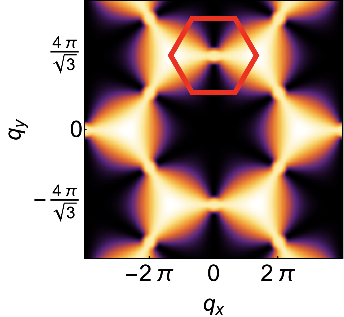
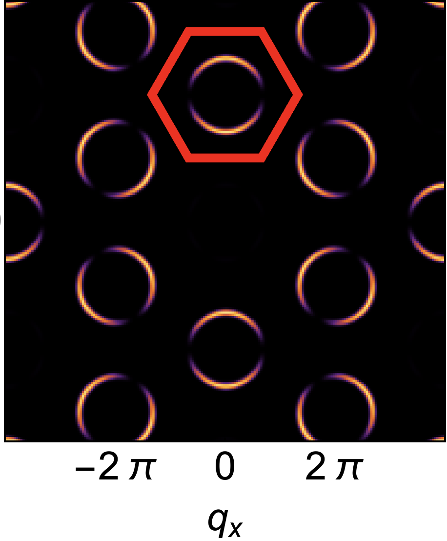
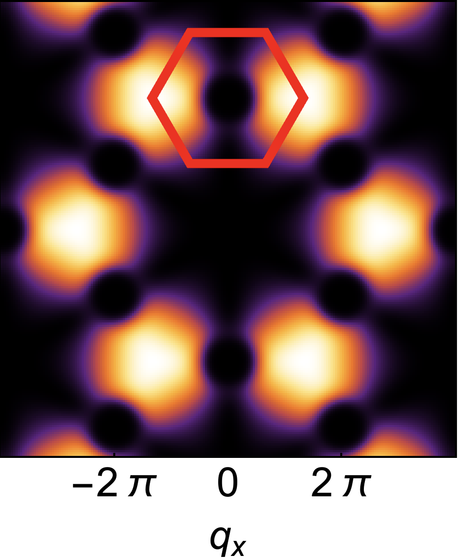
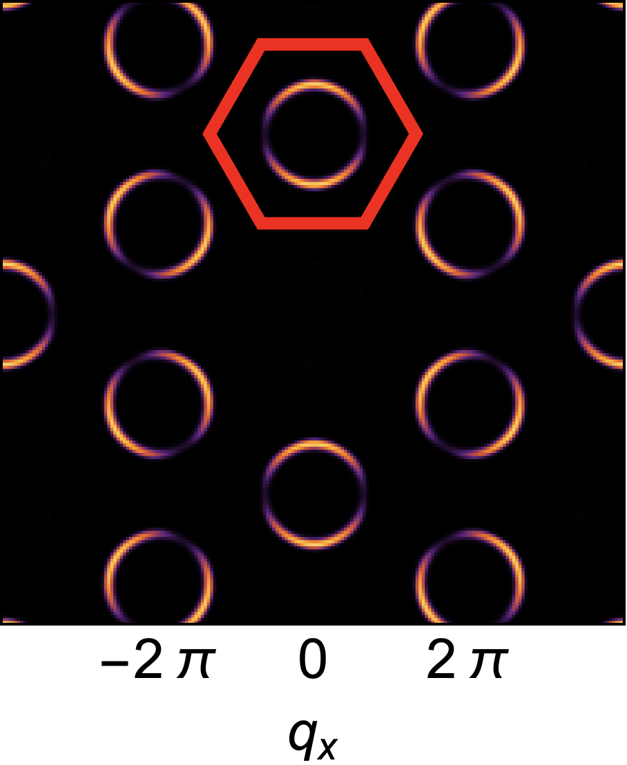
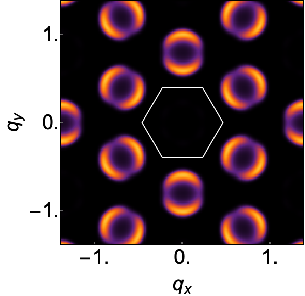
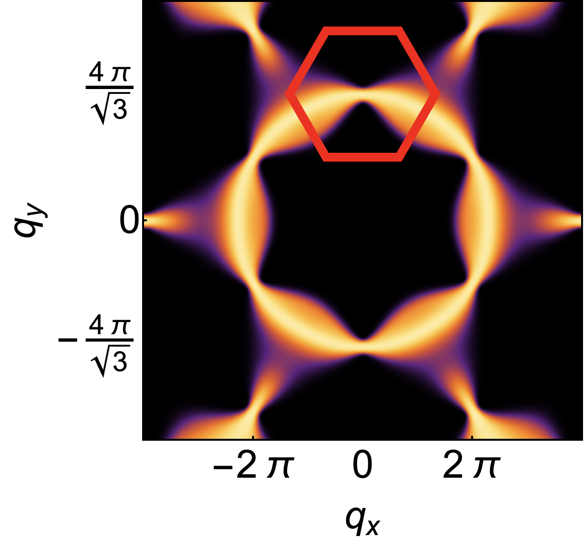
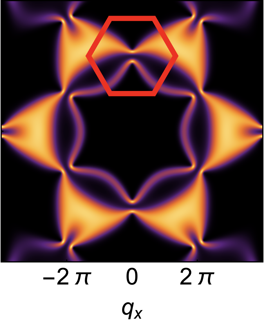
For , the limit is a function of , and therefore singular. This form of singularity is well–known in the context of spin–liquids, where it is referred to as a “pinch–point” [65, 53, 66]. For the flat band associated with incompressible excitations, the pinch point is directly visible in the dynamical structure factor at [53, 64]. Meanwhile, for the dispersing band of irrotational excitations, the pinch–point manifests as crescent–shaped “half–moons” in constant–energy cuts for [53]. These effects are illustrated schematically in Fig. 1a. 222Here and in Fig. 3, singular behaviour for is obscured by the finite energy resolution used in making plots of ..
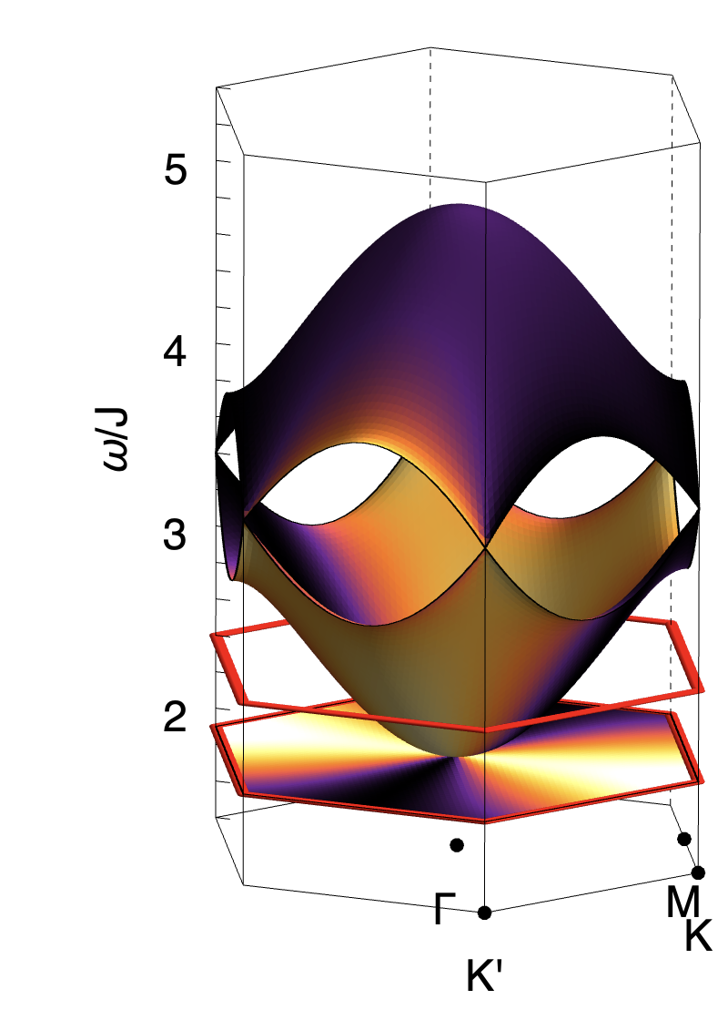
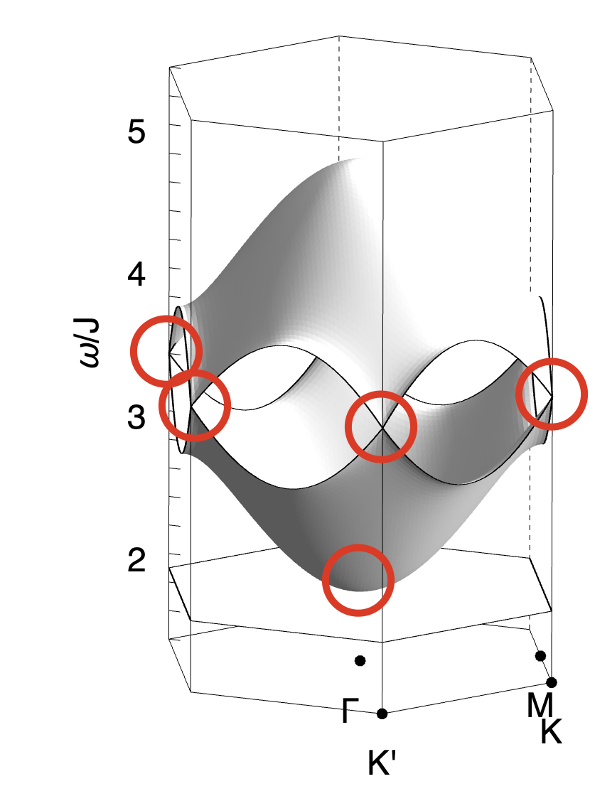
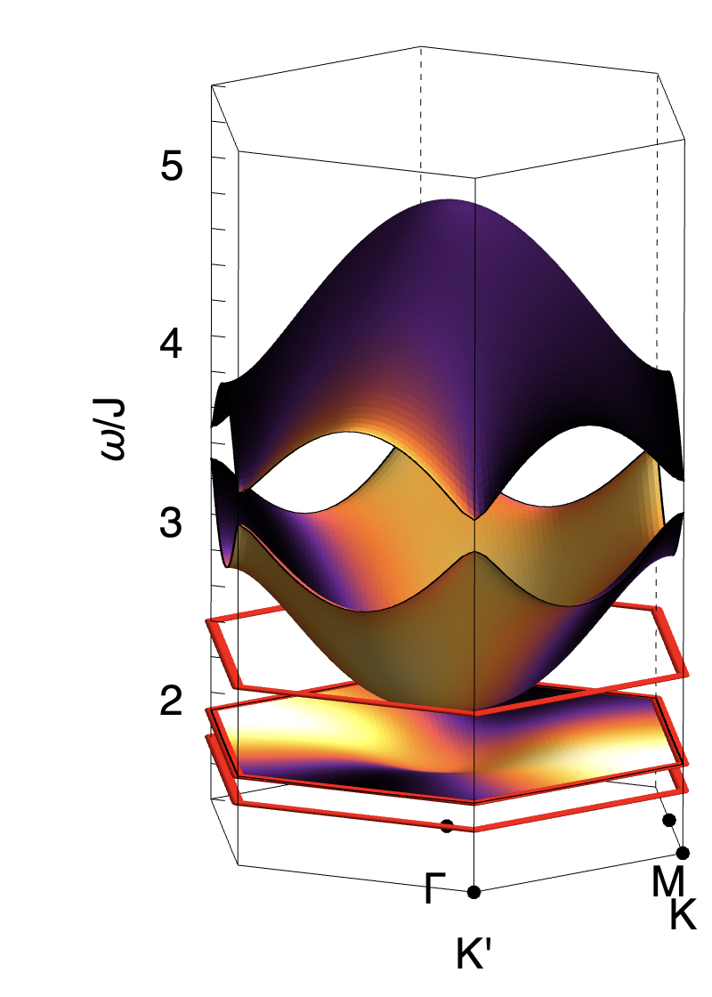
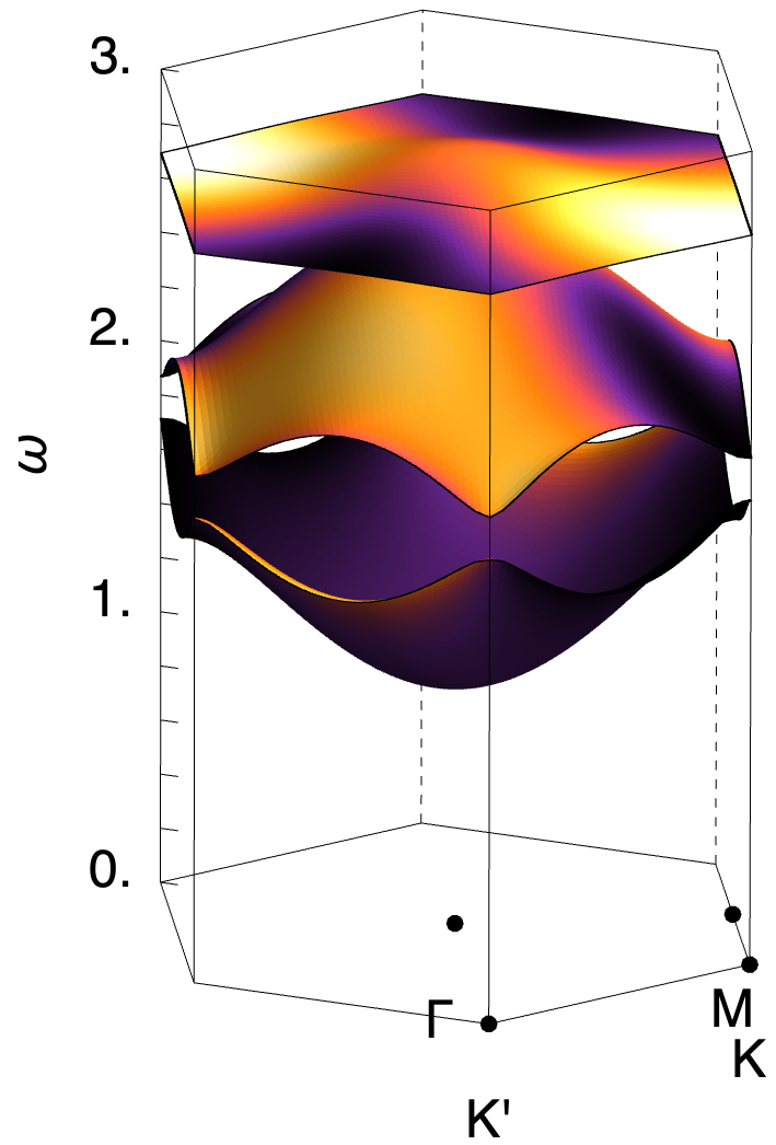
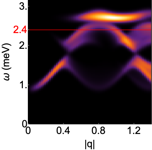
Exactly the same phenomenology is found in direct calculations from the microscopic model Eq. (1). In Fig. 3 we present results of linear spin wave (LSW) theory, showing the flat band and dispersing bands found for , , [Fig. 3a]. The pinch point on the flat band is exhibited in Fig. 3e, while half moons associated with the dispersing band are shown in Fig. 3f. Details of these calculations are given in the Supplemental Materials.
Opening of gap and elimination of singularity. The new feature which arises in the presence of anisotropic exchange interactions is the mixing of incompressible and irrotational excitations. Solving Eq. (6a), Eq. (6b) for , we find that the quadratic band–touching at is replaced by a gap
| (13) |
between bands with dispersion
| (14) |
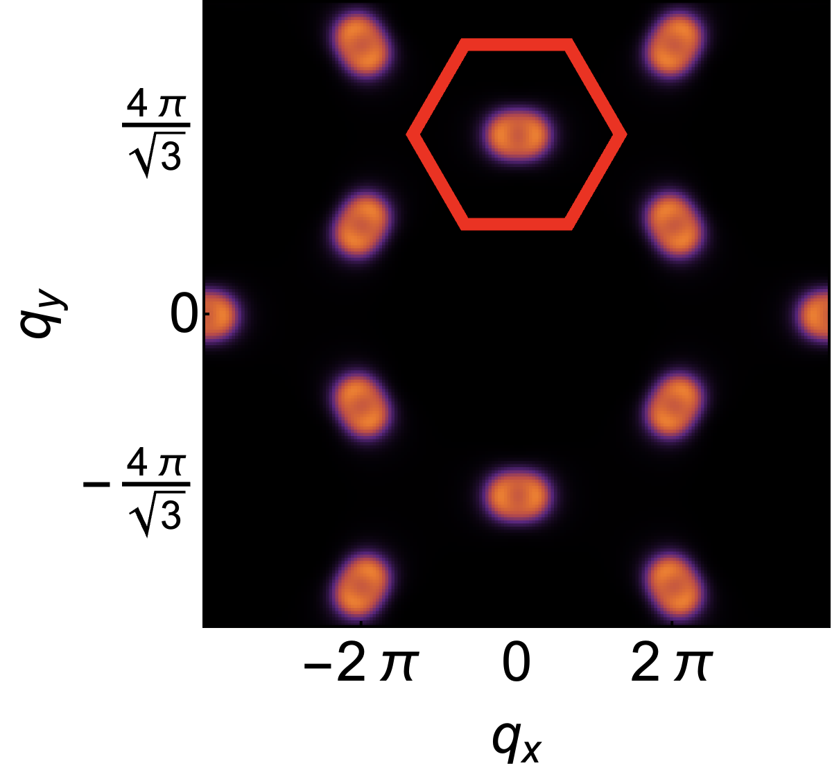
Hybridization also eliminates singular correlations for ; the dynamical structure factor is given by Eq. (LABEL:eq:S.q.omega), but with
| (15) |
where determines the scale at which correlations cross over from a pinch–point structure at large , to a non–singular behaviour for .
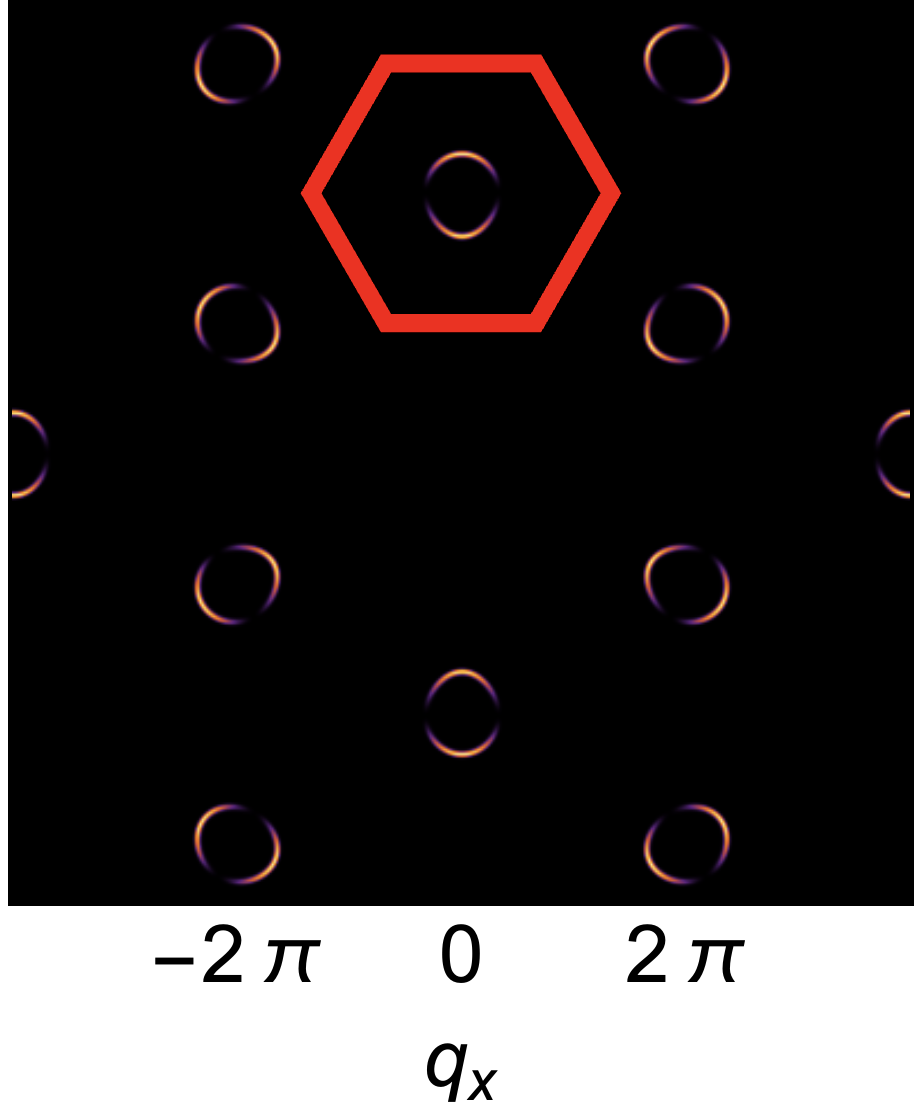
As a consequence the pinch–points (half–moons) observed for , vanish for . None the less, half–moon features remain visible for , and can also be resolved on the formerly–flat band associated with incompressible excitations, as a consequence of its finite dispersion. This phenomenology is illustrated schematically in Fig. 1b, and for LSW calculations in Fig. 3c and Fig. 3g–3i
Berry phase effects and band–topology. The Helmholtz decomposition, Eq. (5) also has important implications for band topology. In the absence anisotropic exchange interactions, each of the eigenvectors Eq. (8) and Eq. (10), winds exactly once about the singular point, . As a consequence, their quadratic band–touching is topologically critical, encoding Berry curvature of at the singularity. Introducing an interaction which mixes excitations with incompressible and irrotational character, such as , resolves the singularity at , opening a gap, and injecting Berry curvature of into each band.
We can explore these effects in more detail by noting that the EoM, Eq. (6), describe an effective two–level system
| (16) |
where is a identity matrix, is a vector of Pauli matrices, , and
| (17) |
The Berry curvature associated with is
| (18) |
This curvature integrates to , and is concentrated in the vicinity of . In the absence of other sources of Berry curvature, this will endow magnon bands with integer Chern number . This phenomenology, linked to a quadratic band–touching, should be contrasted with the widely–studied case of linear band–crossings (Dirac cones), which encode Berry curvature [68].
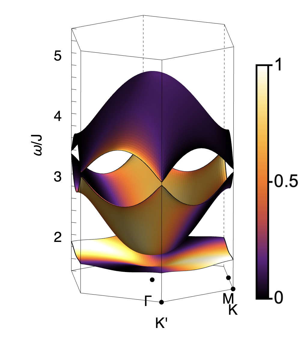
It is also possible to calculate both Berry curvature and Chern numbers within LSW theory. Results for are shown in Fig. 3d. Once the third band is taken into account, magnon bands also receive a net contribution of Berry phase from the linear band–crossings at and [Fig. 3b]. For , , this leads to bands with Chern numbers .
![[Uncaptioned image]](https://cdn.awesomepapers.org/papers/457912d8-1630-44bf-9599-2566380efa94/Fig4-Legend.png)
Inference of Berry Curvature from spectral features. We now address the question of what we could have inferred about the topology of magnon bands from universal features in alone. In a model with only two Magnon bands, the observation of half–moons approaching an avoided band–touching would be enough to completely characterise band topology, up to the sign of Chern numbers . However the Kagome–lattice model we consider supports three band of magnons, and we must also take into account contributions to Berry phase coming from the third band; in particular the linear band–crossings at and .
The universal features associated with linear band–crossings are already well–characterised, comprising a single arc in , which swaps orientation above and below the (avoided) band–touching point [70]. This phenomenology can be found in LSW calculations for Eq. (1), described in the [Supplemental Materials], and it is possible to infer Berry curvature at and from spectral features near these points.
Combining these results, we can safely infer the existence of topological magnon bands in the Kagome lattice model, Eq. (1), from spectral features alone 333An alternative line of reasoning, leading to the same conclusion, is given in Ref. 60.. None the less, the sign of the contribution to Berry phase coming from each band–touching/bond–crossing point depends on details of interactions, and cannot be inferred solely from the existence of half–moons/arcs in . For this reason, additional information is required to assign a unique set of Chern numbers to these bands. This could sought from thermal Hall measurements, which are sensitive to the sign of Berry curvature [42, 44] or, where models are sufficiently well–constrained, from fits to non–universal features in scattering.
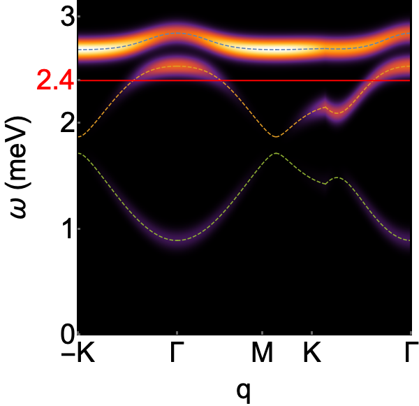
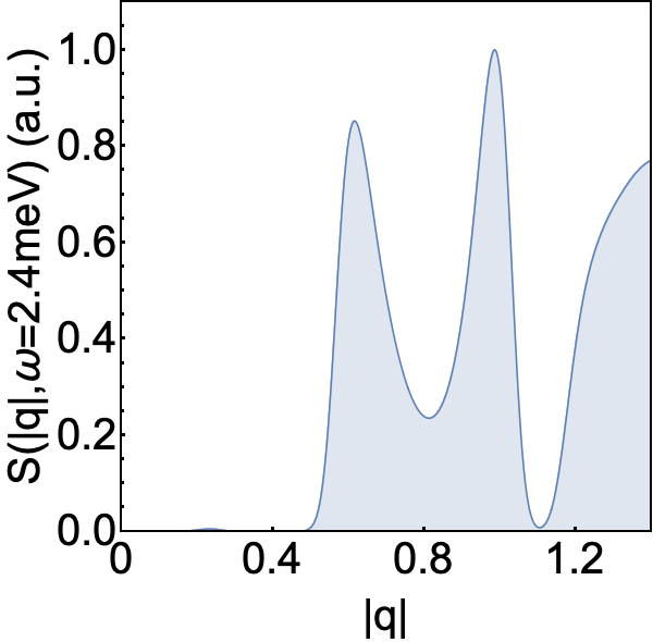
Application to experiment. A wide range of frustrated magnets are candidates for topological band structure, and we now consider what might be learned from half moon features observed in inelastic neutron scattering. One example is Cu(1,3-bdc), a layered metal–organic framework (MOF) which realises a structurally–perfect Kagome lattice [72]. Neutron scattering experiments on Cu(1,3-bdc) [69] reveal a ferromagnetic (FM) ground state, and dispersing magnon bands which are well–described by model with first–neighbour FM exchange and DM interactions. In Fig. 4c we present LSW predictions for Cu(1,3-bdc), for parameters taken from experiment. Half–moon features are resolved near to an avoided band–touching at . These lead to a characteristic double peak in predictions for the angle–integrated structure factor , providing a sharp experimental signature of Berry phase within the magnon bands.
The bilayer breathing Kagome magnet Ca10Cr7O28 [73] is also of note. This system has a mixture of FM and AF interactions; saturates at a magnetic field of approximately ; and is well–described by a model which supports pinch–point and half moon features [74]. The pyrochlore magnet Lu2V2O7 is another strong candidate, and features redolant of half–moons, approaching a flat band, have already been observed in experiment [75].
Another interesting avenue to explore would be correlations within topological bands of electrons. The phenomenology of half moons and Chern numbers developed in this Letter applies equally to electrons, and “Kagome metals” such as Fe3Sn2 [76] and CoSn [77] are already under study; similar topological bands are argued to be possible in conducting MOF’s [78]. In this context, it would be interesting to revisit, for example, ARPES experiments on CoSn [77], where a flat band is observed a little below the Fermi energy, and reinterpret data in the terms of [Eq. (LABEL:eq:S.q.omega)].
Conclusions. Topological bands of excitations are a ubiquitous feature of systems with both itinerant and localised electrons, originating in the Berry curvature of the underlying band states. In this Letter, we have shown that the existence of pinch–points and half–moons in dynamical structure factors approaching an (avoided) quadratic band–touching point guarantees a net source of Berry curvature . The link between Berry curvature and spectral features is provided by the effective two–level model, Eq. (16), which describes the coupling between excitations with incompressible and irrorational character, and is characterised by a vector [Eq. (18)], that winds twice around the band–touching point. These results imply a robust connection between singular features in scattering and Berry curvature [Fig. 1] which can, in some cases, be used to unambiguously determine the topological nature of bands from spectral features alone. This picture is applicable to magnon bands in a wide range of frustrated magnets, and is also relevant to topological bands of electrons on frustrated lattices [79].
Acknowledgements. This work was supported by the Theory of Quantum Matter Unit, Okinawa Institute of Science and Technology Graduate University (OIST). The authors would like to thank Bella Lake and Matthias Gohlke for helpful discussions. H.Y. is supported by the Theory of Quantum Matter Unit at Okinawa Institute of Science and Technology, the Japan Society for the Promotion of Science (JSPS) Research Fellowships for Young Scientists, and the National Science Foundation Division of Materials Research under the Award DMR-191751 at different stages of this project. J. R. was supported by the NSF through grant DMR-2142554.
References
- Klitzing et al. [1980] K. v. Klitzing, G. Dorda, and M. Pepper, New method for high-accuracy determination of the fine-structure constant based on quantized hall resistance, Phys. Rev. Lett. 45, 494 (1980).
- Laughlin [1981] R. B. Laughlin, Quantized hall conductivity in two dimensions, Phys. Rev. B 23, 5632 (1981).
- Thouless et al. [1982] D. J. Thouless, M. Kohmoto, M. P. Nightingale, and M. den Nijs, Quantized hall conductance in a two-dimensional periodic potential, Phys. Rev. Lett. 49, 405 (1982).
- Haldane [1988] F. D. M. Haldane, Model for a quantum hall effect without landau levels: Condensed-matter realization of the ”parity anomaly”, Phys. Rev. Lett. 61, 2015 (1988).
- Kane and Mele [2005a] C. L. Kane and E. J. Mele, Quantum spin hall effect in graphene, Phys. Rev. Lett. 95, 226801 (2005a).
- Kane and Mele [2005b] C. L. Kane and E. J. Mele, topological order and the quantum spin hall effect, Phys. Rev. Lett. 95, 146802 (2005b).
- Hasan and Kane [2010] M. Z. Hasan and C. L. Kane, Colloquium: Topological insulators, Rev. Mod. Phys. 82, 3045 (2010).
- Qi and Zhang [2011] X.-L. Qi and S.-C. Zhang, Topological insulators and superconductors, Rev. Mod. Phys. 83, 1057 (2011).
- Kageyama et al. [1999] H. Kageyama, K. Yoshimura, R. Stern, N. V. Mushnikov, K. Onizuka, M. Kato, K. Kosuge, C. P. Slichter, T. Goto, and Y. Ueda, Exact dimer ground state and quantized magnetization plateaus in the two-dimensional spin system , Phys. Rev. Lett. 82, 3168 (1999).
- Romhányi et al. [2015] J. Romhányi, K. Penc, and R. Ganesh, Hall effect of triplons in a dimerized quantum magnet, Nat Commun 6, 6805 EP (2015).
- Shindou et al. [2013] R. Shindou, R. Matsumoto, S. Murakami, and J.-i. Ohe, Topological chiral magnonic edge mode in a magnonic crystal, Phys. Rev. B 87, 174427 (2013).
- Mook et al. [2014a] A. Mook, J. Henk, and I. Mertig, Magnon hall effect and topology in kagome lattices: A theoretical investigation, Phys. Rev. B 89, 134409 (2014a).
- Mook et al. [2014b] A. Mook, J. Henk, and I. Mertig, Edge states in topological magnon insulators, Phys. Rev. B 90, 024412 (2014b).
- Owerre [2016] S. Owerre, A first theoretical realization of honeycomb topological magnon insulator, Journal of Physics: Condensed Matter 28, 386001 (2016).
- Chernyshev and Maksimov [2016] A. L. Chernyshev and P. A. Maksimov, Damped topological magnons in the kagome-lattice ferromagnets, Phys. Rev. Lett. 117, 187203 (2016).
- Zyuzin and Kovalev [2016] V. A. Zyuzin and A. A. Kovalev, Magnon spin nernst effect in antiferromagnets, Phys. Rev. Lett. 117, 217203 (2016).
- Kim et al. [2016] S. K. Kim, H. Ochoa, R. Zarzuela, and Y. Tserkovnyak, Realization of the haldane-kane-mele model in a system of localized spins, Phys. Rev. Lett. 117, 227201 (2016).
- McClarty et al. [2017] P. A. McClarty, F. Krüger, T. Guidi, S. F. Parker, K. Refson, A. W. Parker, D. Prabhakaran, and R. Coldea, Topological triplon modes and bound states in a shastry–sutherland magnet, Nature Physics 13, 736 (2017).
- Nakata et al. [2017] K. Nakata, J. Klinovaja, and D. Loss, Magnonic quantum hall effect and wiedemann-franz law, Phys. Rev. B 95, 125429 (2017).
- McClarty et al. [2018] P. A. McClarty, X.-Y. Dong, M. Gohlke, J. G. Rau, F. Pollmann, R. Moessner, and K. Penc, Topological magnons in kitaev magnets at high fields, Phys. Rev. B 98, 060404 (2018).
- Kondo et al. [2019] H. Kondo, Y. Akagi, and H. Katsura, Three-dimensional topological magnon systems, Phys. Rev. B 100, 144401 (2019).
- Joshi and Schnyder [2019] D. G. Joshi and A. P. Schnyder, Z 2 topological quantum paramagnet on a honeycomb bilayer, Physical Review B 100, 020407 (2019).
- Romhányi [2019] J. Romhányi, Multipolar edge states in the anisotropic kagome antiferromagnet, Phys. Rev. B 99, 014408 (2019).
- McClarty and Rau [2019] P. A. McClarty and J. G. Rau, Non-hermitian topology of spontaneous magnon decay, Phys. Rev. B 100, 100405 (2019).
- Kawano and Hotta [2019] M. Kawano and C. Hotta, Thermal hall effect and topological edge states in a square-lattice antiferromagnet, Phys. Rev. B 99, 054422 (2019).
- Mook et al. [2019] A. Mook, J. Henk, and I. Mertig, Thermal hall effect in noncollinear coplanar insulating antiferromagnets, Phys. Rev. B 99, 014427 (2019).
- Malki and Uhrig [2020] M. Malki and G. S. Uhrig, Topological magnetic excitations, Europhysics Letters 132, 20003 (2020).
- Bhowmick and Sengupta [2020] D. Bhowmick and P. Sengupta, Antichiral edge states in heisenberg ferromagnet on a honeycomb lattice, Phys. Rev. B 101, 195133 (2020).
- Aguilera et al. [2020] E. Aguilera, R. Jaeschke-Ubiergo, N. Vidal-Silva, L. E. F. F. Torres, and A. S. Nunez, Topological magnonics in the two-dimensional van der waals magnet , Phys. Rev. B 102, 024409 (2020).
- Kondo et al. [2020] H. Kondo, Y. Akagi, and H. Katsura, Non-Hermiticity and topological invariants of magnon Bogoliubov–de Gennes systems, Progress of Theoretical and Experimental Physics 2020, 10.1093/ptep/ptaa151 (2020), 12A104, https://academic.oup.com/ptep/article-pdf/2020/12/12A104/35937396/ptaa151.pdf .
- Mook et al. [2021] A. Mook, K. Plekhanov, J. Klinovaja, and D. Loss, Interaction-stabilized topological magnon insulator in ferromagnets, Phys. Rev. X 11, 021061 (2021).
- Kondo and Akagi [2021] H. Kondo and Y. Akagi, Dirac surface states in magnonic analogs of topological crystalline insulators, Phys. Rev. Lett. 127, 177201 (2021).
- Zhuo et al. [2021] F. Zhuo, H. Li, and A. Manchon, Topological phase transition and thermal hall effect in kagome ferromagnets, Phys. Rev. B 104, 144422 (2021).
- Thomasen et al. [2021] A. Thomasen, K. Penc, N. Shannon, and J. Romhányi, Fragility of topological invariant characterizing triplet excitations in a bilayer kagome magnet, Phys. Rev. B 104, 104412 (2021).
- Kondo and Akagi [2022] H. Kondo and Y. Akagi, Nonlinear magnon spin nernst effect in antiferromagnets and strain-tunable pure spin current, Phys. Rev. Research 4, 013186 (2022).
- Neumann et al. [2022] R. R. Neumann, A. Mook, J. Henk, and I. Mertig, Thermal hall effect of magnons in collinear antiferromagnetic insulators: Signatures of magnetic and topological phase transitions, Phys. Rev. Lett. 128, 117201 (2022).
- Xing et al. [2022] Y. Xing, H. Chen, N. Xu, X. Li, and L. Zhang, Valley modulation and single-edge transport of magnons in breathing kagome ferromagnets, Phys. Rev. B 105, 104409 (2022).
- Chen et al. [2022] Q.-H. Chen, F.-J. Huang, and Y.-P. Fu, Magnon valley thermal hall effect in triangular-lattice antiferromagnets, Phys. Rev. B 105, 224401 (2022).
- Zhuo et al. [2022] F. Zhuo, H. Li, and A. Manchon, Topological thermal hall effect and magnonic edge states in kagome ferromagnets with bond anisotropy, New Journal of Physics 24, 023033 (2022).
- Fujiwara et al. [2022] K. Fujiwara, S. Kitamura, and T. Morimoto, Thermal hall responses in frustrated honeycomb spin systems, Phys. Rev. B 106, 035113 (2022).
- McClarty [2022] P. A. McClarty, Topological magnons: A review, Annual Review of Condensed Matter Physics 13, 171 (2022), https://doi.org/10.1146/annurev-conmatphys-031620-104715 .
- Katsura et al. [2010] H. Katsura, N. Nagaosa, and P. A. Lee, Theory of the thermal hall effect in quantum magnets, Phys. Rev. Lett. 104, 066403 (2010).
- Onose et al. [2010] Y. Onose, T. Ideue, H. Katsura, Y. Shiomi, N. Nagaosa, and Y. Tokura, Observation of the magnon hall effect, Science 329, 297 (2010).
- Matsumoto and Murakami [2011a] R. Matsumoto and S. Murakami, Rotational motion of magnons and the thermal hall effect, Phys. Rev. B 84, 184406 (2011a).
- Ideue et al. [2012] T. Ideue, Y. Onose, H. Katsura, Y. Shiomi, S. Ishiwata, N. Nagaosa, and Y. Tokura, Effect of lattice geometry on magnon Hall effect in ferromagnetic insulators, Phys. Rev. B 85, 134411 (2012).
- Matsumoto et al. [2014] R. Matsumoto, R. Shindou, and S. Murakami, Thermal Hall effect of magnons in magnets with dipolar interaction, Phys. Rev. B 89, 054420 (2014).
- Hirschberger et al. [2015] M. Hirschberger, J. W. Krizan, R. J. Cava, and N. P. Ong, Large thermal hall conductivity of neutral spin excitations in a frustrated quantum magnet, Science 348, 106 (2015), https://www.science.org/doi/pdf/10.1126/science.1257340 .
- Cai et al. [2021] Z. Cai, S. Bao, Z.-L. Gu, Y.-P. Gao, Z. Ma, Y. Shangguan, W. Si, Z.-Y. Dong, W. Wang, Y. Wu, D. Lin, J. Wang, K. Ran, S. Li, D. Adroja, X. Xi, S.-L. Yu, X. Wu, J.-X. Li, and J. Wen, Topological magnon insulator spin excitations in the two-dimensional ferromagnet , Phys. Rev. B 104, L020402 (2021).
- Zhang et al. [2021] H. Zhang, C. Xu, C. Carnahan, M. Sretenovic, N. Suri, D. Xiao, and X. Ke, Anomalous thermal hall effect in an insulating van der waals magnet, Phys. Rev. Lett. 127, 247202 (2021).
- Scheie et al. [2022] A. Scheie, P. Laurell, P. A. McClarty, G. E. Granroth, M. B. Stone, R. Moessner, and S. E. Nagler, Dirac magnons, nodal lines, and nodal plane in elemental gadolinium, Phys. Rev. Lett. 128, 097201 (2022).
- Suetsugu et al. [2022] S. Suetsugu, T. Yokoi, K. Totsuka, T. Ono, I. Tanaka, S. Kasahara, Y. Kasahara, Z. Chengchao, H. Kageyama, and Y. Matsuda, Intrinsic suppression of the topological thermal hall effect in an exactly solvable quantum magnet, Phys. Rev. B 105, 024415 (2022).
- Matsumoto and Murakami [2011b] R. Matsumoto and S. Murakami, Rotational motion of magnons and the thermal hall effect, Phys. Rev. B 84, 184406 (2011b).
- Yan et al. [2018] H. Yan, R. Pohle, and N. Shannon, Half moons are pinch points with dispersion, Phys. Rev. B 98, 140402 (2018).
- Mizoguchi et al. [2018] T. Mizoguchi, L. D. C. Jaubert, R. Moessner, and M. Udagawa, Magnetic clustering, half-moons, and shadow pinch points as signals of a proximate coulomb phase in frustrated heisenberg magnets, Phys. Rev. B 98, 144446 (2018).
- Brooks-Bartlett et al. [2014] M. E. Brooks-Bartlett, S. T. Banks, L. D. Jaubert, A. Harman-Clarke, and P. C. Holdsworth, Magnetic-moment fragmentation and monopole crystallization, Phys. Rev. X 4, 011007 (2014).
- Chisnell et al. [2015a] R. Chisnell, J. S. Helton, D. E. Freedman, D. K. Singh, R. I. Bewley, D. G. Nocera, and Y. S. Lee, Topological magnon bands in a kagome lattice ferromagnet, Phys. Rev. Lett. 115, 147201 (2015a).
- Chernyshev and Zhitomirsky [2015] A. L. Chernyshev and M. E. Zhitomirsky, Order and excitations in kagome-lattice antiferromagnets, Phys. Rev. B 92, 144415 (2015).
- Maksimov and Chernyshev [2016] P. A. Maksimov and A. L. Chernyshev, Field-induced dynamical properties of the model on a honeycomb lattice, Phys. Rev. B 93, 014418 (2016).
- Essafi et al. [2017] K. Essafi, O. Benton, and L. D. C. Jaubert, Generic nearest-neighbor kagome model: Xyz and dzyaloshinskii-moriya couplings with comparison to the pyrochlore-lattice case, Phys. Rev. B 96, 205126 (2017).
- Thomasen [2021] A. Thomasen, Topology of band–like excitations in frustrated magnets and their experimental signatures, Ph.D. thesis, Okinawa Institute of Science and Technology Graudate Univsersity (2021).
- Note [1] This parameterisation of interactions is exactly equivalent to that given in [59, 60], with in Eq. (1) playing the role of in [59, 60].
- MacDonald et al. [1988] A. H. MacDonald, S. M. Girvin, and D. Yoshioka, expansion for the hubbard model, Phys. Rev. B 37, 9753 (1988).
- Arfken and Weber [1995] G. B. Arfken and H. J. Weber, Mathematical Methods for Physicists (Academic Press: San Diego, 1995).
- Benton [2016] O. Benton, Quantum origins of moment fragmentation in , Phys. Rev. B 94, 104430 (2016).
- Henley [2010] C. L. Henley, The ‘coulomb phase’ in frustrated systems, Annual Review of Condensed Matter Physics 1, 179 (2010).
- Kiese et al. [2023] D. Kiese, F. Ferrari, N. Astrakhantsev, N. Niggemann, P. Ghosh, T. Müller, R. Thomale, T. Neupert, J. Reuther, M. J. P. Gingras, S. Trebst, and Y. Iqbal, Pinch-points to half-moons and up in the stars: The kagome skymap, Phys. Rev. Res. 5, L012025 (2023).
- Note [2] Here and in Fig. 3, singular behaviour for is obscured by the finite energy resolution used in making plots of .
- Bernevig and Hughes [2013] B. A. Bernevig and T. L. Hughes, Topological Insulators and Topological Superconductors (Princeton University Press, 2013).
- Chisnell et al. [2015b] R. Chisnell, J. S. Helton, D. E. Freedman, D. K. Singh, R. I. Bewley, D. G. Nocera, and Y. S. Lee, Topological magnon bands in a kagome lattice ferromagnet, Phys. Rev. Lett. 115, 147201 (2015b).
- Shivam et al. [2017] S. Shivam, R. Coldea, R. Moessner, and P. McClarty, Neutron scattering signatures of magnon weyl points (2017), arXiv:1712.08535 [cond-mat.str-el] .
- Note [3] An alternative line of reasoning, leading to the same conclusion, is given in Ref. \rev@citealpThomasen2021-Thesis.
- Nytko et al. [2008] E. A. Nytko, J. S. Helton, P. Müller, and D. G. Nocera, A structurally perfect metal-organic hybrid kagomé antiferromagnet, Journal of the American Chemical Society 130, 2922 (2008).
- Balz et al. [2016] C. Balz, B. Lake, J. Reuther, H. Luetkens, R. Schonemann, T. Herrmannsdorfer, Y. Singh, A. T. M. Nazmul Islam, E. M. Wheeler, J. A. Rodriguez-Rivera, T. Guidi, G. G. Simeoni, C. Baines, and H. Ryll, Physical realization of a quantum spin liquid based on a complex frustration mechanism, Nature Physics 12, 942 (2016).
- Pohle et al. [2021] R. Pohle, H. Yan, and N. Shannon, Theory of as a bilayer breathing-kagome magnet: Classical thermodynamics and semiclassical dynamics, Phys. Rev. B 104, 024426 (2021).
- Mena et al. [2014] M. Mena, R. S. Perry, T. G. Perring, M. D. Le, S. Guerrero, M. Storni, D. T. Adroja, C. Rüegg, and D. F. McMorrow, Spin-wave spectrum of the quantum ferromagnet on the pyrochlore lattice , Phys. Rev. Lett. 113, 047202 (2014).
- Ye et al. [2018] L. Ye, M. Kang, J. Liu, F. von Cube, C. R. Wicker, T. Suzuki, C. Jozwiak, A. Bostwick, E. Rotenberg, D. C. Bell, L. Fu, R. Comin, and J. G. Checkelsky, Massive dirac fermions in a ferromagnetic kagome metal, Nature 555, 638 (2018).
- Kang et al. [2020] M. Kang, S. Fang, L. Ye, H. C. Po, J. Denlinger, C. Jozwiak, A. Bostwick, E. Rotenberg, E. Kaxiras, J. G. Checkelsky, and R. Comin, Topological flat bands in frustrated kagome lattice cosn, Nature Communications 11, 4004 (2020).
- Yamada et al. [2016] M. G. Yamada, T. Soejima, N. Tsuji, D. Hirai, M. Dincă, and H. Aoki, First-principles design of a half-filled flat band of the kagome lattice in two-dimensional metal-organic frameworks, Phys. Rev. B 94, 081102 (2016).
- Yan [2023] H. Yan, Identifying topologically critical band from pinch-point singularities in spectroscopy (2023), arXiv:2304.02204 [cond-mat.str-el] .
- Balian and Brezin [1969] R. Balian and E. Brezin, Nonunitary bogoliubov transformations and extension of Wick’s theorem, Il Nuovo Cimento B Series 10 64, 37 (1969).
Supplemental Material
I Microscopic model
I.1 Complete model for D6h symmetry
The microscopic model considered in this work is a spin–1/2 magnet with anisotropic exchange interactions on the first–neighbor bonds of a kagome lattice. This lattice has point–group symmetry D6h [59, 60], with the existence of a mirror plane restricting anisotropic exchange interactions to transverse components of spin components. Given these contstraints, the most general model allowed by the symmetry of the lattice is given by
| (S1) |
where the sum runs over first–neighbor bonds, is a magnetic field applied perpendicular to the mirror plane, is a unit vector in the direction of the bond pointing from site to site , and
| (S4) |
The conventions for labeling lattice sites with the unit cell, and for counting the sense of bonds for DM interactions, , are defined in Fig. 2 of main text. Except where comparing with experiment [Fig. 4 of main text], we set the lattice parameter , and consider sites located at positions
| (S5) |
relative to the center of the primitive unit cell.
I.2 Alternative parameterization
An alternative parameterisation of the model Eq. (S1) is used in [59, 60]. In this approach, the interactions on first–neighbor bonds are most conveniently expressed as
| (S6) |
where is a tensor which depends on the sub–lattice of sites and . Labelling sites according to the conventions of Eq. (S5) [cf. Fig. 1 of main text], this tensor is given by
| (S7a) | |||||
| (S7b) | |||||
| (S7c) | |||||
Comparing the parametrization of Eq. (S1) with that of Eq. (S6), we see that
| (S8) |
II Magnon bands within linear spin wave theory
II.1 Spinwave Hamiltonian
The results shown in Fig. 3 and Fig. 4 of the main text were calculated within linear spinwave (LSW) theory for Eq. (S1), starting from a ground state fully polarised by either magnetic field [Fig 3], or ferromagnetic exchange interactions [Fig 4]. The fully–polarised state supports three bands of magnon excitations. Within LSW theory, these bands are characterized by the Hamiltonian
| (S15) |
where
| (S16) |
describes magnons created on the sublattice , with dispersion determined by block–diagonal, magnon–hopping terms
| (S20) |
which conserve magnon number, and off–diagonal, magnon–pairing terms
| (S24) |
which depend solely on the symmetric part of the exchange anisotropy, . Since the interactions in Eq. (S1) are restricted to first–neighbor bonds, lattice Fourier transforms depend only on the vectors linking neighbouring sites
| (S25) |
with defined through Eq. (S5).
The spin wave spectrum is determined by solving the Bogoliubov-de Gennes equation
| (S28) |
where
| (S31) |
In practice this solution is implemented by multiplying the spin–wave Hamiltonian by the pseudo–unitary matrix , and numerically diagonalising the resulting matrix [80]
| (S34) |
Once the eigenvectors are known, the Berry curvature of bands can be calculated as
| (S35) |
This can in turn be integrated over the Brillouin Zone to obtain integer Chern numbers
| (S36) |
These characterise band topology. Further details of this type of calculation can be found in [34].
II.2 Phase diagram: band topology as a function of and
For sufficiently large magnetic field, , the ground state of Eq. (S1) is fully polarised, and posses three bands of magnon excitations. In the presence of finite DM interactions, , or bond–symmetric interactions, , these bands have non–trivial topology. In what follows we explore the different band topologies which arise as a function of and . For simplicity, we set . Results are summarized in Fig. S2.
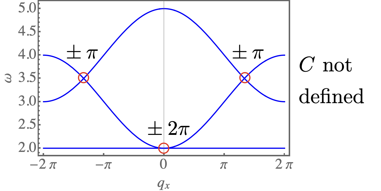
When , magnon bands exhibit a quadratic band–touching points at the zone center , and linear band crossings (Dirac points) at the zone corners . This band structure, illustrated in Fig. S3a and Fig. 3 of the main text, is topologically critical: a Berry phase of is associated with the quadratic band touching, while a Berry phase of is associated with each of the Dirac points. However, these contributions are singular, with the contributions to Berry phase concentrated at the band–touching points. And in the absence of a gap, Chern numbers for the individual bands remain ill–defined.
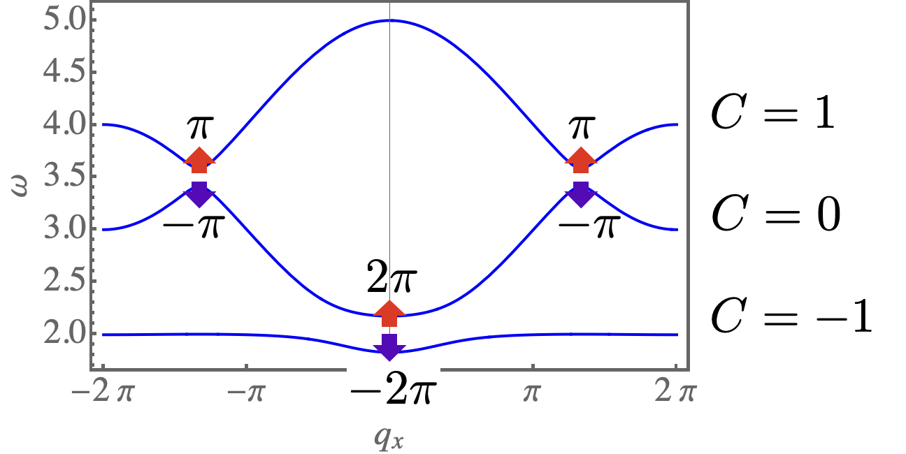
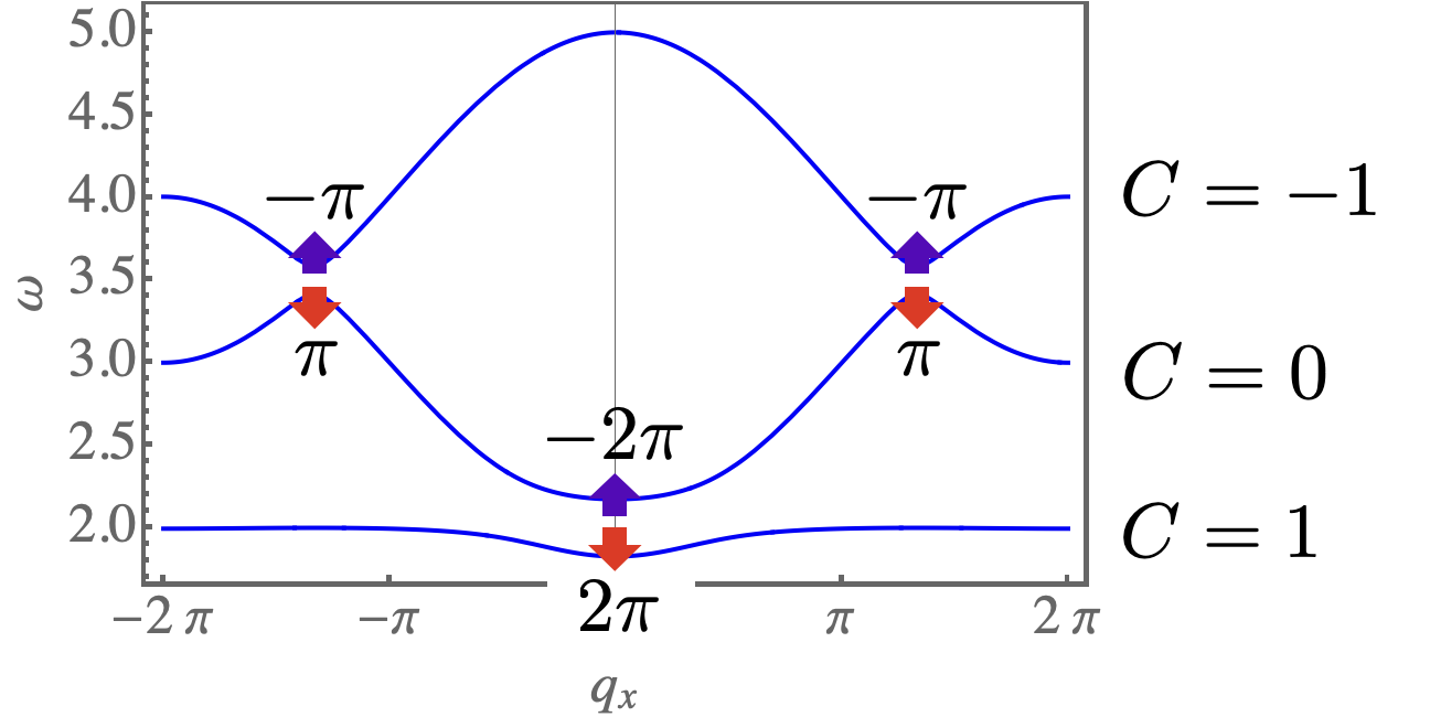
The case with represents a line of critical points of Eq. (S1), for which both and act as singular perturbations. An infinitesimal value of either or is sufficient to open gaps at all three band–touching points, and endow the magnon bands with finite Chern numbers. In the case of finite (), the singular contributions to Berry phase coming from the band–touching points are resolved so as to give Chern numbers , as illustrated in Fig. S3b. This is the case discussed in the main text [cf. Fig. 3 of main text]. Changing the sign of changes the sign of its contributions, without changing their relative phase, leading to Chern numbers . This case is illustrated in Fig. S3c.
The bond–symmetric interaction also mixes states between different bands, opening a gap at all three band–touching points, and leading to a non–trivial band topology. However in this case the relative phase of contributions from quadratic and linear band touchings is reversed, leading to Chern numbers , regardless of the sign of . This case is illustrated in Fig. S3d, and discussed in more detail in Section III.
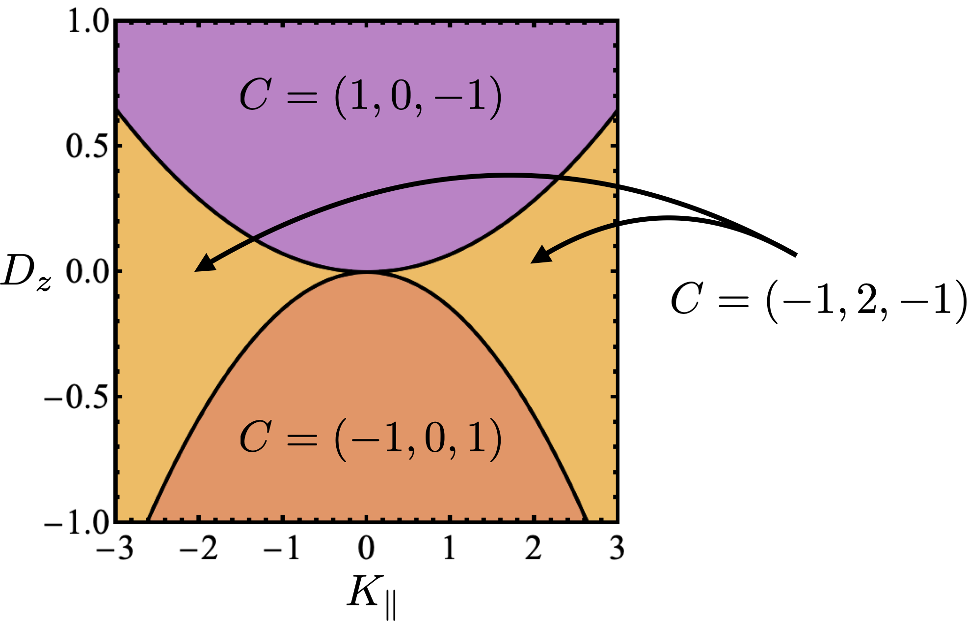
We can derive a general phase diagram for Eq. (S1) as a function of and , by tracking where in parameter space the gaps between bands close. Doing so defines lines in parameter space, where some (or all) of the contributions to Berry curvature coming from band–touching points change sign, leading to a an overall change in Chern numbers. For general , , the gap at the point is given by
| (S37) |
Meanwhile, the gap at the point is
| (S38) |
The two curves defined by
| (S39) |
form the phase boundaries of the phase diagram shown in Fig. S2.
III Role of bond–symmetric anisotropic exchange,
III.1 General considerations
As discussed in Section II.2, the bond–symmetric exchange term, , endows the magnon bands with Chern numbers , in the absence of DM interactions, . The spectral features associated with (avoided) band touching points in this case are qualitatively identical to those discussed for in the main text, and the inferences which can be made about local contributions to Berry phase therefore remain unchanged. However the way in which enters into LSW theory, Eq. (S28), is quite different from .
The DM interactions conserve the number of magnons, and therefore appear in the magnon “hopping” term [Eq. (S20)]. Meanwhile the bond–symmetric exchange term, , introduces magnon–pairing terms, characterised through the matrix [Eq. (S24)]. These pairing terms mix the physical (particle) and unphysical (hole) subspaces of [Eq. (S15)]. Where pairing terms are small compared with the gap between particle and hole subspaces, i.e.
| (S40) |
it is possible to eliminate them from Eq. (S28) by a suitable perturbative canonical transformation [62]. This will have the effect of renormalising magnon hopping term
| (S41) |
and removing from the theory entirely. As a consequence, the form of the equations of motion (EoM) used to describe pinch–point and half–moon features in the main text remain unchanged, along with the conclusions drawn from them about the relationship between spectral features and Berry phase.
In Section III.2 we provide details of the canoncial transformation needed to project pairing terms onto the physical subspace of the LSW theory.
In Section III.3 we derive a general EoM describing an (avoided) quadratic band–touching point in the presence of both and .
III.2 Perturbative canonical transformation
We take as a starting point the Hamiltonian [Eq. (S34)], which determines magnon band structure. The eigenstates of occur with both positive energy (physical subspace) and negative energy (unphysical subspace), and we seek a canonical transformation which will eliminate all terms connecting these two subspaces, such that
| (S44) |
Ideally, this canonical transformation would be carried out exactly as
| (S45) |
where is an appropriate block–off–diagonal matrix. In the absence of prior knowledge of this matrix, we proceed perturbatively, constructing order–by–order in perturbation theory [62].
Since the block-off-diagonal elements in are small compared to the diagonal terms in , Eq. (S40), the unitary transformation must be close to the identity. We can therefore expand the transformation as a power series in
| (S46) |
It follows that the transformed spin-wave Hamiltonian is given by
| (S47) |
with
| (S48) |
As the next step, we separate the block–off–diagonal and block–diagonal parts of . We decouple the spin-wave Hamiltonian as
| (S49) |
here is the block–diagonal part of , containing only matrix elements of [Eq. (S34)]. Within this, contains diagonal elements of , while collects all other block–diagonal terms. Meanwhile, is the block–off–diagonal part of , composed exclusively of matrix elements of and . Under the canonical transformation, Eq. (S48), these terms transform as
| (S50) |
| (S51) |
We are now in a position to solve for by requiring that . Given that the explicit form of the canonical transformation is unknown, we expand as a power series
| (S52) |
where corresponds to the th order of perturbation. We separate the terms of different order in perturbation in . Separating the terms of different orders, we obtain algebraic equations for the matrices
| (S53a) | |||||
| (S53b) | |||||
| (S53c) | |||||
Starting with , we can consecutively solve for the following terms. And using the matrices, we determine
| (S54) |
where denote the th order in perturbation (in this case,
| (S55a) | |||||
| (S55b) | |||||
| (S55c) | |||||
| (S55d) | |||||
Solving (S53a), we find
| (S62) |
Using Eq. (S53b), we can get the second-order correction that includes the effect of the bond–symmetric exchange anisotropy
| (S65) |
where
| (S69) |
This order of perturbation theory is sufficient to capture the effect of on band topology, and we can now work exclusively with the block–diagonal Hamiltonian
| (S72) |
In the limit [Eq. (S40)], this approach exactly reproduces the results of the LSW calculations carried out in the presence of paring terms , as described in Section II, and illustrated in Fig. S1.
III.3 Equation of motion in the long–wavelength limit
Given the block–diagonal Hamiltonian, Eq. (S72), we can derive equations of motions (EoM) for magnon operators of the same form as those given in the main text. We start from the Heisenberg EoM
| (S73) |
where, to accuracy ,
| (S74) |
We now seek expansion of this EoM in the long–wavelength limit (), following the approach described in [53], and outlined in the main text. By so doing, we arrive at a theory of the (avoided) quadratic band touching between the two bands which meet in the zone center.
We start by decoupling Eq. (S74) according to the irreducible representations
| (S75a) | |||||
| (S75b) | |||||
We further use a Helmholtz–Hodge decomposition to separate the two–dimensional irrep. into incompressible and irrotational parts
| (S76) |
satisfying
| (S77) |
These fields obey the coupled EoM
| (S78) | ||||
| (S79) |
where
| (S80) |
It follows directly from Eqs. (S78,S79) that a mixing of incompressible and irrotational excitations occurs whenever the bond–symmetric exchange anisotropy , or DM inteaction, , is finite. As a result, a gap opens at the point whenever either term is non–zero. The continuum theory predicts this gap to be
| (S81) |
This is consistent with the result for found in LSW theory, Eq. S37.
It also follows from Eqs. (S78,S79) that the bond–symmetric interaction has the same effect on excitations near the quadratic band touching as a positive value of DM interaction, , regardless of the sign of . This fact is consistent with the contributions to Chern numbers found in LSW theory [cf. Fig. S3b and Fig. S3d]. And it implies that the result for the dynamical structure factor [Eq. (11) of main text], remains valid as long as appropriately–renormalised values are used for the hydrodynamic parameters and [cf. Eq. (S80)]. Viewed in this light, half moons make no distinction between and . However the presence of magnon–pairing terms coming from would lead to a reduction in the “saturated” moment of system, which might be observable in experiment.
We conclude by noting that the coupled EoM describing the quadratic band–touching can also be solved using Greens functions, within a Nambu (matrix) formalism. In this approach pairing terms can be incorporated directly in EoM, without the need to first project into the physical subspace of the model.