Placement is not Enough: Embedding with Proactive Stream Mapping on the Heterogenous Edge

Hailiang Zhao2, Shuiguang Deng2, Zijie Liu2, Zhengzhe Xiang3, and Jianwei Yin2 2College of Computer Science and Technology, Zhejiang University 3College of Computer Science and Technology, Zhejiang University City College

Abstract

Edge computing is naturally suited to the applications generated by Internet of Things (IoT) nodes. The IoT applications generally take the form of directed acyclic graphs (DAGs), where vertices represent interdependent functions and edges represent data streams. The status quo of minimizing the makespan of the DAG motivates the study on optimal function placement. However, current approaches lose sight of proactively mapping the data streams to the physical links between the heterogenous edge servers, which could affect the makespan of DAGs significantly. To solve this problem, we study both function placement and stream mapping with data splitting simultaneously, and propose the algorithm DPE (Dynamic Programming-based Embedding). DPE is theoretically verified to achieve the global optimality of the embedding problem. The complexity analysis is also provided. Extensive experiments on Alibaba cluster trace dataset show that DPE significantly outperforms two state-of-the-art joint function placement and task scheduling algorithms in makespan by $43.19$ % and $40.71$ %, respectively.

I Introduction

Nowadays, widely used stream processing platforms, such as Apache Spark, Apache Flink, Amazon Kinesis Streams, etc., are designed for large-scale data-centers. These platforms are not suitable for real-time and latency-critical applications running on widely spread Internet of Things (IoT) nodes. By contrast, near-data processing within the network edge is a more applicable way to gain insights, which leads to the birth of edge computing. However, state-of-the-art edgy stream processing systems, for example, Amazon Greengrass, Microsoft Azure IoT Edge and so on, do not consider that how the dependent functions of the IoT applications distributed to the resource-constrained edge. To address this limitation, works studying function placement across the distributed edge servers spring up [1, 2, 3]. In these works, the IoT application is structured as a service function chain (SFC) or a directed acyclic graph (DAG) composed of interdependent functions, and the placement strategy of each function is obtained by minimizing the makespan of the application, under the trade-off between node processing time and cross-node communication overhead.

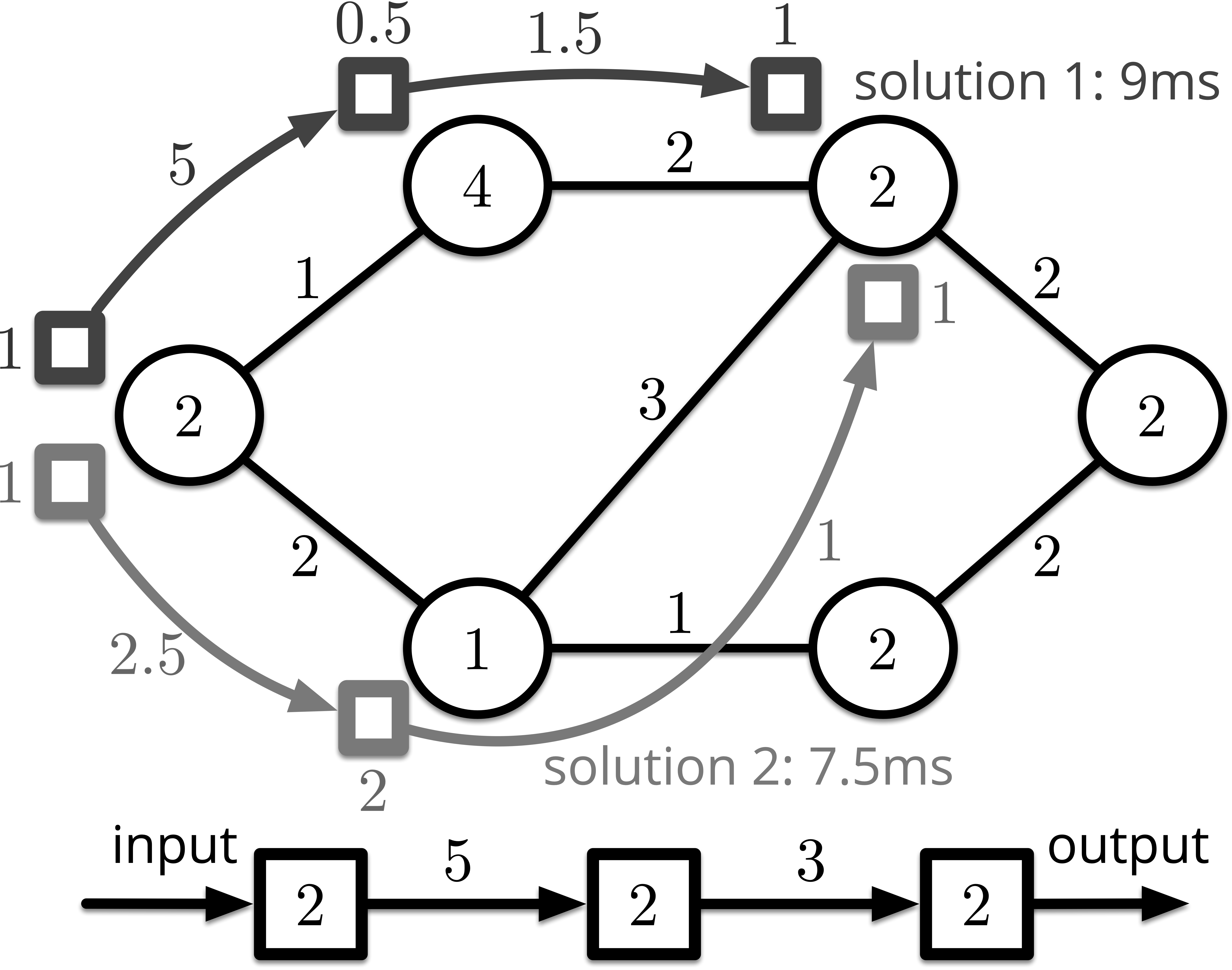
However, when minimizing the makespan of the application, state-of-the-art approaches only optimize the placement of functions, while passively generate the stream mapping. Here the stream mapping refers to mapping the input/output streams to the physical links between edge servers. The passivity here means the routing path between each placed function is not optimized but generated automatically through SDN controllers. Nevertheless, for the heterogenous edge, where each edge server has different processing power and each link has various throughput, better utilization of the stream mapping can result in less makespan even though the corresponding function placement is worse. This phenomenon is illustrated in Fig. 1. The top half of this figure is an undirected connected graph of six edge servers, abstracted from the physical infrastructure of the heterogenous edge. The numbers tagged in each node and beside each link of the undirected graph are the processing power (measured in flop/s) and throughput (measured in bit/s), respectively. The bottom half is a SFC with three functions. The number tagged inside each function is the required processing power (measured in flops). The number tagged beside each data stream is the size of it (measured in bits). Fig. 1 demonstrates two solutions of function placement. The numbers tagged beside nodes and links of each solution are the time consumed (measured in second). Just in terms of function placement, solution 1 enjoys lower function processing time ( $2.5$ s $<$ $4$ s), thus performs better. However, the makespan of solution 2 is $1.5$ s lesser than solution 1 because the path which solution 2 routes through possess a higher throughput.

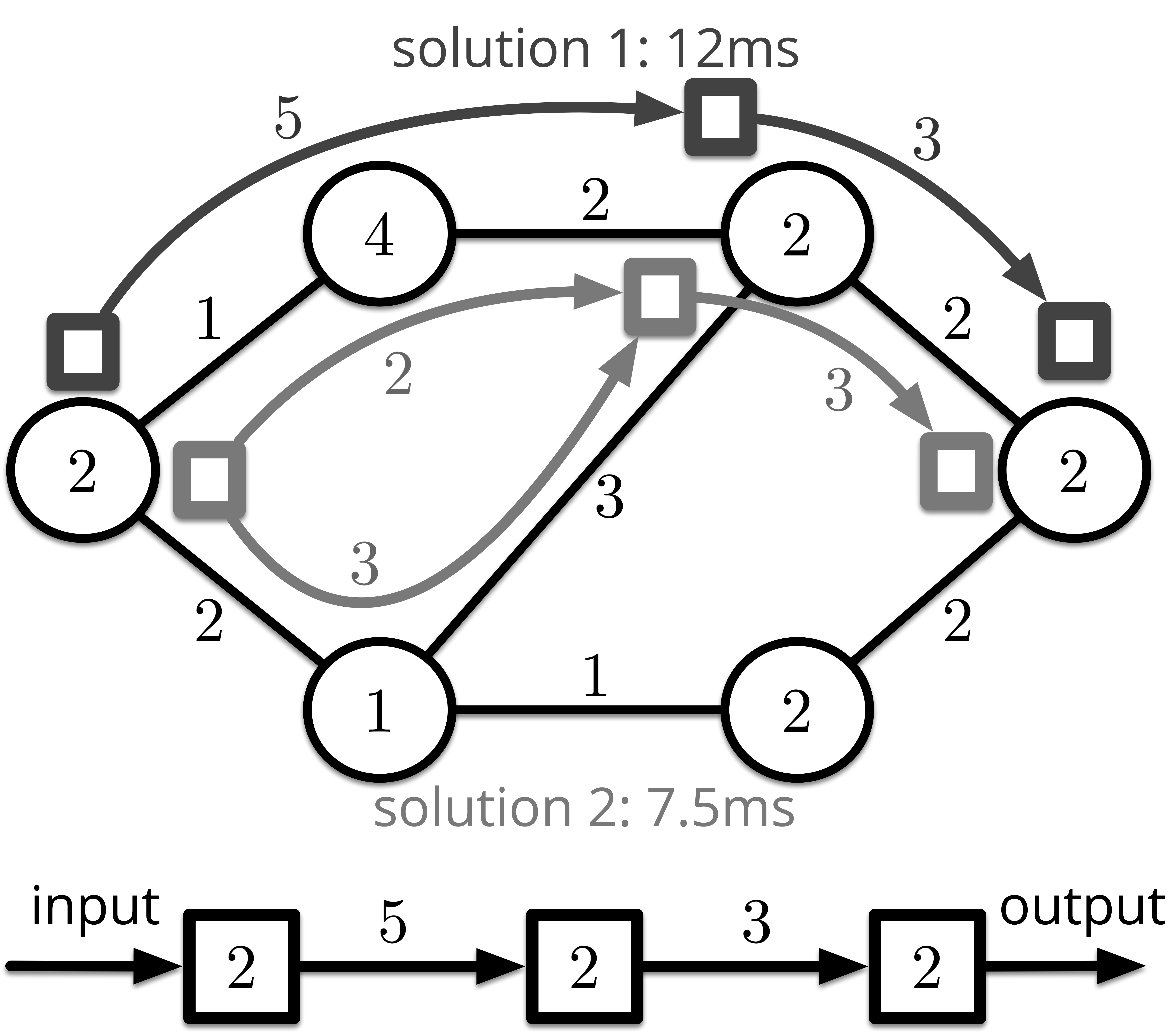
Refer to caption — Figure 1: Two function placement solutions with different stream mappings.

The above example implies that different stream mappings can significantly affect the makespan of the IoT applications. It enlightenes us to take the stream mapping into consideration proactively. In this paper, we name the combination of function placement and stream mapping as function embedding. Moreover, if stream splitting is allowed, i.e., the output data stream of a function can be splitted and route on multiple paths, the makespan can be decreased further. This phenomenon is captured in Fig. 2. The structure of this figure is the same as Fig. 1. It demonstrates two function embedding solutions with stream splitting allowed or not, respectively. In solution 2, the output stream of the first function is divided into two parts, with $2$ bits and $3$ bits, respectively. Correspondingly, the time consumed on routing are $3$ s and $2.5$ s, respectively. Although the two solutions have the same function placement, the makespan of solution 2, which is calculated as $1+\max\{3,2.5\}+1+1.5+1=7.5$ s, is $4.5$ s lesser than solution 1. In practice, segment routing (SR) can be applied to split and route data stream to different edge servers by commercial DNS controllers and HTTP proxies [4].

To capture the importance of stream mapping and embrace the future of 5G communications, in this paper we study the dependent function embedding problem with stream splitting on the heterogenous edge. The problem is similar with Virtual Network Embedding (VNE) problem in 5G network slicing for virtualized network functions (VNFs) [5]. The difference lies in that the VNFs are user planes, management planes and control planes with different levels of granularities, which are virtualized for transport and computing resources of telecommunication networks [6], rather than the IoT applications this paper refers to. For a DAG with complicated structure, the problem is combinatorial and difficult to solve when it scales up. In this paper, we firstly find the optimal substructure of the problem. The basic framework of our algorithm is based on Dynamic Programming. For each substructure, we seperate several linear programming sub-problems and solve them optimally. We do not adopt the regular iteration-based solvers such as simplex method and dual simplex method, but derive the optimal results directly. At length, our paper make the following contributions:

•

Model contribution: We study the dependent function embedding problem on the heterogenous edge. Other than existing works where only function placement is studied, we novelly take proactive stream mapping and data splitting into consideration and leverage dynamic programming as the approach to embed DAGs of IoT applications onto the constrained edge.
•

Algorithm contribution: We present an algorithm that solves the dependent function embedding problem optimally. We firstly find the optimal substructure of the problem. In each substructure, when the placement of each function is fixed, we derive the paths and the data size routes through each path optimally.
•

Experiment contribution: We conduct extensive simulations on a cluster trace with 20365 unique DAGs from Alibaba [7]. Experiment results show that our algorithm significantly outperforms two algorithm, FixDoc [1] and HEFT [8], on the average completion time by $43.19$ % and $40.71$ %, respectively.

The remainder of the paper is organized as follows. In Sec. II, we present the system model and formulate the problem. In Sec. III, we present the proposed algorithms. Performance guarantee and complexity analysis are provided in Sec. IV. The experiment results are demonstrated in Sec. V. In Sec. VI, we review related works on functions placement on the heterogenous edge. Sec. VII concludes this paper.

II System Model

Let us formulate the heterogenous edge as an undirected connected graph $\mathcal{G}\triangleq(\mathcal{N},\mathcal{L})$ , where $\mathcal{N}\triangleq\{n_{1},...,n_{N}\}$ is the set of edge servers and $\mathcal{L}\triangleq\{l_{1},...,l_{L}\}$ is the set of links. Each edge server $n\in\mathcal{N}$ has a processing power $\psi_{n}$ , measured in flop/s while each link $l\in\mathcal{L}$ has the same uplink and downlink throughput $b_{l}$ , measured in bit/s.

II-A Application as a DAG

The IoT application with interdependent functions is modeled as a DAG. The DAG can have arbitrary shape, not just linear SFC. In addition, multi-entry multi-exit is allowed. We write $(\mathcal{F},\mathcal{E})$ for the DAG, where $\mathcal{F}\triangleq\{f_{1},...,f_{Q}\}$ is the set of $Q$ interdependent functions listed in topological order. $\forall f_{i},f_{j}\in\mathcal{F},i\neq j$ , if the output stream of $f_{i}$ is the input of its downstream function $f_{j}$ , a directed link $e_{ij}$ exists. $\mathcal{E}\triangleq\{e_{ij}|\forall f_{i},f_{j}\in\mathcal{F}\}$ is the set of all directed links. For each function $f_{i}\in\mathcal{F}$ , we write $c_{i}$ for the required number of floating point operations of it. For each directed link $e_{ij}\in\mathcal{E}$ , the data stream size is denoted as $s_{ij}$ (measured in bits).

II-B Dependent Function Embedding

We write $p(f_{i})\in\mathcal{N}$ for the chosen edge server which $f_{i}$ to be placed on, and $\mathcal{P}(e_{ij})$ for the set of paths from $p(f_{i})$ to $p(f_{j})$ . Obviously, for all path $\varrho\in\mathcal{P}(e_{ij})$ , it consists of links from $\mathcal{L}$ without duplication. For a function pair $(f_{i},f_{j})$ and its associated directed link $e_{ij}\in\mathcal{E}$ , the data stream can be splitted and route through different paths from $\mathcal{P}(e_{ij})$ . $\forall\varrho\in\mathcal{P}(e_{ij})$ , let us use $z_{\varrho}$ to represent the allocated data stream size for path $\varrho$ . Then, $\forall e_{ij}\in\mathcal{E}$ , we have the following constraint:

\sum_{\varrho\in\mathcal{P}(e_{ij})}z_{\varrho}=s_{ij}.

(1)

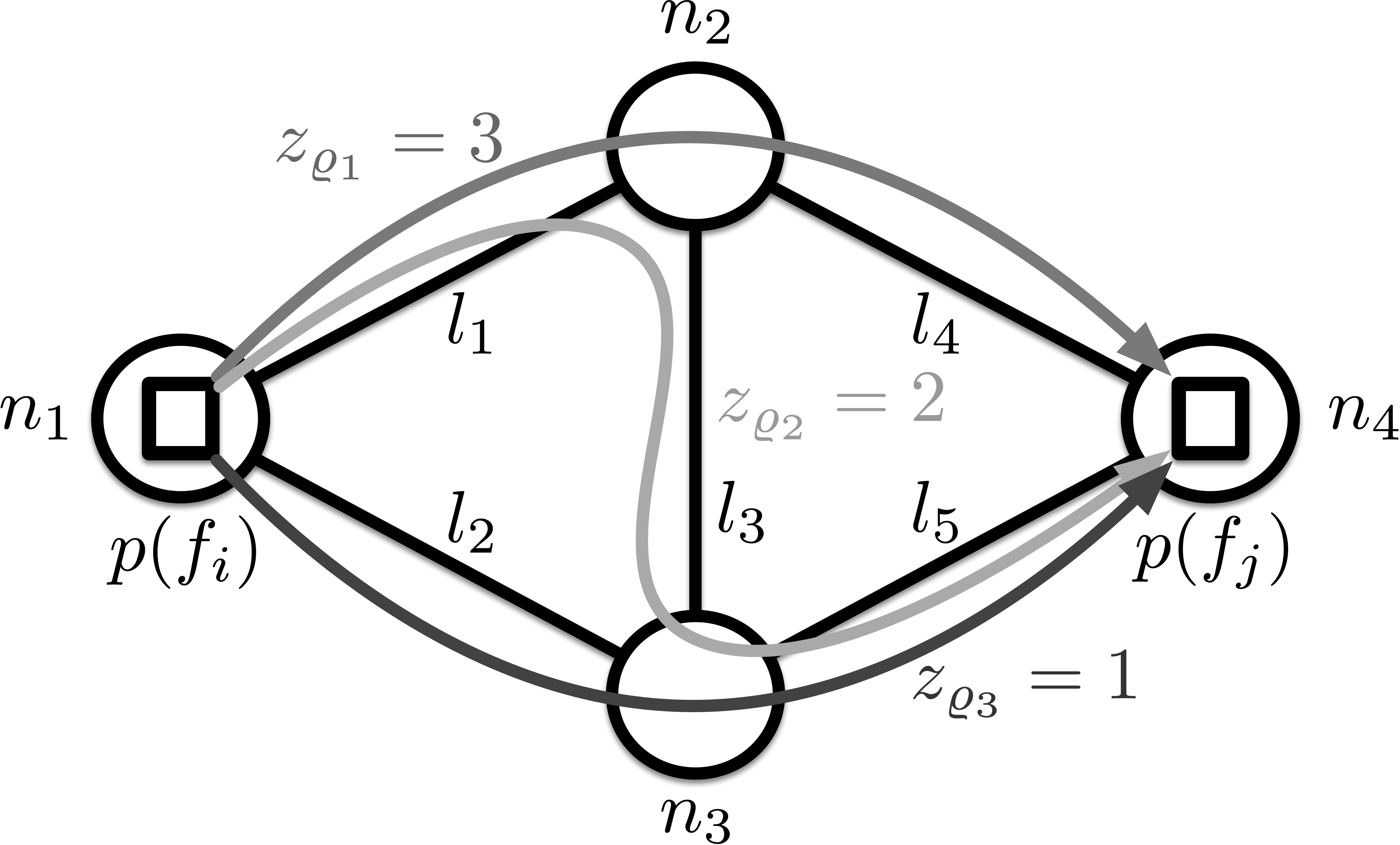
Notice that if $p(f_{i})=p(f_{j})$ , i.e., $f_{i}$ and $f_{j}$ are placed on the same edge server, then $\mathcal{P}(e_{ij})=\varnothing$ and the routing time is zero. Fig. 3 gives a working example. The connected graph in it has four edge servers and five links, from $l_{1}$ to $l_{5}$ . The two squares represents the source function $f_{i}$ and the destination function $f_{j}$ . From the edge server $p(f_{i})$ to the edge server $p(f_{j})$ , $e_{ij}$ routes through three paths with data size of $3$ bits, $2$ bits, and $1$ bits, respectively. In this example, $s_{ij}=6$ . On closer observation, we can find that two data streams route through $l_{1}$ . Each of them is from path $\varrho_{1}$ and $\varrho_{2}$ with $3$ bits and $2$ bits, respectively.

II-C Involution Function of Finish Time

Let us use $T\big{(}p(f_{i})\big{)}$ to denote the finish time of $f_{i}$ on edge server $p(f_{i})$ . Considering that the functions of the DAG have interdependent relations, for each function pair $(f_{i},f_{j})$ where $e_{ij}$ is defined, $T\big{(}p(f_{j})\big{)}$ should involve according to

T\big{(}p(f_{j})\big{)}=\max_{\forall i:e_{ij}\in\mathcal{E}}\Big{(}T\big{(}p(f_{i})\big{)}+t(e_{ij})\Big{)}+t\big{(}p(f_{j})\big{)},

(2)

where $t(e_{ij})$ is the routing time of the directed link $e_{ij}$ and $t\big{(}p(f_{j})\big{)}$ is the processing time of $f_{j}$ on edge server $p(f_{j})$ . Corresponding to (2), for each entry function $f_{i}$ ,

T\big{(}p(f_{i})\big{)}=t\big{(}p(f_{i})\big{)}+rt_{p(f_{i})},

(3)

where $rt_{p(f_{i})}$ stores the beginning time for processing $f_{i}$ . If $f_{i}$ is the first function which is scheduled on server $p(f_{i})$ , $rt_{p(f_{i})}$ is zero. Otherwise, it is the finish time of the last function which is scheduled on server $p(f_{i})$ .

$\forall e_{ij}\in\mathcal{E}$ , $t(e_{ij})$ is decided by the paths in $\mathcal{P}(e_{ij})$ . Specifically, when $f_{i}$ and $f_{j}$ are not placed on the same edge server,

t(e_{ij})=\max_{\varrho\in\mathcal{P}(e_{ij})}\sum_{l\in\varrho}\frac{z_{\varrho}}{b_{l}},

(4)

where $\mathds{1}\{\cdot\}$ is the indicator function. (4) means that the routing time is decided by the slowest branch of data streams. Solution 2 in Fig. 2 is an example.

$\forall f_{j}\in\mathcal{F}$ , $t\big{(}p(f_{j})\big{)}$ is decided by the processing power of the chosen edge server $p(f_{j})$ :

t\big{(}p(f_{j})\big{)}=\frac{c_{j}}{\psi_{p(f_{j})}}.

(5)

To describe the earliest makespan of the DAG, inspired by [1], we add a dummy tail function $f_{Q+1}$ . As a dummy function, the processing time of $f_{Q+1}$ is set as zero whichever edge server it is placed on. That is,

t\big{(}p(f_{Q+1})\big{)}=0,\forall p(f_{Q+1})\in\mathcal{N}.

(6)

Besides, each destination function needs to point to $f_{Q+1}$ with a link weight of its output data stream size. We write $\mathcal{F}_{dst}\subset\mathcal{F}$ for the set of destination functions and $\mathcal{F}_{src}$ for the set of entry functions of the DAG. In addition, we write $\mathcal{E}_{dmy}$ for the set of new added links which point to $f_{Q+1}$ , i.e.,

\mathcal{E}_{dmy}\triangleq\{e_{i,Q+1}|\forall f_{i}\in\mathcal{F}_{dst}\}.

(7)

As such, the DAG is updated as $(\mathcal{F}^{\prime},\mathcal{E}^{\prime})$ , where $\mathcal{F}^{\prime}\triangleq\mathcal{F}\cup\{f_{Q+1}\}$ and $\mathcal{E}^{\prime}\triangleq\mathcal{E}\cup\mathcal{E}_{dmy}$ .

II-D Problem Formulation

Our target is to minimize the makespan of the DAG by finding the optimal $p(f_{i})$ , $\mathcal{P}(e_{ij})$ , and $z_{\varrho}$ for all $f_{i}\in\mathcal{F}^{\prime}$ , $e_{ij}\in\mathcal{E}^{\prime}$ , and $\varrho\in\mathcal{P}(e_{ij})$ . Let us use $T^{\star}\big{(}p(f_{i})\big{)}$ to represent the earliest finish time of $f_{i}$ on edge server $p(f_{i})$ . Further, we use $T\big{(}\mathcal{F}^{\prime},\mathcal{E}^{\prime},p(f_{Q+1})\big{)}$ to represent the earliest makespan of the DAG when $f_{Q+1}$ is placed on $p(f_{Q+1})$ . Obviously, it is equal to $T^{\star}\big{(}p(f_{Q+1})\big{)}$ . The dependent function embedding problem can be formulated as:

	$\displaystyle\mathbf{P}:\min_{\forall p(f_{i}),\forall\mathcal{P}(e_{ij}),\forall z_{\varrho}}T\Big{(}\mathcal{F}^{\prime},\mathcal{E}^{\prime},p(f_{Q+1})\Big{)}$
	$\displaystyle s.t.\qquad\qquad\qquad\eqref{cons1},\qquad\qquad\qquad$
	$\displaystyle\quad z_{\varrho}\geq 0,\forall\varrho\in\mathcal{P}(e_{ij}),\forall e_{ij}\in\mathcal{E}^{\prime}.$		(8)

III Algorithm Design

III-A Finding Optimal Substructure

The set of function embedding problems are proved to be NP-hard [5]. As a special case of these problems, $\mathbf{P}$ is NP-hard, too. because of the dependency relations of fore-and-aft functions, the optimal placement of functions and optimal mapping of data streams cannot be obtained simultaneously. Nevertheless, we can solve it by finding its optimal substructure.

Let us dig deeper into the involution equation (2). We can find that

T\big{(}p(f_{j})\big{)}=\max_{\forall i:e_{ij}\in\mathcal{E}^{\prime}}\Big{(}T\big{(}p(f_{i})\big{)}+t(e_{ij})+t\big{(}p(f_{j})\big{)}\Big{)}

(9)

because $t\big{(}p(f_{j})\big{)}$ has no impact on $\max_{\forall i:e_{ij}\in\mathcal{E}^{\prime}}(\cdot)$ . Notice that $\mathcal{E}$ is replaced by $\mathcal{E}^{\prime}$ . Then the following expression holds:

	$\displaystyle\quad T^{\star}\big{(}p(f_{j})\big{)}=\max_{\forall i:e_{ij}\in\mathcal{E}^{\prime}}\Big{\{}\min_{p(f_{i}),\mathcal{P}(e_{ij}),z_{\varrho}}$
	$\displaystyle\quad\Big{(}T^{\star}\big{(}p(f_{i})\big{)}+t(e_{ij})+t\big{(}p(f_{j})\big{)}\Big{)}\Big{\}}.$		(10)

Besides, for all the entry functions $f_{i}\in\mathcal{F}_{src}$ , $T^{\star}\big{(}p(f_{i})\big{)}$ is calculated by (3) without change.

With (10), for each function pair $(f_{i},f_{j})$ where $e_{ij}$ exists, we define the sub-problem $\mathbf{P}_{sub}$ :

	$\displaystyle\mathbf{P}_{sub}:\min_{p(f_{i}),\mathcal{P}(e_{ij}),z_{\varrho}}\mathbf{\Phi}_{ij}\triangleq T^{\star}\big{(}p(f_{i})\big{)}+t(e_{ij})+t\big{(}p(f_{j})\big{)}$
	$\displaystyle s.t.\quad\eqref{cons1},\eqref{cons2}.\qquad\qquad\qquad\qquad\qquad$

In $\mathbf{P}_{sub}$ , $p(f_{j})$ is fixed. We need to decide where $f_{i}$ shoud be placed and how $e_{ij}$ is mapped. Based on that, $T^{\star}\big{(}p(f_{j})\big{)}$ can be updated by $\max_{\forall i:e_{ij}\in\mathcal{E}^{\prime}}\min_{p(f_{i}),\mathcal{P}(e_{ij}),z_{\varrho}}\mathbf{\Phi}_{ij}$ . As a result, $\mathbf{P}$ can be solved optimally by calculating the earliest finish time of each function in turn.

The analysis is captured in Algorithm 1, i.e. Dynamic Programming-based Embedding (DPE). Firstly, DPE finds all the simple paths (paths without loops) between any two edge servers $n_{i}$ and $n_{j}$ , i.e. $\mathcal{P}(e_{ij})$ (Step 2 $\sim$ Step 6). It will be used to calculate the optimal $z_{\varrho}^{\star}$ and $\mathcal{P}^{\star}(e_{ij})$ . For all the functions $f_{i}$ who directly point to $f_{j}$ , DPE firstly fixs the placement of $f_{j}\in\mathcal{N}$ . Then, for the function pair $(f_{i},f_{j})$ , $\mathbf{P}_{sub}$ is solved and the optimal solution is stored in $\mathbf{\Theta}$ (Step 18 $\sim$ Step 19). If $p^{\star}(f_{i})$ has been decided beforehand, $\mathbf{\Phi}^{\star}_{ij}$ can be directly obtained by finding $\mathcal{P}^{\star}(e_{ij})$ and $z^{\star}_{\varrho}$ between $p^{\star}(f_{i})$ and $n$ . The optimal transmission cost is stored in $t^{\star}(e_{ij})$ (Step 11 $\sim$ Step 14). The if statement holds for $f_{i}\in\mathcal{F}^{\prime}$ when $f_{i}$ is a predecessor of multiple functions. Step 12 is actually a sub-problem of $\mathbf{P}_{sub}$ with $p^{\star}(f_{i})$ fixed. Notice that the calculation of the finish time of the entry functions and the other functions are different (Step 16 and Step 21, respectively). At last, the global minimal makespan of the DAG is $\min_{p_{(}f_{Q+1})}T^{\star}(p(f_{Q+1}))$ . The optimal embedding of each function can be retrieved from $\mathbf{\Theta}$ .

Input:

\mathcal{G}

and

(\mathcal{F}^{\prime},\mathcal{E}^{\prime})

Output: Optimal value and corresponding solution

\mathbf{\Theta}\leftarrow\varnothing

2 for each $n_{i}\in\mathcal{M}$ do

3 for each $n_{j}\in\mathcal{M}\wedge n_{j}\neq n_{i}$ do

4 Find all the simple paths between

n_{i}

and

n_{j}

6 end for

8 end for

9for $j=|\mathcal{F}_{src}|+1$ to $Q+1$ do

10 for each $n\in\mathcal{N}$ do

p(f_{j})\leftarrow n

// Fix the placement of

f_{j}

12 for each $f_{i}\in\{f_{i}|e_{ij}\textrm{ exists}\}$ do

13 if $p^{\star}(f_{i})$ has been decided then

\mathbf{\Phi}^{\star}_{ij}\leftarrow T^{\star}\big{(}p^{\star}(f_{i})\big{)}+t^{\star}(e_{ij})+t\big{(}p(f_{j})\big{)}

15 goto Step 19

17 end if

18 if $f_{i}\in\mathcal{F}_{src}$ then

\forall p(f_{i})\in\mathcal{N}

, update

T^{\star}\big{(}p(f_{i})\big{)}

by (3)

21 end if

22 Obtain the optimal

\mathbf{\Phi}^{\star}_{ij}

p^{\star}(f_{i})

\mathcal{P}^{\star}(e_{ij})

, and

z^{\star}_{\varrho}

by solving

\mathbf{P}_{sub}

\boldsymbol{\Theta}.append\Big{(}\big{\{}p^{\star}(f_{i})\big{\}}\times\big{\{}\mathcal{P}^{\star}(e_{ij})\big{\}}\times\big{\{}z^{\star}_{\varrho}|\forall\varrho\in\mathcal{P}^{\star}(e_{ij})\big{\}}\Big{)}

25 end for

26 Update

T^{\star}\big{(}p(f_{j})\big{)}

by (10)

28 end for

30 end for

return $\min_{p_{(}f_{Q+1})}T^{\star}(p(f_{Q+1}))$ and $\mathbf{\Theta}$

Algorithm 1 DP-based Embedding (DPE)

III-B Optimal Proactive Stream Mapping

Now the problem lies in that how to find all the simple paths and solve $\mathbf{P}_{sub}$ optimally. For the former, we propose a Recursion-based Path Finding (RPF) algorithm, which will be detailed in Sec. III-B1. For the latter, When $p(f_{j})$ is fixed, the value of $t\big{(}p(f_{j})\big{)}$ is known and can be viewed as a constant for $\mathbf{P}_{sub}$ . Besides, from Step 12 of DPE we can find that, for all $f_{i}\in\{f_{i}\in\mathcal{F}^{\prime}-\mathcal{F}_{src}|e_{ij}\textrm{ exists}\}$ , $\forall p(f_{i})\in\mathcal{N}$ , $T^{\star}\big{(}p(f_{i})\big{)}$ is already updated in the last iteration. Thus, for solving $\mathbf{P}_{sub}$ , the difficulty lies in that how to select the optimal placement of $f_{i}$ and the optimal mapping of $e_{ij}$ . It will be detailed in Sec. III-B2.

III-B1 Recursion-based Path Finding

We use $\mathcal{P}(n_{i},n_{j},\mathcal{M})$ to represent the set of simple paths from $n_{i}$ to $n_{j}$ where no path goes through nodes from the set $\mathcal{M}\subseteq\mathcal{N}$ . The set of simple paths from $n_{i}$ to $n_{j}$ we want, i.e. $\mathcal{P}(e_{ij})$ , is equal to $\mathcal{P}(n_{i},n_{j},\varnothing)$ . $\forall n\in\mathcal{N}$ , let us use $\mathcal{A}(n)$ to represent the set of edge servers adjcent to $n$ . Then, $\mathcal{P}(n_{i},n_{j},\mathcal{M})$ can be calculated by the following recursion formula:

\mathcal{P}(n_{i},n_{j},\mathcal{M})=\Big{\{}J(\varrho,n_{i})\Big{|}\bigcup_{m\in\mathcal{S}}\mathcal{P}\big{(}m,n_{j},\mathcal{M}\cup\{n_{i}\}\big{)}\Big{\}},

where $\mathcal{S}\triangleq\mathcal{A}(n_{i})-\mathcal{M}\cup\{n_{i}\}$ . $J(\varrho,n_{i})$ is a function that joins the node $n_{i}$ to the path $\varrho$ and returns the new joint path $\varrho\cup\{n_{i}\}$ . The analysis in this paragraph is summarized in Algorithm 2, i.e. Recursion-based Path Finding (RPF) algorithm.

Before calling RPF, we need to initialize the global variables. Specifically, $\mathbf{\Omega}$ stores all the simple paths, which is initialized as $\varnothing$ . $\mathcal{V}$ , as the set of visited nodes, is initialized as $\varnothing$ . $\varrho$ is allocated for the storage of current path, which is also initialized as $\varnothing$ . Whereafter, by calling $\texttt{RPF}(n_{i},n_{i},n_{j})$ , all the simple paths between $n_{i}$ and $n_{j}$ are stored in $\mathbf{\Omega}$ . $\texttt{RPF}(n_{i},n_{i},n_{j})$ is used to replace Step 4 of DPE.

Input:

n_{i}

n

, and

n_{j}\in\mathcal{N}

1 /* Global variables

n_{i},n_{j},\mathcal{V},\varrho,\mathcal{G},

and

\mathbf{\Omega}

can be visited by RPF. Before calling it,

\mathcal{V}

\varrho

, and

\mathbf{\Omega}

are set as

\varnothing

. */

2 if $n==n_{j}$ then

\mathbf{\Omega}.append\big{(}J(\varrho,n)\big{)}

// Store the path

J(\varrho,n)

5 else

\varrho.push(n)

;

\mathcal{V}.add(n)

7 for each $n^{\prime}\in\mathcal{A}(n)-\mathcal{V}$ do

\texttt{RPF}(n_{i},n^{\prime},n_{j})

// Recursive call

10 end for

\varrho.pop()

;

\mathcal{V}.delete(n)

13 end if

Algorithm 2 Recursion-based Path Finding (RPF)

In the following, we calculate the optimal value of $z_{\varrho}$ for each simple path $\varrho\in\mathbf{\Omega}$ .

III-B2 Optimal Data Splitting

Since both $p(f_{i})$ and $p(f_{j})$ are fixed, $T^{\star}\big{(}p(f_{i})\big{)}$ and $t\big{(}p(f_{i})\big{)}$ are constants. Therefore, solving $\mathbf{P}_{sub}$ is equal to solving the following problem:

	$\displaystyle\mathbf{P}^{\prime}_{sub}:$	$\displaystyle\min_{\forall\varrho\in\mathbf{\Omega}:z_{\varrho}}\max_{\varrho\in\mathbf{\Omega}}\bigg{\{}\Big{(}\sum_{l\in\varrho}\frac{1}{b_{l}}\Big{)}\cdot z_{\varrho}\bigg{\}}$			(13)
		$\displaystyle s.t.\quad\left\{\begin{array}[]{c}\sum_{\varrho\in\mathbf{\Omega}}z_{\varrho}=s_{ij},\\ z_{\varrho}\geq 0,\forall\varrho\in\mathbf{\Omega}.\end{array}\right.\qquad\qquad$			(13)

(13) is reconstructed from (1) and (8). To solve $\mathbf{P}^{\prime}_{sub}$ , we define a diagonal matrix

\mathbf{A}\triangleq\operatorname*{diag}\bigg{(}\sum_{l_{1}\in\varrho_{1}}\frac{1}{b_{l_{1}}},\sum_{l_{2}\in\varrho_{2}}\frac{1}{b_{l_{2}}},...,\sum_{l_{|\mathbf{\Omega}|}\in\varrho_{|\mathbf{\Omega}|}}\frac{1}{b_{l_{|\mathbf{\Omega}|}}}\bigg{)}.

Obviously, all the diagonal elements of $\mathbf{A}$ are positive real numbers. The variables that need to be determined can be written as $\mathbf{z}\triangleq[z_{\varrho_{1}},z_{\varrho_{2}},...,z_{\varrho_{|\mathbf{\Omega}|}}]^{\top}\in\mathbb{R}^{|\mathbf{\Omega}|}$ . Thus, $\mathbf{P}^{\prime}_{sub}$ can be transformed into

	$\displaystyle\mathbf{P}_{norm}:$	$\displaystyle\min_{\mathbf{z}}\\|\mathbf{A}\mathbf{z}\\|_{\infty}\qquad\quad$
	$\displaystyle s.t.$	$\displaystyle\left\{\begin{array}[]{c}\mathbf{1}^{\top}\mathbf{z}=s_{ij},\\ \mathbf{z}\geq\mathbf{0}.\end{array}\right.\qquad\quad$			(16)

$\mathbf{P}_{norm}$ is an infinity norm minimization problem. By introducing slack variables $\tau\in\mathbb{R}$ and $\mathbf{y}\in\mathbb{R}^{|\mathbf{\Omega}|}$ , $\mathbf{P}_{norm}$ can be transformed into the following linear programming problem:

	$\displaystyle\mathbf{P}^{\prime}_{norm}:\min_{\mathbf{z}^{\prime}\triangleq[\mathbf{z}^{\top},\mathbf{y}^{\top}]^{\top}}\tau\qquad$
	$\displaystyle s.t.\quad\left\{\begin{array}[]{c}\sum_{\varrho\in\mathbf{\Omega}}z_{\varrho}=s_{ij},\\ \mathbf{A}\mathbf{z}+\mathbf{y}=\tau\cdot\mathbf{1},\\ \mathbf{z}^{\prime}\geq\mathbf{0}.\end{array}\right.$

$\mathbf{P}^{\prime}_{norm}$ is feasible and its optimal objective value is finite. As a result, simplex method and dual simplex method can be applied to obtain the optimal solution efficiently.

However, simplex methods might be time-consuming when the scale of $\mathcal{G}$ increases. In fact, we can find that the optimal objective value of $\mathbf{P}_{norm}$ is

\min_{\mathbf{z}}\|\mathbf{A}\mathbf{z}\|_{\infty}=\frac{s_{ij}}{\sum_{k=1}^{|\mathbf{\Omega}|}1/A_{k,k}},

(18)

if and only if

A_{u,u}\mathbf{z}^{(u)}=A_{v,v}\mathbf{z}^{(v)},1\leq u\neq v\leq|\mathbf{\Omega}|,

(19)

where $\mathbf{z}^{(u)}$ is the $u$ -th component of vector $\mathbf{z}$ and $A_{u,u}$ is the $u$ -th diagonal element of $\mathbf{A}$ . Detailed proof of this result is provided in Sec. IV-A. Base on (19), we can infer that the optimal variable $\mathbf{z}^{\star}>\mathbf{0}$ , which means that $\forall\varrho\in\mathbf{\Omega}$ , $z^{\star}_{\varrho}\neq 0$ . Therefore, the assumption in Sec. III-B1 is not violated and the optimal $\mathcal{P}^{\star}(e_{ij})$ is equivalent to $\mathbf{\Omega}$ .

Input:

\mathcal{G}

(\mathcal{F}^{\prime},\mathcal{E}^{\prime})

, and

p(f_{j})

Output: The optimal

\mathbf{\Phi}^{\star}_{ij}

p^{\star}(f_{i})

\mathcal{P}^{\star}(e_{ij})

, and

\mathbf{z}^{\star}

1 for each $m\in\mathcal{N}$ do in parallel

p(f_{i})\leftarrow m

3 /* Obtain the

m

-th optimal

\mathbf{\Phi}_{ij}

by (18) */

\mathbf{\Phi}_{ij}^{(m)}\leftarrow\frac{s_{ij}}{\sum_{k}1/A_{k,k}^{(m)}}+T^{\star}\big{(}p(f_{i})\big{)}+t\big{(}p(f_{j})\big{)}

6 end for

p^{\star}(f_{i})\leftarrow\operatorname*{argmin}_{m\in\mathcal{N}}\boldsymbol{\Phi}_{ij}^{(m)}

\mathcal{P}^{\star}(e_{ij})\leftarrow\mathbf{\Omega}^{(p^{\star}(f_{i}))}

9 Calculate

\mathbf{z}^{\star}

by (16) and (19) with

\mathbf{A}=\mathbf{A}^{(p^{\star}(f_{i}))}

return $\mathbf{\Phi}^{(p^{\star}(f_{i}))}_{ij}$ , $p^{\star}(f_{i})$ , $\mathcal{P}^{\star}(e_{ij})$ , and $\mathbf{z}^{\star}$

Algorithm 3 Optimal Stream Mapping (OSM)

Up to now, when $p(f_{i})$ is fixed, we have calculate the optimal $\mathcal{P}^{\star}(e_{ij})$ and $z^{\star}_{\varrho}$ for all paths $\varrho\in\mathcal{P}^{\star}(e_{ij})$ . The analysis in this subsection are summarized in Algorithm 3, Optimal Stream Mapping (OSM) algorithm. In OSM, $\mathbf{\Phi}_{ij}^{(m)}$ is the $m$ -th objective value of $\mathbf{P}_{sub}$ by taking $p(f_{i})=m$ . Similarly, $\mathbf{\Omega}^{(p^{\star}(f_{i}))}$ is the $p^{\star}(f_{i})$ -th set of simple paths obtained by RPF. For at most $|\mathcal{N}_{i}|$ choices of $p(f_{i})$ , OSM calculates the optimal objective value (Step 1 $\sim$ Step 5). The procedure is executed in parallel (with different threads) because intercoupling is nonexistent. Then, OSM finds the best placement of $f_{i}$ and returns the corresponding $\mathcal{P}^{\star}(e_{ij})$ , $\mathbf{z}^{\star}$ . OSM is used to replace Step 18 of DPE.

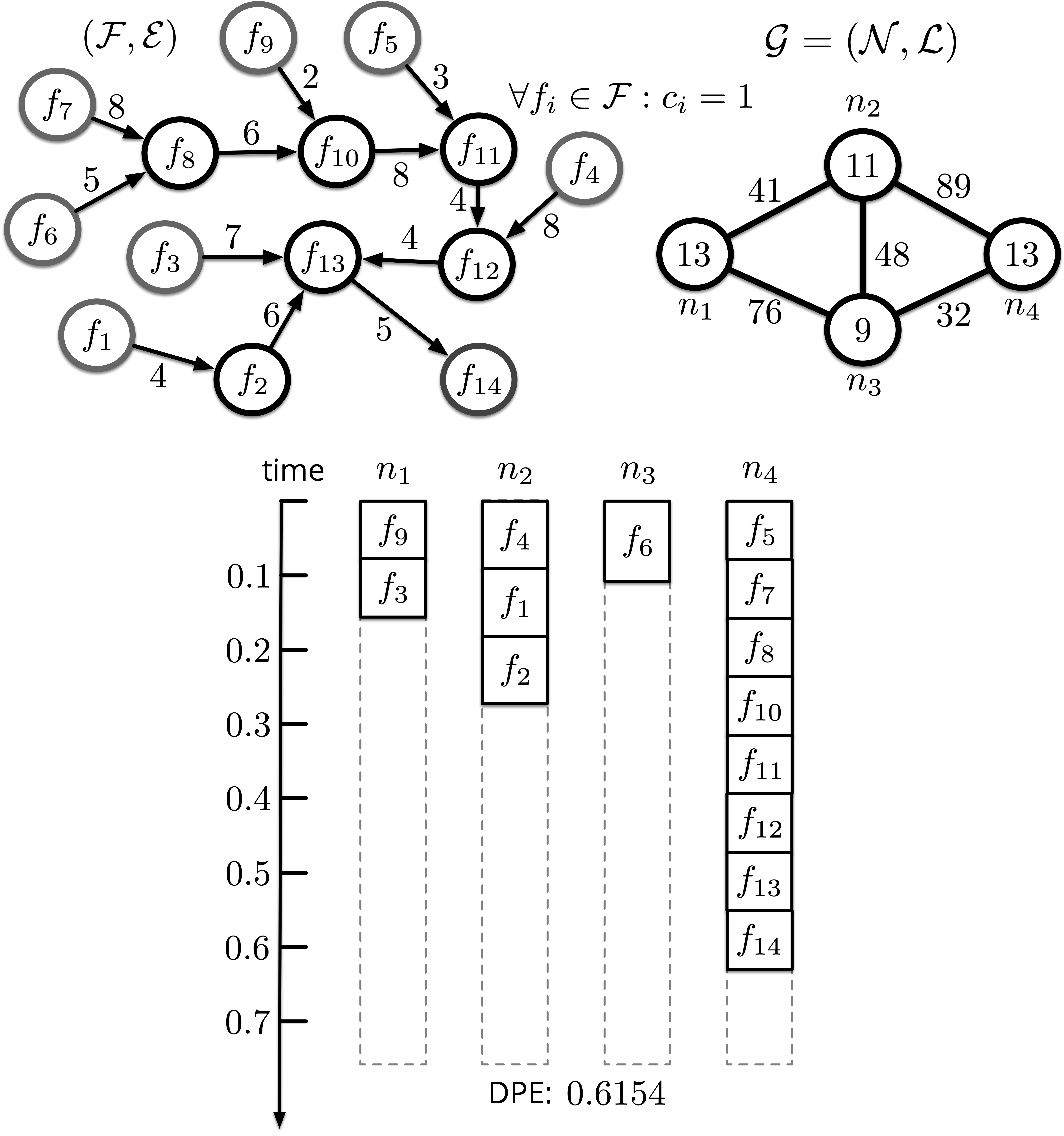
Fig. 4 demonstrates an example on how PDE works. The top left portion of the figure is a DAG randomly sampled from the Alibaba cluster trace, where all the functions are named in the manner of topological order. $\forall f_{i}\in\mathcal{F}$ , $c_{i}$ is set as $1$ . The top right is the edge server cluster $\mathcal{G}$ . The bottom demonstrates how the functions are placed and scheduled by DPE.

IV Theoretical Analysis

IV-A Performance Guarantee

In this subsection, we analyze the optimality of the proposed algorithm, DPE.

Theorem 1.

Optimality of DPE For a DAG $(\mathcal{F},\mathcal{E})$ with a given topological order, DPE can achieve the global optimality of $\mathbf{P}$ by replacing the Step 4 of it with RPF and Step 18 of it with OSM.

Proof.

We firstly prove that OSM solves $\mathbf{P}_{sub}$ optimally. Recall that solving $\mathcal{P}_{sub}$ is equal to solving $\mathbf{P}^{\prime}_{sub}$ , and $\mathbf{P}^{\prime}_{sub}$ can be transformed into $\mathbf{P}_{norm}$ . For $\mathbf{P}_{norm}$ , we have

\|\mathbf{A}\mathbf{z}\|_{\infty}\triangleq\max_{k}\big{\{}|A_{k,k}\mathbf{z}^{(k)}|\big{\}}=\lim_{x\to\infty}\sqrt[x]{\sum_{k=1}^{|\mathbf{\Omega}|}(A_{k,k}\mathbf{z}^{(k)})^{x}}

because $\forall k,A_{k,k}>0,\mathbf{z}^{(k)}\geq 0$ . According to the AM–GM inequality, the following inequality always holds:

\frac{\sum_{k=1}^{|\mathbf{\Omega}|}(A_{k,k}\mathbf{z}^{(k)})^{x}}{|\mathbf{\Omega}|}\geq\sqrt[|\mathbf{\Omega}|]{\prod_{k=1}^{|\mathbf{\Omega}|}(A_{k,k}\mathbf{z}^{(k)})^{x}},

(20)

iff (19) is satisfied. It yields that $\forall x>0$ ,

\displaystyle\sqrt[x]{\frac{\sum_{k=1}^{|\mathbf{\Omega}|}(A_{k,k}\mathbf{z}^{(k)})^{x}}{|\mathbf{\Omega}|}}\geq\sqrt[|\mathbf{\Omega}|]{\prod_{k=1}^{|\mathbf{\Omega}|}A_{k,k}\mathbf{z}^{(k)}}.

(21)

Multiply both sides of (21) by $\sqrt[x]{|\mathbf{\Omega}|}$ , we have

\sqrt[x]{\sum_{k=1}^{|\mathbf{\Omega}|}(A_{k,k}\mathbf{z}^{(k)})^{x}}\geq\sqrt[x]{|\mathbf{\Omega}|}\cdot\sqrt[|\mathbf{\Omega}|]{\prod_{k=1}^{|\mathbf{\Omega}|}A_{k,k}\mathbf{z}^{(k)}}.

(22)

By taking the limit of (22), we have

\|\mathbf{A}\mathbf{z}\|_{\infty}\geq\lim_{x\to\infty}\sqrt[x]{|\mathbf{\Omega}|}\cdot\sqrt[|\mathbf{\Omega}|]{\prod_{k=1}^{|\mathbf{\Omega}|}A_{k,k}\mathbf{z}^{(k)}}.

(23)

Combining with (16) and (19), the right side of (23) is actually a constant. In other words,

$\displaystyle\min_{\mathbf{z}}\\|\mathbf{A}\mathbf{z}\\|_{\infty}$	$\displaystyle=$	$\displaystyle\lim_{x\to\infty}\sqrt[x]{\|\mathbf{\Omega}\|}\cdot\sqrt[\|\mathbf{\Omega}\|]{\prod_{k=1}^{\|\mathbf{\Omega}\|}A_{k,k}\mathbf{z}^{(k)}}$
	$\displaystyle=$	$\displaystyle\sqrt[\|\mathbf{\Omega}\|]{\prod_{k=1}^{\|\mathbf{\Omega}\|}A_{k,k}\mathbf{z}^{(k)}}\quad\rhd\textrm{with \eqref{P_map_cons}}$
	$\displaystyle=$	$\displaystyle\frac{s_{ij}}{\sum_{k=1}^{\|\mathbf{\Omega}\|}1/A_{k,k}}.$

The result shows that (18) and (19) are the optimal objective value and corresponding optimal condition of $\mathbf{P}_{sub}$ , respectively, if the topological ordering is given and regarded as an known variable. The theorem is immediate from the optimality of DP. ∎

IV-B Complexity Analysis

In this subsection, we analyze the complexity of the proposed algorithms in the worst case, where $\mathcal{G}$ is fully connected.

IV-B1 Complexity of RPF

Let us use $\kappa(i,j)$ to denote the flops required to compute all the simple paths between $n_{i}$ and $n_{j}$ . If $\mathcal{G}$ is fully connected,

$\displaystyle\kappa(1,N)$	$\displaystyle=$	$\displaystyle\big{(}1+\kappa(2,N)\big{)}+\big{(}1+\kappa(3,N)\big{)}$
	$\displaystyle+$	$\displaystyle...+\big{(}1+\kappa(N-1,N)\big{)}+1$
	$\displaystyle=$	$\displaystyle(N-1)+(N-2)\cdot\kappa(2,N).$

To simplify notations, we use $\kappa_{i}$ to replace $\kappa(i,N)$ . We can conclude that $\forall i\in\{1,...,N-1\}$ ,

\displaystyle\kappa_{i}=(N-i)+(N-i-1)\cdot\kappa_{i+1}.

(24)

Based on (24), we have

	$\displaystyle\kappa_{1}$	$\displaystyle=$	$\displaystyle(N-2)!\cdot\sum_{i=1}^{N-1}\frac{N-i}{(N-i-1)!}$		(25)
		$\displaystyle=$	$\displaystyle(N-2)!\cdot\sum_{i=1}^{N-1}\frac{i^{2}}{i!}$		(25)

which is the maximum flops required to compute all the simple paths between any two edge servers. Before calculating the complexity of RPF, we prove two lemmas.

Lemma 1.

$\forall N\geq 7$ and $N\in\mathbb{N}^{+}$ , $N!>N^{3}(N+1)$ .

Proof.

The proof is based on induction. When $N=7$ , $N!=5040>N^{3}(N+1)=2744$ . The lemma holds. Assume that the lemma holds for $N=q$ , i.e., $q!>q^{3}(q+1)$ (induction hypothesis). Then, for $N=q+1$ , we have

(q+1)!=(q+1)\cdot q!>(q+1)^{2}q^{3}.

(26)

Notice that the function $g(q)\triangleq(\frac{1}{q}+\frac{2}{q^{2}}+\frac{4}{q^{3}})^{-1}$ monotonically increases when $q\in\mathbb{N}^{+}-\{1,2\}$ . Hence $g(q)\geq g(3)=\frac{27}{25}>1$ , and

$\displaystyle 1$	$\displaystyle<$	$\displaystyle\frac{q^{3}}{(q+2)^{2}}<\frac{q^{3}}{(q+1)(q+2)}$	(27)
	$\displaystyle\Rightarrow$	$\displaystyle q^{3}>(q+1)(q+2)$
	$\displaystyle\Rightarrow$	$\displaystyle(q+1)\cdot q^{3}\cdot(q+1)>(q+1)^{3}(q+2).$

Combining (26) with (27), we have

(q+1)!>(q+1)^{3}(q+2),

which means the lemma holds for $q+1$ . ∎

Lemma 2.

$\forall N\geq 2$ and $N\in\mathbb{N}^{+}$ , $\sum_{i=1}^{N-1}\frac{i^{2}}{i!}<6-\frac{1}{N}$ .

Proof.

We can verify that when $N\in[2,7]\cap\mathbb{N}^{+}$ , the lamma holds. In the following we prove the lamma holds for $N>7$ by induction. Assume that the lemma holds for $N=q$ , i.e., $\sum_{i=1}^{q-1}\frac{i^{2}}{i!}<6-\frac{1}{q}$ (induction hypothesis). Then, for $N=q+1$ , we have

\displaystyle\sum_{i=1}^{q}\frac{i^{2}}{i!}<6-\frac{1}{q}+\frac{q^{2}}{q!}.

(28)

By applying Lemma 1, we get

\sum_{i=1}^{q}\frac{i^{2}}{i!}<6-\frac{1}{q+1},

which means the lemma holds for $q+1$ . ∎

Based on these lemmas, we can obtain the complexity of RPF, as illustrated in the following theorem:

Theorem 2.

Complexity of RPF In worst case, where $\mathcal{G}$ is a fully connected graph and $N\geq 2$ , the complexity of OSM is $O\big{(}(N-2)!\big{)}$ .

Proof.

According to Lemma 2,

\lim_{N\to\infty}\sum_{i=1}^{N-1}\frac{i^{2}}{i!}<6.

Hence $\lim_{N\to\infty}\kappa_{1}<6(N-2)!=O\big{(}(N-2)!\big{)}$ . ∎

Finding all the simple paths between arbitrary two nodes is a NP-hard problem. To solve it, RPF is based on depth-first search. In real-world edge computing scenario for IoT stream processing, $\mathcal{G}$ might not be fully connected. Even though, the number of edge servers is small. Thus, the real complexity is much lower.

IV-B2 Complexity of DPE

Notice that RPF is called by OSM $N$ times in parallel. It is easy to verify that the complexity of OSM is $O\big{(}(N-2)!\big{)}$ in worst case, too. OSM is designed to replaced the Step 6 of DPE. Thus, we have the following theorem:

Theorem 3.

Complexity of DPE In worst case, where $\mathcal{G}$ is a fully connected graph and $N\geq 2$ , the complexity of DPE is

\max\bigg{\{}O(N!),O\Big{(}|\mathcal{E}|\cdot N\cdot|\mathcal{P}^{\star}(e_{ij})|\Big{)}\bigg{\}}.

Proof.

From Step 2 to Step 6, DPE calls RPF $N(N-1)$ times. Thus, the complexity of this part (Step 2 $\sim$ Step 6) is $O(N!)$ according to Theorem 2. The average number of pre-order functions for each non-source function $f\in\mathcal{F}^{\prime}-\mathcal{F}_{src}$ is $\frac{|\mathcal{E}|}{Q-|\mathcal{F}_{src}|}$ . As a result, in average, OSM is called $N\times|\mathcal{E}|$ times. In OSM, the step required the most flops is Step 8. If the variable substitution method is adopted, the flops required of this step is $2(|\mathcal{P}^{\star}(e_{ij})|-1)+1$ . Thus, the complexity of Step 7 $\sim$ Step 19 of DPE is $O\Big{(}|\mathcal{E}|\cdot N\cdot|\mathcal{P}^{\star}(e_{ij})|\Big{)}$ . The theorem is immediate by combining the two parts. ∎

Although $O(N!)$ is of great order of complexity, $N$ is not too large in real-world edgy scenario. Even if it is not, as an offline algorithm, it is worth the sacrifice of runtime overhead in pursuit of global optimality.

V Experimental Validation

V-A Experiment Setup

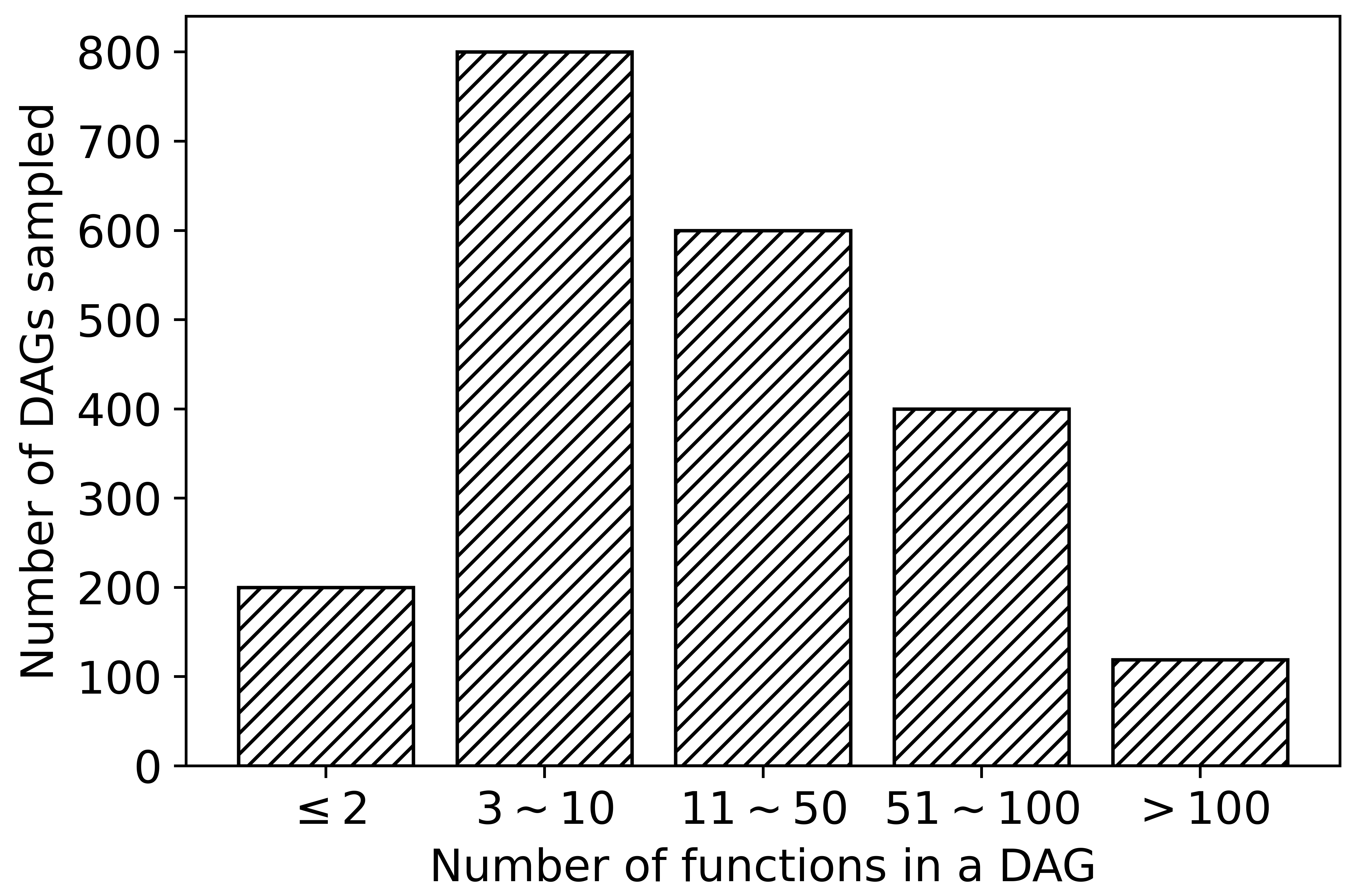
IoT stream processing workloads. The simulation is conducted based on Alibaba’s cluster trace of data analysis. This dataset contains more than 3 million jobs (called applications in this work), and 20365 jobs with unique DAG information. Considering that there are too many DAGs with only single-digit functions, we sampled 2119 DAGs with different size from the dataset. The distribution of the samples is visualized in Fig. 5. For each $f\in\mathcal{F}$ , the processing power required and output data size are extracted from the corresponding job in the dataset and scaled to $[1,10]$ giga flop and $[5,15]\times 10^{3}$ kbits, respectively.

Heterogenous edge servers. In our simulation, the number of edge servers is $10$ in default. Considering that the edge servers are required to formulate a connected graph, the impact of the sparsity of the graph is also studied. The processing power of edge servers and the maximum throughput of physical links are uniformly sampled from $[20,40]$ giga flop and $[30,80]\times 10^{3}$ kbit/s in default, respectively.

Algorithms compared. We compare DPE with the following algorithms.

•

FixDoc [1]: FixDoc is a function placement and DAG scheduling algorithm with fixed function configuration. FixDoc places each function onto homogeneous edge servers optimally to minimize the DAG completion time. Actually, [1] also proposes an improved version, GenDoc, with function configuration optimized, too. However, for IoT streaming processing scenario, on-demand function configuration is not applicative. Thus, we only compare DPE with FixDoc.
•

Heterogeneous Earliest-Finish-Time (HEFT) [8]: HEFT is a heuristic to schedule a set of dependent functions onto heterogenous workers with communication time taken into account. Starting with the highest priority, functions are assigned to different workers to heuristically minimize the overall completion time. HEFT is an algorithm that stands the test of time.

V-B Experiment Results

All the experiments are implemented in Python 3.7 on macOS Catalina equipped with 3.1 GHz Quad-Core Intel Core i7 and 16 GB RAM.

V-B1 Theoretical Performance Verification

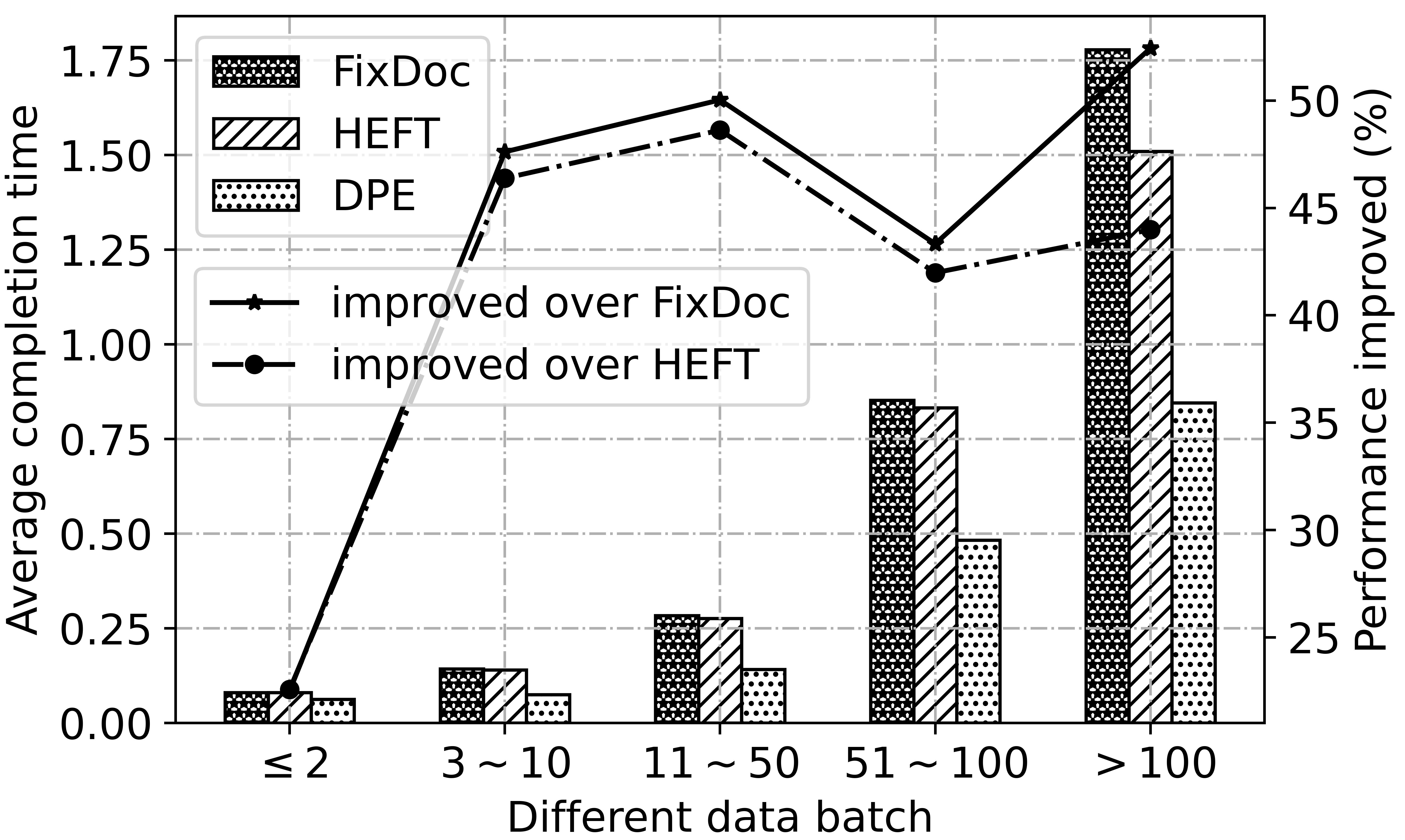
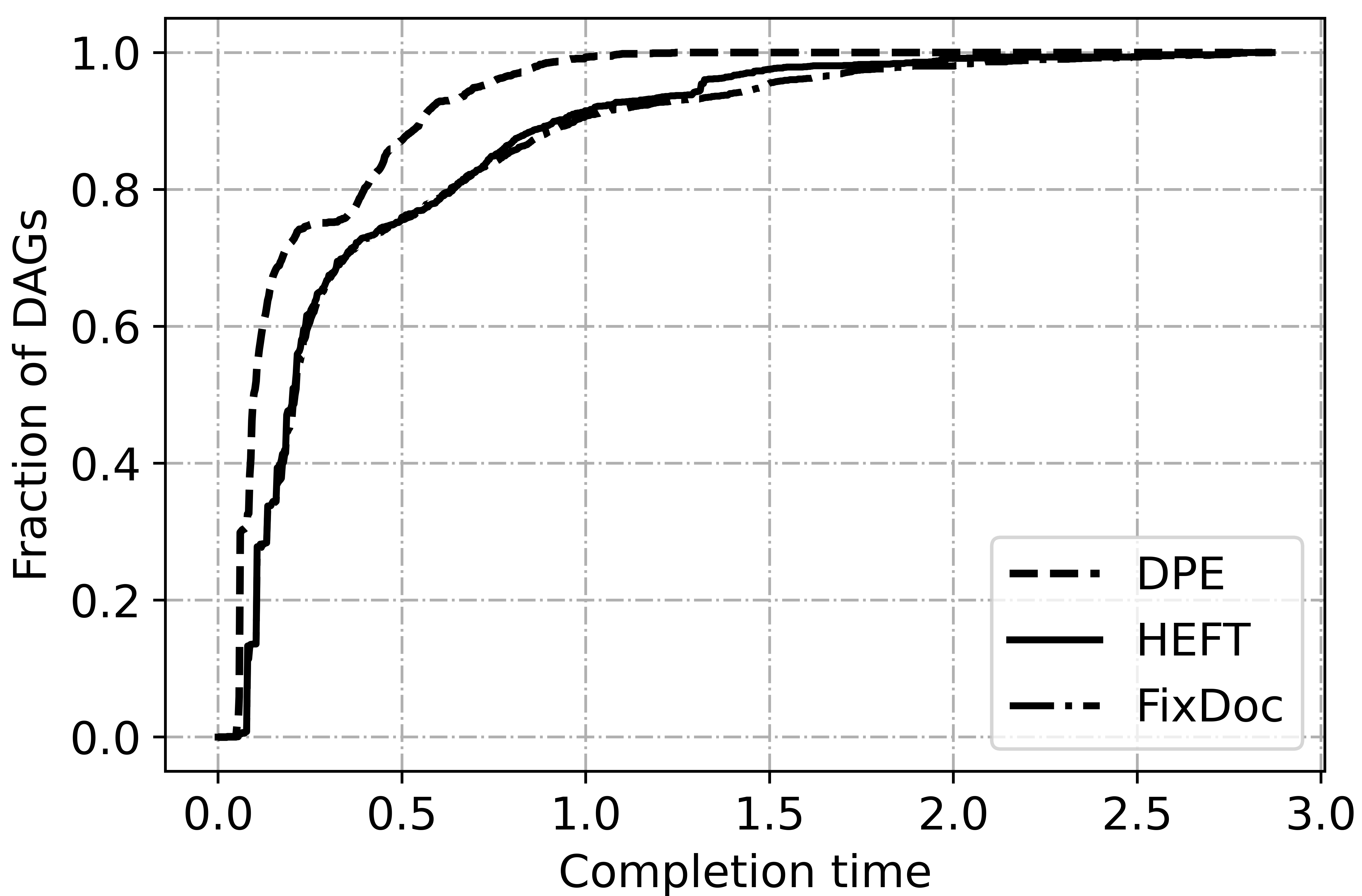
Fig. 6 illustrates the overall performance of the three algorithms. For different data batch, DPE can reduce $43.19\%$ and $40.71\%$ of the completion time on average over FixDoc and HEFT on 2119 DAGs. The advantage of DPE is more obvious when the scale of DAG is large because the parallelism is fully guaranteed. Fig. 7 shows the accumulative distribution of 2119 DAGs’ completion time. DPE is superior to HEFT and FixDoc on $100\%$ of the DAGs. Specifically, the maximum completion of DAG achieved by DPE is $1.24$ s. By contrast, only less $90\%$ of DAGs’ completion time achieved by HEFT and FixDoc can make it. The results verify the optimality of DPE.

Fig. 6 and Fig. 7 verify the superiority of proactive stream mapping and data splitting. By spreading data streams over multiple links, transmission time is greatly reduced. Besides, the optimal substructure makes sure DPE can find the optimal placement of each function simultaneously.

V-B2 Scalability Analysis

Fig. 8 and Fig. 9 shows the impact of the scale of the heterogenous edge $\mathcal{G}$ . In Fig. 8, we can find that the average completion time achieved by all algorithms decreases as the edge server increases. The result is obvious because more idle servers are avaliable, which ensures that more functions can be executed in parallel without waiting. For all data batches, DPE achieves the best result. It is interesting to find that the gap between other algorithms and DPE get widened when the scale of $\mathcal{G}$ increases. This is because the avaliable simple paths become more and the data transmission time is reduced even further. Fig. 8 also demonstrates the run time of different algorithms. The results show that DPE has the minimum time overhead.

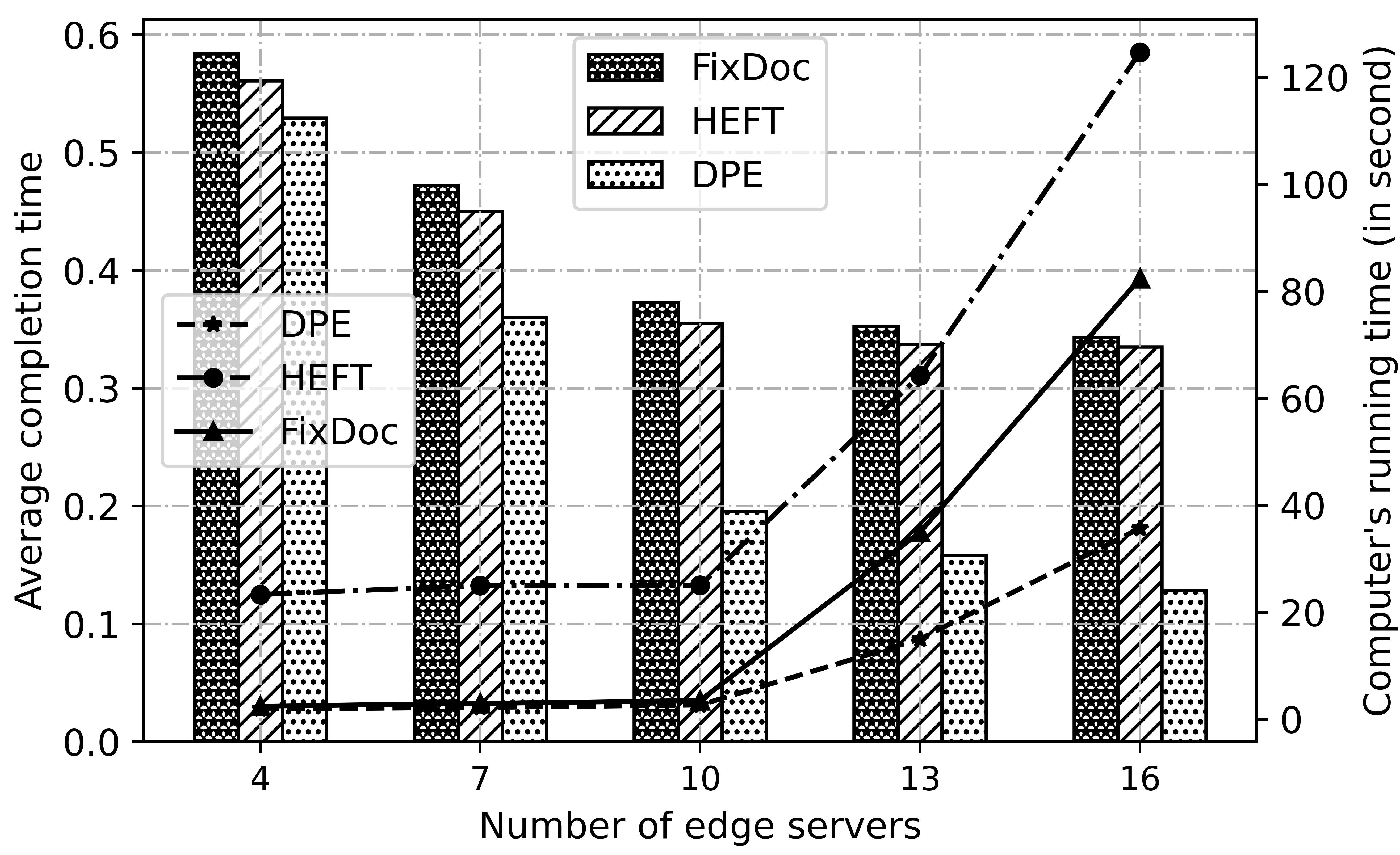
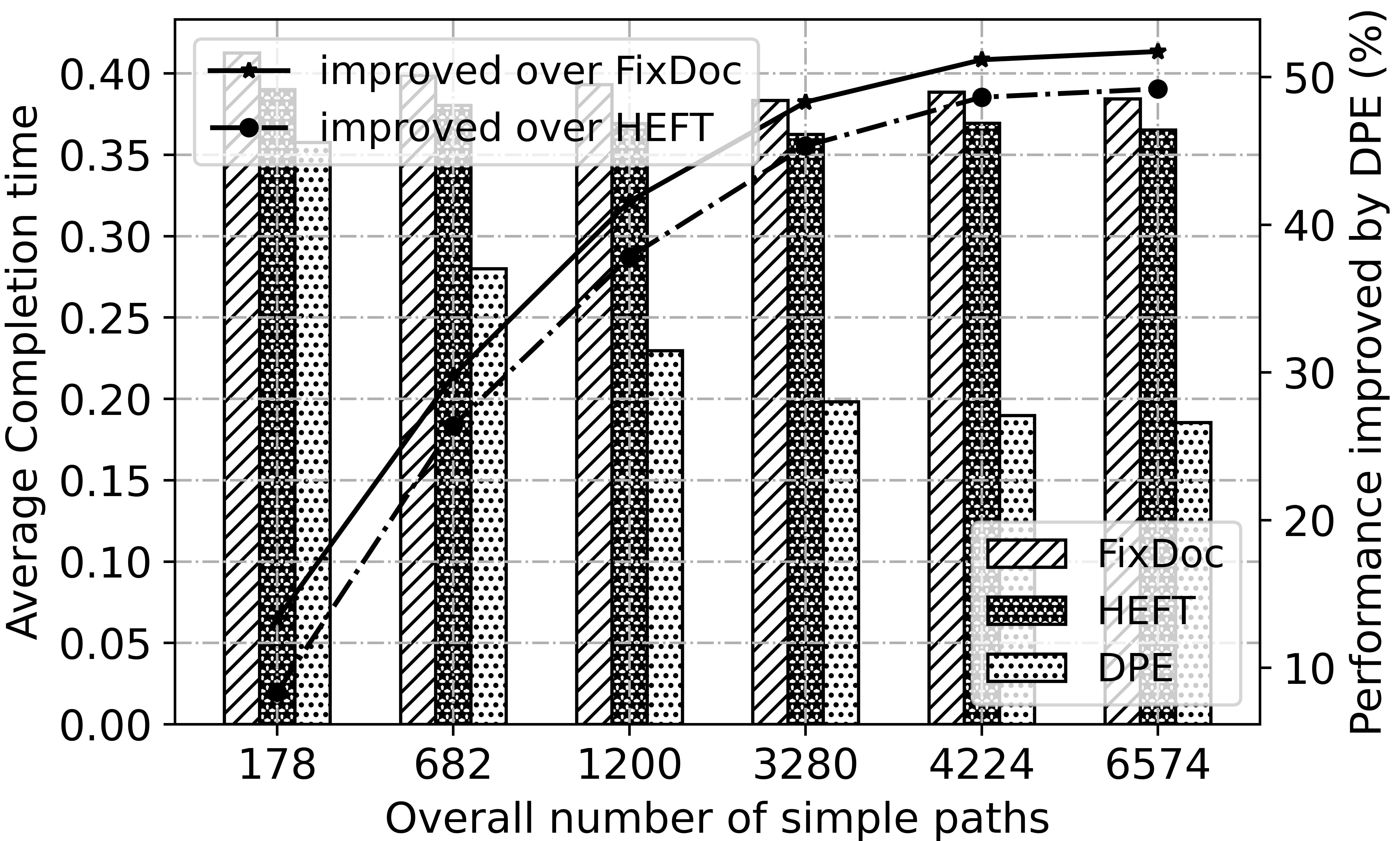
Fig. 9 show the impact of sparsity of $\mathcal{G}$ . The horizonal axis is the overall number of simple paths $\mathcal{G}$ . As it increases, $\mathcal{G}$ becomes more dense. because DPE can reduce transmission time with optimal data splitting and mapping, average completion time achieved by it decreases pretty evident. By contrast, FixDoc and HEFT have no obvious change.

V-B3 Sensitivity Analysis

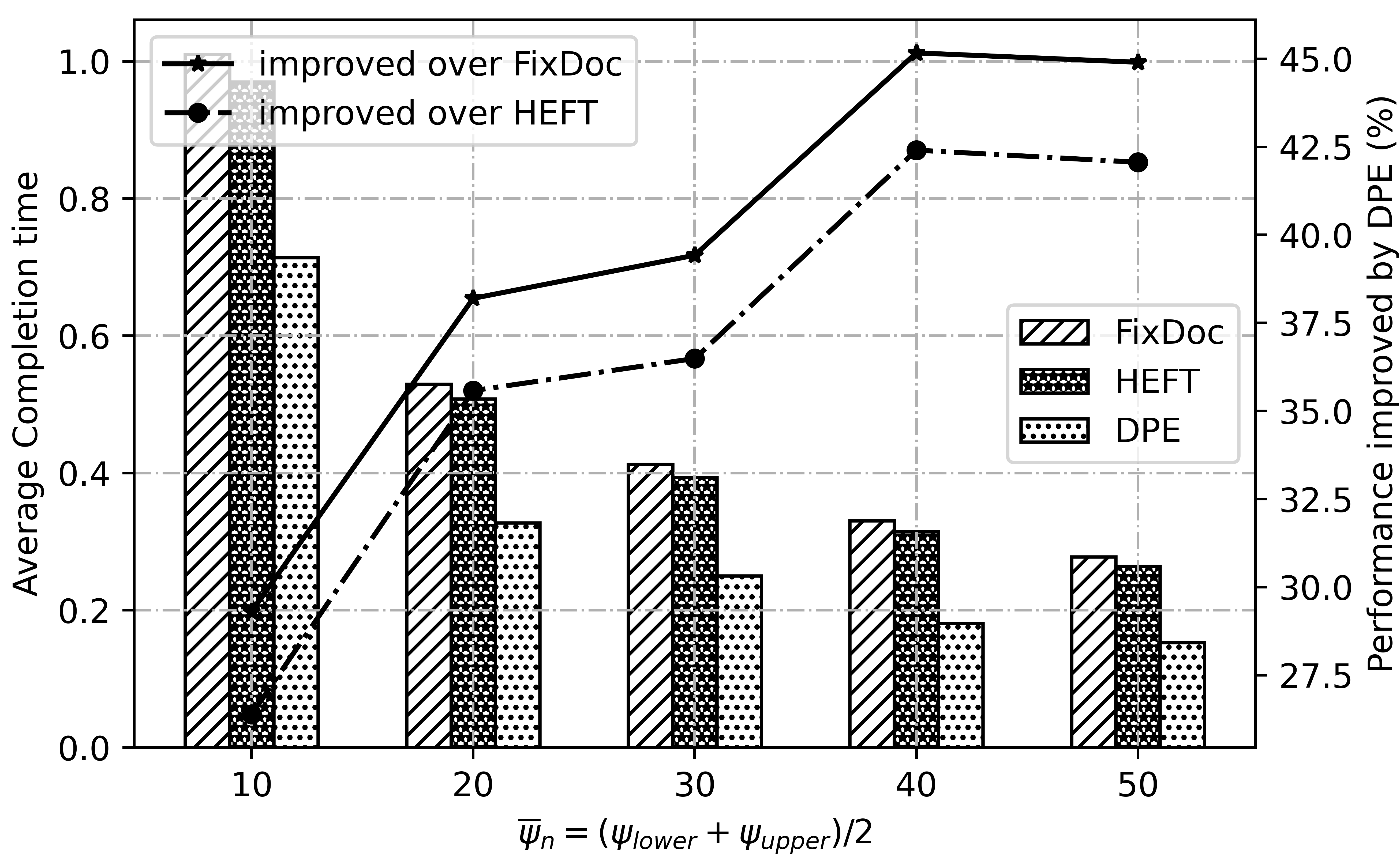
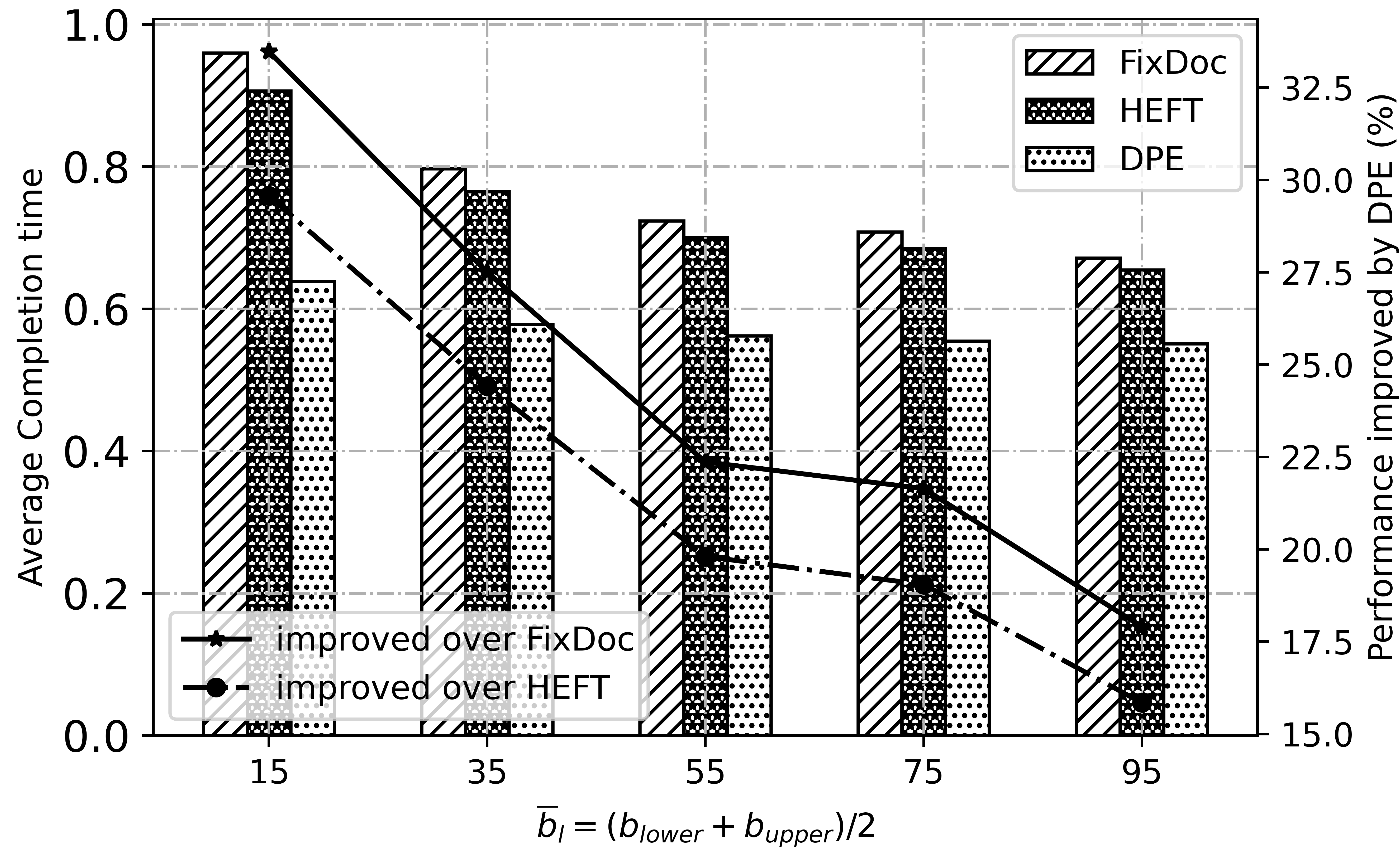
Fig. 10 and Fig. 11 demonstrate the impact of system parameters, $\psi_{n}$ and $b_{l}$ . Notice that $\forall n,l$ , $\psi_{n}$ and $b_{l}$ are sampled from the interval $[\psi_{lower},\psi_{upper}]$ and $[b_{lower},b_{upper}]$ uniformly, respectively. When the processing power and throughput increase, the computation and transmission time achieved by all algorithms are reduced. Even so, DPE outperforms all the other algorithms, which verifies the robustness of DPE adequately.

VI Related Works

In this section, we review related works on function placement and DAG scheduling at the network edge.

Studying the optimal function placement is not new. Since cloud computing paradigm became popular, it has been extensively studied in the literature [9][10]. When bringing function placement into the paradigm of edge computing, especially for the IoT stream processing, different constraints, such as the response time requirement of latency-critical applications, availability of function instances on the heterogenous edge servers, and the wireless and wired network throughput, etc., should be taken into consideration. In edge computing, the optimal function placement strategy can be used to maximize the network utility [11], minimize the inter-node traffic [12], minimize the makespan of the applications [1, 2, 3], or even minimize the budget of application service providers [13].

The application is either modeled as an individual blackbox or a DAG with complicated composite patterns. Considering that the IoT stream processing applications at the edge usually have interdependent correlations between the fore-and-aft functions, dependent function placement problem has a strong correlation with DAG dispatching and scheduling. Scheduling algorithms for edgy computation tasks have been extensively studied in recent years [8][14, 15, 16]. In edge computing, the joint optimization of DAG scheduling and function placement is usually NP-hard. As a result, many works can only achieve a near optimal solution based on heuristic or greedy policy. For example, Gedeon et al. proposed a heuristic-based solution for function placement across a three-tier edge-fog-cloud heterogenous infrastructure [17]. Cat et al. proposed a greedy algorithm for function placement by estimating the response time of paths in a DAG with queue theory [18]. Although FixDoc [1] can achieve the global optimal function placement, the completion time can be reduced further by optimizing the stream mapping.

VII Conclusion

This paper studies the optimal dependent function embedding problem. We first point out that proactive stream mapping and data splitting could have a strong impact on the makespan of DAGs with several use cases. Based on these observations, we design the DPE algorithm, which is theoretically verified to achieve the global optimality for an arbitrary DAG when the topological order of functions is given. DPE calls the RPF and the OSM algorithm to obtain the candidate paths and optimal stream mapping, respectively. Extensive simulations based on the Alibaba cluster trace dataset verify that our algorithms can reduce the makespan significantly compared with state-of-the-art function placement and scheduling methods, i.e., HEFT and FixDoc. The makespan can be further decreased by finding the optimal topological ordering and scheduling multiple DAGs simultaneously. We leave these extensions to our future work.

References

[1] L. Liu, H. Tan, S. H.-C. Jiang, Z. Han, X.-Y. Li, and H. Huang, “Dependent task placement and scheduling with function configuration in edge computing,” in Proceedings of the International Symposium on Quality of Service, ser. IWQoS ’19, New York, NY, USA, 2019.
[2] S. Khare, H. Sun, J. Gascon-Samson, K. Zhang, A. Gokhale, Y. Barve, A. Bhattacharjee, and X. Koutsoukos, “Linearize, predict and place: Minimizing the makespan for edge-based stream processing of directed acyclic graphs,” in Proceedings of the 4th ACM/IEEE Symposium on Edge Computing, ser. SEC ’19, New York, NY, USA, 2019, p. 1–14.
[3] Z. Zhou, Q. Wu, and X. Chen, “Online orchestration of cross-edge service function chaining for cost-efficient edge computing,” IEEE Journal on Selected Areas in Communications, vol. 37, no. 8, pp. 1866–1880, 2019.
[4] F. Duchene, D. Lebrun, and O. Bonaventure, “Srv6pipes: Enabling in-network bytestream functions,” Computer Communications, vol. 145, pp. 223 – 233, 2019.
[5] S. Vassilaras, L. Gkatzikis, N. Liakopoulos, I. N. Stiakogiannakis, M. Qi, L. Shi, L. Liu, M. Debbah, and G. S. Paschos, “The algorithmic aspects of network slicing,” IEEE Communications Magazine, vol. 55, no. 8, pp. 112–119, Aug 2017.
[6] I. Afolabi, T. Taleb, K. Samdanis, A. Ksentini, and H. Flinck, “Network slicing and softwarization: A survey on principles, enabling technologies, and solutions,” IEEE Communications Surveys Tutorials, vol. 20, no. 3, pp. 2429–2453, thirdquarter 2018.
[7] “Alibaba cluster trace program,” https://github.com/alibaba/clusterdata.
[8] H. Topcuoglu, S. Hariri, and Min-You Wu, “Performance-effective and low-complexity task scheduling for heterogeneous computing,” IEEE Transactions on Parallel and Distributed Systems, vol. 13, no. 3, pp. 260–274, 2002.
[9] G. T. Lakshmanan, Y. Li, and R. Strom, “Placement strategies for internet-scale data stream systems,” IEEE Internet Computing, vol. 12, no. 6, pp. 50–60, 2008.
[10] L. Tom and V. R. Bindu, “Task scheduling algorithms in cloud computing: A survey,” in Inventive Computation Technologies, S. Smys, R. Bestak, and Á. Rocha, Eds. Cham: Springer International Publishing, 2020, pp. 342–350.
[11] M. Leconte, G. S. Paschos, P. Mertikopoulos, and U. C. Kozat, “A resource allocation framework for network slicing,” in IEEE INFOCOM 2018 - IEEE Conference on Computer Communications, 2018, pp. 2177–2185.
[12] J. Xu, Z. Chen, J. Tang, and S. Su, “T-storm: Traffic-aware online scheduling in storm,” in 2014 IEEE 34th International Conference on Distributed Computing Systems, 2014, pp. 535–544.
[13] L. Chen, J. Xu, S. Ren, and P. Zhou, “Spatio–temporal edge service placement: A bandit learning approach,” IEEE Transactions on Wireless Communications, vol. 17, no. 12, pp. 8388–8401, 2018.
[14] Y. Kao, B. Krishnamachari, M. Ra, and F. Bai, “Hermes: Latency optimal task assignment for resource-constrained mobile computing,” IEEE Transactions on Mobile Computing, vol. 16, no. 11, pp. 3056–3069, 2017.
[15] S. Sundar and B. Liang, “Offloading dependent tasks with communication delay and deadline constraint,” in IEEE INFOCOM 2018 - IEEE Conference on Computer Communications, 2018, pp. 37–45.
[16] J. Meng, H. Tan, C. Xu, W. Cao, L. Liu, and B. Li, “Dedas: Online task dispatching and scheduling with bandwidth constraint in edge computing,” in IEEE INFOCOM 2019 - IEEE Conference on Computer Communications, 2019, pp. 2287–2295.
[17] J. Gedeon, M. Stein, L. Wang, and M. Muehlhaeuser, “On scalable in-network operator placement for edge computing,” in 2018 27th International Conference on Computer Communication and Networks (ICCCN), 2018, pp. 1–9.
[18] X. Cai, H. Kuang, H. Hu, W. Song, and J. Lü, “Response time aware operator placement for complex event processing in edge computing,” in Service-Oriented Computing, C. Pahl, M. Vukovic, J. Yin, and Q. Yu, Eds. Cham: Springer International Publishing, 2018, pp. 264–278.

$\displaystyle\min_{\mathbf{z}}\\|\mathbf{A}\mathbf{z}\\|_{\infty}$	$\displaystyle=$	$\displaystyle\lim_{x\to\infty}\sqrt[x]{\|\mathbf{\Omega}\|}\cdot\sqrt[\|\mathbf{\Omega}\|]{\prod_{k=1}^{\|\mathbf{\Omega}\|}A_{k,k}\mathbf{z}^{(k)}}$
	$\displaystyle=$	$\displaystyle\sqrt[\|\mathbf{\Omega}\|]{\prod_{k=1}^{\|\mathbf{\Omega}\|}A_{k,k}\mathbf{z}^{(k)}}\quad\rhd\textrm{with \eqref{P_map_cons}}$
	$\displaystyle=$	$\displaystyle\frac{s_{ij}}{\sum_{k=1}^{\|\mathbf{\Omega}\|}1/A_{k,k}}.$