Planar equilibrium measure problem
in the quadratic fields with a point charge

Sung-Soo Byun Center for Mathematical Challenges, Korea Institute for Advanced Study, 85 Hoegiro, Dongdaemun-gu, Seoul 02455, Republic of Korea sungsoobyun@kias.re.kr

(Date: March 15, 2025)

Abstract.

We consider a two-dimensional equilibrium measure problem under the presence of quadratic potentials with a point charge and derive the explicit shape of the associated droplets. This particularly shows that the topology of the droplets reveals a phase transition: (i) in the post-critical case, the droplets are doubly connected domain; (ii) in the critical case, they contain two merging type singular boundary points; (iii) in the pre-critical case, they consist of two disconnected components. From the random matrix theory point of view, our results provide the limiting spectral distribution of the complex and symplectic elliptic Ginibre ensembles conditioned to have zero eigenvalues, which can also be interpreted as a non-Hermitian extension of the Marchenko-Pastur law.

Key words and phrases:

Planar equilibrium measure problem, two-dimensional Coulomb gases, elliptic Ginibre ensemble, conditional point process, conformal mapping method, a non-Hermitian extension of the Marchenko-Pastur law

Sung-Soo Byun was partially supported by Samsung Science and Technology Foundation (SSTF-BA1401-51) and by the National Research Foundation of Korea (NRF-2019R1A5A1028324) and by a KIAS Individual Grant (SP083201) via the Center for Mathematical Challenges at Korea Institute for Advanced Study.

1. Introduction and Main results

In this paper, we study a planar equilibrium problem with logarithmic interaction under the influence of quadratic potentials with a point charge. This problem is purely deterministic, but its motivation comes from the random world, more precisely, from the random matrix theory or the theory of two-dimensional Coulomb gases in general. To be more concrete, for given points $\boldsymbol{\zeta}=(\zeta_{j})_{j=1}^{N}\in\mathbb{C}^{N}$ of configurations, we consider the Hamiltonians

(1.1)		$\displaystyle\mathbf{H}_{N}^{\mathbb{C}}(\boldsymbol{\zeta})$	$\displaystyle:=\sum_{1\leq j<k\leq N}\log\frac{1}{\|\zeta_{j}-\zeta_{k}\|^{2}}+N\sum_{j=1}^{N}W(\zeta_{j}),$
(1.2)		$\displaystyle\mathbf{H}_{N}^{\mathbb{H}}(\boldsymbol{\zeta})$	$\displaystyle:=\sum_{1\leq j<k\leq N}\log\frac{1}{\|\zeta_{j}-\zeta_{k}\|^{2}}+\sum_{1\leq j\leq k\leq N}\log\frac{1}{\|\zeta_{j}-\bar{\zeta}_{k}\|^{2}}+2N\sum_{j=1}^{N}W(\zeta_{j}).$

Here $W:\mathbb{C}\to{\mathbb{R}}$ is a suitable function called the external potential. These are building blocks to define joint probability distributions

(1.3)

d\mathbb{P}_{N,\beta}^{\mathbb{C}}(\boldsymbol{\zeta})\propto e^{-\frac{\beta}{2}\mathbf{H}_{N}^{\mathbb{C}}(\boldsymbol{\zeta})}\prod_{j=1}^{N}\,dA(\zeta_{j}),\qquad d\mathbb{P}_{N,\beta}^{\mathbb{H}}(\boldsymbol{\zeta})\propto e^{-\frac{\beta}{2}\mathbf{H}_{N}^{\mathbb{H}}(\boldsymbol{\zeta})}\prod_{j=1}^{N}\,dA(\zeta_{j}),

where $dA(\zeta)=d^{2}\zeta/\pi$ is the area measure and $\beta>0$ is the inverse temperature. Both point processes $\mathbb{P}_{N,\beta}^{\mathbb{C}}$ and $\mathbb{P}_{N,\beta}^{\mathbb{H}}$ represent two-dimensional Coulomb gas ensembles [38, 55, 62]. In particular, if $\beta=2$ , they are also called determinantal and Pfaffian Coulomb gases respectively due to their special integrable structures, see [26, 28] for recent reviews on this topic. Furthermore, they have an interpretation as eigenvalues of non-Hermitian random matrices with unitary and symplectic symmetry. For instance, if $W(\zeta)=|\zeta|^{2}$ , the ensembles (1.3) corresponds to the eigenvalues of complex and symplectic Ginibre matrices [40].

One of the fundamental questions regarding such point processes is their macroscopic/global behaviours as $N\to\infty.$ For the case $\beta=2$ , this can be regarded as a problem determining the limiting spectral distribution of given random matrices. The classical results in this direction include the circular law for the Ginibre ensembles. As expected from the structure of the Hamiltonians (1.1) and (1.2), the macroscopic behaviours of the system can be effectively described using the logarithmic potential theory [59].

For this purpose, let us briefly recap some basic notions in the logarithmic potential theory. Given a compactly supported probability measure $\mu$ on $\mathbb{C}$ , the weighted logarithmic energy $I_{W}[\mu]$ associated with the potential $W$ is given by

(1.4)

I_{W}[\mu]:=\int_{\mathbb{C}^{2}}\log\frac{1}{|z-w|}\,d\mu(z)\,d\mu(w)+\int_{\mathbb{C}}W\,d\mu.

For a general potential $W$ satisfying suitable conditions, there exists a unique probability measure $\mu_{W}$ which minimises $I_{W}[\mu]$ . Such a minimiser $\mu_{W}$ is called the equilibrium measure associated with $W$ and its support $S_{W}:=\operatorname{supp}(\mu_{W})$ is called the droplet. Furthermore, if $W$ is $C^{2}$ -smooth in a neighbourhood of $S_{W}$ , it follows from Frostman’s theorem that $\mu_{W}$ is absolutely continuous with respect to $dA$ and takes the form

(1.5)

d\mu_{W}(z)=\Delta W(z)\cdot\mathbbm{1}_{\{z\in S_{W}\}}\,dA(z),

where $\Delta:=\partial\bar{\partial}$ is the quarter of the usual Laplacian.

In relation with the point processes (1.3), it is well known [31, 15, 41] that

(1.6)

\mu_{N,W}:=\frac{1}{N}\sum_{j=1}^{N}\delta_{\zeta_{j}}\to\mu_{W}

in the weak star sense of measure. From the statistical physics viewpoint, this convergence is quite natural since the weighted energy $I_{W}$ in (1.4) corresponds to the continuum limit of the discrete Hamiltonians (1.1) and (1.2) after proper renormalisations. (In the case of (1.2), it is required to further assume that $W(\zeta)=W(\bar{\zeta})$ .)

Contrary to the density (1.5) of the measure $\mu_{W}$ , there is no general theory on the determination of its support $S_{W}$ . (See however [60] for a general theory on the regularity and [49] on the connectivity of the droplet associated with Hele-Shaw type potentials.) This leads to the following natural question.

For a given potential $W$ , what is the precise shape of the associated droplet?

In view of the energy functional (1.4), this is a typical form of an inverse problem in the potential theory and is called an equilibrium measure problem. Beyond the case when $W$ is radially symmetric (cf. [59, Section IV.6]), this problem is highly non-trivial even for some explicit potentials with a simple form, see [3, 12, 44, 14, 21, 35, 54, 36] for some recent works. Let us also stress that such a problem is important not only because it provides the intrinsic macroscopic behaviours of the point processes (1.3) but also because it plays the role of the first step to perform the Riemann-Hilbert analysis which gives rise to a more detailed statistical information ( $k$ -point functions) of the point processes, see [12, 13, 17, 18, 44, 45, 46, 47, 51, 53, 56] for extensive studies in this direction. In this work, we aim to contribute to the equilibrium problems associated with the potentials (1.7) and (1.14) below, which are of particular interest in the context of non-Hermitian random matrix theory.

1.1. Main results

For given parameters $\tau\in[0,1)$ and $c\geq 0$ , we consider the potential

(1.7)

Q(\zeta):=\frac{1}{1-\tau^{2}}\Big{(}|\zeta|^{2}-\tau\operatorname{Re}\zeta^{2}\Big{)}-2c\log|\zeta|.

When $\beta=2$ , the ensembles (1.3) associated with $Q$ correspond to the distribution of random eigenvalues of the elliptic Ginibre matrices of size $(c+1)N$ conditioned to have zero eigenvalues with multiplicity $cN$ . We mention that such a model with $c>0$ was also studied in the context of Quantum Chromodynamics [1].

In (1.7), the logarithmic term can be interpreted as an insertion of a point charge, see [4, 33, 23, 22, 27] for recent investigations of the models (1.3) in this situation. Such insertion of a point charge has also been studied in the theory of planar orthogonal polynomials [12, 13, 17, 51, 52, 53, 16]. On the other hand, the parameter $\tau\in[0,1)$ captures the non-Hermiticity of the model. To be more precise, the models (1.3) associated with $Q$ interpolate the complex/symplectic Ginibre ensembles ( $\tau=0$ ) with the Gaussian Unitary/Symplectic ensembles ( $\tau=1$ ) conditioned to have zero eigenvalues, see Remark 1.6 for further discussion in relation to our main results.

For the case $c=0$ , the terminology “elliptic” comes from the fact that the limiting spectrum $S_{\tau,0}$ is given by the ellipse

(1.8)

S_{\tau,0}:=\Big{\{}(x,y)\in{\mathbb{R}}^{2}:\Big{(}\frac{x}{1+\tau}\Big{)}^{2}+\Big{(}\frac{y}{1-\tau}\Big{)}^{2}\leq 1\Big{\}},

which is known as the elliptic law, see e.g. [34, 37]. We refer to [50, 5, 8, 57, 20, 19] and references therein for more about the recent progress on the complex elliptic Ginibre ensembles and [43, 6, 24, 25] for their symplectic counterparts. For the rotationally invariant case when $\tau=0,$ it is easy to show that the associated droplet $S_{0,c}$ is given by

(1.9)

S_{0,c}:=\Big{\{}(x,y)\in{\mathbb{R}}^{2}:c\leq x^{2}+y^{2}\leq 1+c\Big{\}},

see e.g. [59, Section IV.6] and [26, Section 5.2].

The primary goal of this work is to determine the precise shape of the droplet associated with the potential (1.7) for general $\tau\in[0,1)$ and $c\geq 0$ . For this, we set some notations. Let us write

(1.10)

\tau_{c}:=\frac{1}{1+2c}

for the critical non-Hermiticity parameter. For $\tau\in(\tau_{c},1)$ , we define

(1.11)

f(z)\equiv f_{\tau}(z):=\frac{(1+\tau)(1+2c)}{2}\frac{(1-az)(z-a\tau)^{2}}{z(z-a)},\qquad a=-\frac{1}{\sqrt{\tau(1+2c)}}.

We are now ready to present our main result.

Theorem 1.1.

Let $Q$ be given by (1.7). Then the droplet $S\equiv S_{\tau,c}=S_{Q}$ of the equilibrium measure

(1.12)

d\mu_{Q}(z)=\frac{1}{1-\tau^{2}}\mathbbm{1}_{S}(z)\,dA(z)

is given as follows.

•

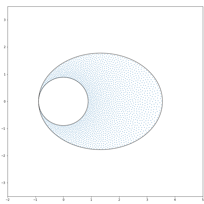
(Post-critical case) If $\tau\in(0,\tau_{c}]$ , we have

(1.13)

S_{\tau,c}=\Big{\{}(x,y)\in{\mathbb{R}}^{2}:\Big{(}\frac{x}{(1+\tau)\sqrt{1+c}}\Big{)}^{2}+\Big{(}\frac{y}{(1-\tau)\sqrt{1+c}}\Big{)}^{2}\leq 1\,,\,\frac{x^{2}+y^{2}}{(1-\tau^{2})c}\geq 1\Big{\}}.

•

(Pre-critical case) If $\tau\in[\tau_{c},1)$ , the droplet $S_{\tau,c}$ is the closure of the interior of the real analytic Jordan curves given by the image of the unit circle with respect to the map $z\mapsto\pm\sqrt{f(z)}$ , where $f$ is given by (1.11).

Refer to caption — (a) $\tau=1/6<\tau_{c}$

Note that if $c=0$ (resp., $\tau=0$ ), the droplet (1.13) corresponds to (1.8) (resp., (1.9)). We mention that the post-critical case of Theorem 1.1 is indeed shown in a more general setup, see (2.1) and Proposition 2.1 below.

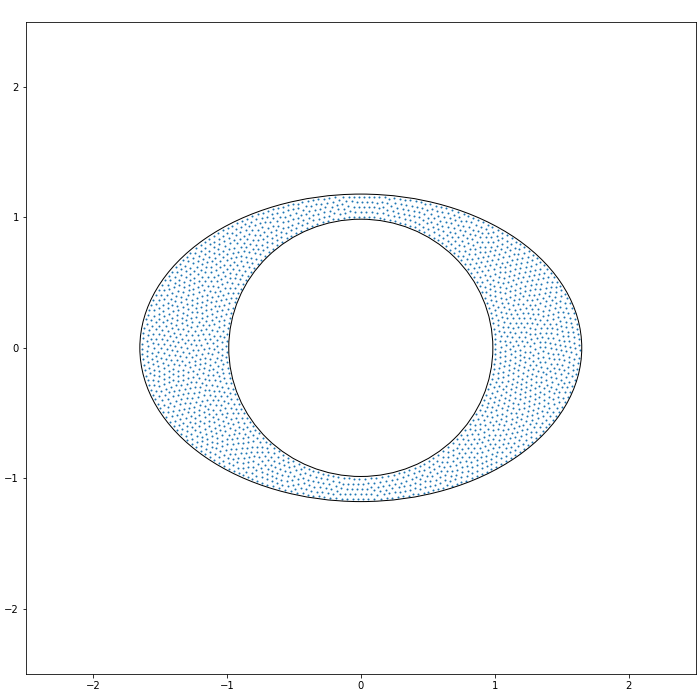
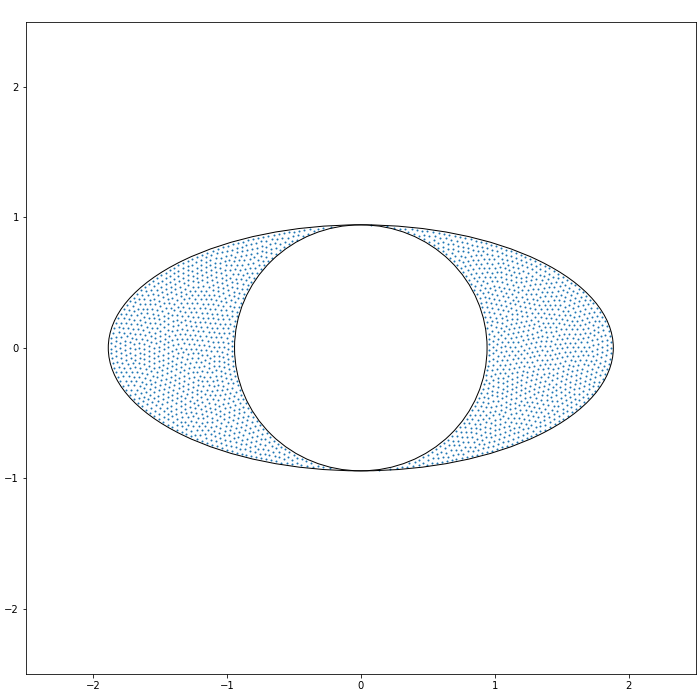
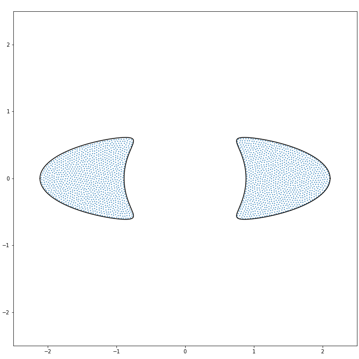
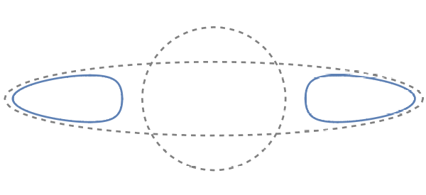
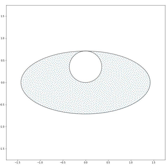
Remark 1.2 (Phase transition of the droplet).

In Theorem 1.1, we observe that if $c>0$ , the topology of the droplet reveals a phase transition. Namely, for the post-critical case when $\tau<\tau_{c}$ , the droplet is a doubly connected domain, whereas for the pre-critical case $\tau>\tau_{c}$ , it consists of two disconnected components. At criticality when $\tau=\tau_{c}$ , the droplet contains two symmetric double points. We refer to [12, 14, 3, 36] for further models whose droplets reveal various phase transitions. Let us also mention that recently, there have been several works on the models (1.3) with multi-component droplets, see e.g. [13, 30, 9, 10]. In this pre-critical regime, some theta-function oscillations are expected to appear for various kinds of statistics; cf. [32, 9]. The precise asymptotic behaviours of the partition function would also be interesting in connection with the conjecture that these depend on the Euler index of the droplets, see [42, 29] and [26, Sections 4.1 and 5.3] for further discussion.

Remark 1.3 (Fekete points and numerics).

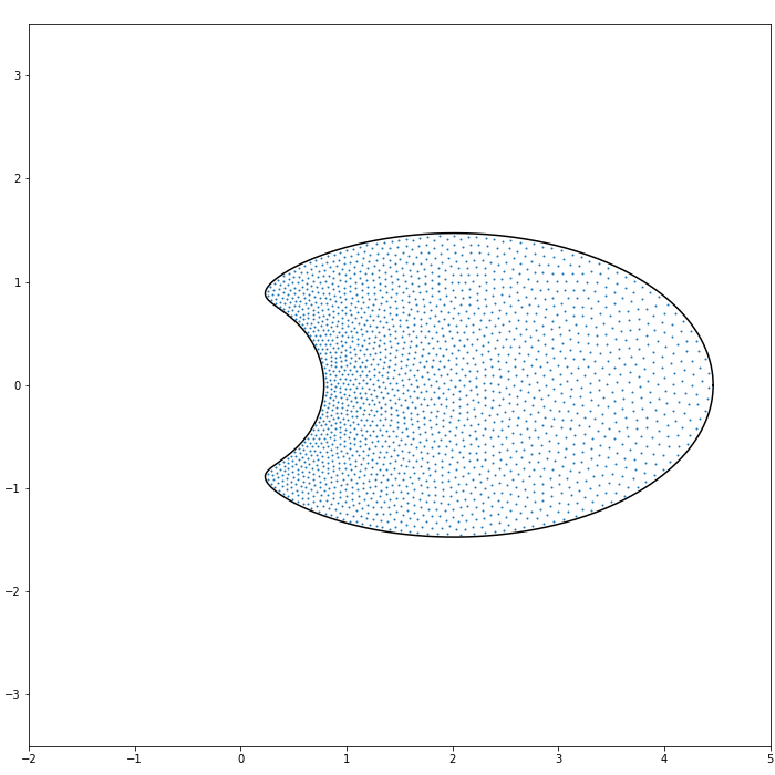
A configuration $\{\zeta_{j}\}_{j=1}^{N}$ which makes the Hamiltonians (1.1) or (1.2) minimal is known as a Fekete configuration. This can be interpreted as the ensembles (1.3) with low temperature limit $\beta=\infty$ , see e.g. [61, 58, 7, 11] and references therein. Since the droplet is independent of the inverse temperature $\beta>0$ (excluding the high-temperature regime [2] when $\beta=O(1/N)$ ), the Fekete points are useful to numerically observe the shape of the droplets. In Figures 1 and 2, Fekete configurations associated with the Hamiltonian (1.1) are also presented, which show good fits with Theorems 1.1 and 1.4.

Notice that the potential (1.7) and the droplet $S_{\tau,c}$ are invariant under the map $\zeta\mapsto-\zeta$ . We now discuss an equivalent formulation of Theorem 1.1 under the removal of such symmetry. (See [36, Section 1.3] for a similar discussion in a vector equilibrium problem on a sphere with point charges.) The motivation for this formulation will be clear in the next subsection.

For this purpose, we denote

(1.14)

\widehat{Q}(\zeta):=\frac{2}{1-\tau^{2}}\Big{(}|\zeta|-\tau\operatorname{Re}\zeta\Big{)}-2c\log|\zeta|.

By definition, the potentials $Q$ in (1.7) and $\widehat{Q}$ in (1.14) are related as

(1.15)

Q(\zeta)=\frac{1}{2}\widehat{Q}(\zeta^{2}).

Denoting by $\widehat{S}$ the droplet associated with $\widehat{Q}$ , it follows from [14, Lemma 1] that

(1.16)

S=\{\zeta\in\mathbb{C}:\zeta^{2}\in\widehat{S}\}.

Due to the relation (1.16) and

(1.17)

\Delta\widehat{Q}(\zeta)=\frac{1}{2(1-\tau^{2})}\frac{1}{|\zeta|},

we have the following equivalent formulation of Theorem 1.1.

Theorem 1.4.

Let $\widehat{Q}$ be given by (1.14). Then the droplet $\widehat{S}\equiv\widehat{S}_{\tau,c}=S_{\widehat{Q}}$ of the equilibrium measure

(1.18)

d\mu_{\widehat{Q}}(\zeta)=\frac{1}{2(1-\tau^{2})}\frac{1}{|\zeta|}\mathbbm{1}_{\widehat{S}}(\zeta)\,dA(\zeta)

is given as follows.

(i)

(Post-critical case) If $\tau\in(0,\tau_{c}]$ , we have

(1.19)

\widehat{S}_{\tau,c}=\Big{\{}(x,y)\in{\mathbb{R}}^{2}:\Big{(}\frac{x-2\tau(1+c)}{(1+\tau^{2})(1+c)}\Big{)}^{2}+\Big{(}\frac{y}{(1-\tau^{2})(1+c)}\Big{)}^{2}\leq 1\,,\,\frac{x^{2}+y^{2}}{(1-\tau^{2})^{2}c^{2}}\geq 1\Big{\}}.

(ii)

(Pre-critical case) If $\tau\in[\tau_{c},1)$ , the droplet $\widehat{S}_{\tau,c}$ is the closure of the interior of the real analytic Jordan curve given by the image of the unit circle with respect to the rational map $z\mapsto f(z)$ , where $f$ is given by (1.11).

Remark 1.5 (Joukowsky transform in the critical case).

If $\tau=\tau_{c}$ with (1.10), we have $a=1/a=-1$ . Thus in this critical case, the rational function $f_{\tau}$ in (1.11) is simplified as

(1.20)

f_{\tau_{c}}(z)=(1+c)\frac{(z+\tau)^{2}}{z}=(1+c)\Big{(}z+2\tau+\frac{\tau^{2}}{z}\Big{)}.

Note that compared to the general case (1.11), there is one less zero and one less pole in (1.20). Indeed, in the critical case, the rational map $f_{\tau_{c}}$ is a (shifted) Joukowsky transform

(1.21)

f_{\tau_{c}}:\mathbb{D}^{c}\to\Big{\{}(x,y)\in{\mathbb{R}}^{2}:\Big{(}\frac{x-2\tau(1+c)}{(1+\tau^{2})(1+c)}\Big{)}^{2}+\Big{(}\frac{y}{(1-\tau^{2})(1+c)}\Big{)}^{2}\geq 1\Big{\}}.

In [3], a similar type of Joukowsky transform was used to solve an equilibrium measure problem. For the models under consideration in the present work, due to a more complicated form of the rational function (1.11), the required analysis for the associated equilibrium problem turns out to be more involved.

Remark 1.6 (A non-Hermitian extension of the Marchenko-Pastur distribution).

In the Hermitian limit $\tau\uparrow 1,$ by (1.7) and (1.14), we have

(1.22)		$\displaystyle\lim_{\tau\uparrow 1}Q(x+iy)=V(x):=\begin{cases}\displaystyle\frac{x^{2}}{2}-2c\log\|x\|,&\text{if }y=0,\vskip 3.0pt plus 1.0pt minus 1.0pt\\ +\infty&\text{otherwise},\end{cases}$
(1.23)		$\displaystyle\lim_{\tau\uparrow 1}\widehat{Q}(x+iy)=\widehat{V}(x):=\begin{cases}\displaystyle x-2c\log\|x\|,&\text{if }y=0,\,x>0,\vskip 3.0pt plus 1.0pt minus 1.0pt\\ +\infty&\text{otherwise}.\end{cases}$

Then the associated equilibrium measures are given by the well-known Marchenko-Pastur law (with squared variables) [38, Proposition 3.4.1], i.e.

(1.24)		$\displaystyle d\mu_{V}(x)$	$\displaystyle=\frac{1}{2\pi\|x\|}\,\sqrt{(\lambda_{+}^{2}-x^{2})(x^{2}-\lambda_{-}^{2})}\cdot\mathbbm{1}_{[-\lambda_{+},-\lambda_{-}]\cup[\lambda_{-},\lambda_{+}]}\,dx,$
(1.25)		$\displaystyle d\mu_{\widehat{V}}(x)$	$\displaystyle=\frac{1}{2\pi x}\,\sqrt{(\lambda_{+}^{2}-x)(x-\lambda_{-}^{2})}\cdot\mathbbm{1}_{[\lambda_{-}^{2},\lambda_{+}^{2}]}\,dx,$

where $\lambda_{\pm}:=\sqrt{2c+1}\pm 1$ , cf. Remark 2.3. Therefore one can interpret Theorem 1.1 (resp., Theorem 1.4) as a non-Hermitian generalisation of the Marchenko-Pastur distribution (1.24) (resp., (1.25)), see [8, Section 2] for more about the geometric meaning with the notion of the statistical cross-section. We also refer to [3] for another non-Hermitian extension of (1.24) and (1.25) in the context of the chiral Ginibre ensembles.

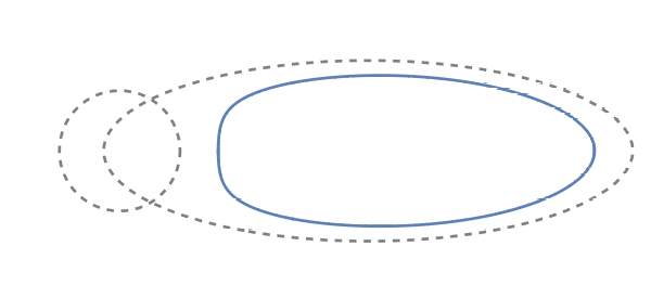
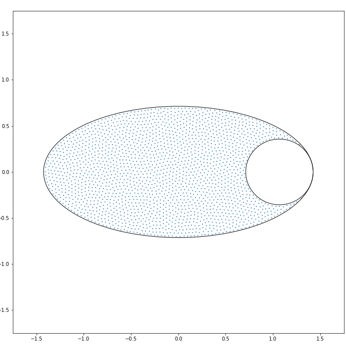
Remark 1.7 (Inclusion relations of the droplets).

Let us write

(1.26)

\displaystyle S_{1}=\Big{\{}(x,y)\in{\mathbb{R}}^{2}:\Big{(}\frac{x}{1+\tau}\Big{)}^{2}+\Big{(}\frac{y}{1-\tau}\Big{)}^{2}\leq 1+c\Big{\}},\qquad S_{2}:=\Big{\{}(x,y)\in{\mathbb{R}}^{2}:x^{2}+y^{2}\leq(1-\tau^{2})c\Big{\}}

and denote by $\widehat{S}_{j}$ $(j=1,2)$ the image of $S_{j}$ under the map $z\mapsto z^{2}$ . Then it follows from the definition (1.10) that

(1.27)

\tau\in(0,\tau_{c})\qquad\textup{if and only if}\qquad S_{1}^{c}\cap S_{2}=\emptyset.

By Theorems 1.1 and 1.4, for general $\tau\in[0,1)$ and $c\geq 0$ , one can observe that

(1.28)

S_{\tau,c}\subseteq S_{1}\cap(\textup{Int}\,S_{2})^{c},\qquad\widehat{S}_{\tau,c}\subseteq\widehat{S}_{1}\cap(\textup{Int}\,\widehat{S}_{2})^{c}.

Here, equality in (1.28) holds if and only if in the post-critical case. (This property holds in a more general setup, see Proposition 2.1.) On the other hand, in the pre-critical case one can interpret that the particles in $S_{1}^{c}\cap S_{2}$ are smeared out to $S_{1}\cap S_{2}^{c}$ which makes the inclusion relations (1.28) strictly hold, see Figure 3.

1.2. Outline of the proof

Recall that $\mu_{W}$ is a unique minimiser of the energy (1.4). It is well known that the equilibrium measure $\mu_{W}$ is characterised by the variational conditions (see [59, p.27])

(1.29)		$\displaystyle\int\log\frac{1}{\|\zeta-z\|^{2}}\,d\mu_{W}(z)+W(\zeta)=C,\quad\text{q.e.}\quad\text{if }\zeta\in S_{W};\vskip 3.0pt plus 1.0pt minus 1.0pt$
(1.30)		$\displaystyle\int\log\frac{1}{\|\zeta-z\|^{2}}\,d\mu_{W}(z)+W(\zeta)\geq C,\quad\text{q.e.}\quad\text{if }\zeta\notin S_{W}.$

Here, q.e. stands for quasi-everywhere. (Nevertheless, this notion is not important in the sequel as we will show that for the models we consider the conditions (1.29) and (1.30) indeed hold everywhere.)

Due to the uniqueness of the equilibrium measure, all we need to show is that if $W=Q$ , then $\mu_{Q}$ in (1.12) satisfies the variational principles (1.29) and (1.30). Equivalently, by (1.16), it also suffices to show the variational principles for the equilibrium measure $\mu_{\widehat{Q}}$ in (1.18).

However, it is far from being obvious to obtain the “correct candidate” of the droplets. Perhaps one may think that at least for the post-critical case, the shape of the droplet (1.13) is quite natural given the well-known cases (1.8) and (1.9) as well as the fact that the area of $S_{\tau,c}$ should be $(1-\tau^{2})\pi$ . On the other hand, for the pre-critical case, one can easily notice that there is some secret behind deriving the explicit formula of the rational function (1.11). To derive the correct candidate, we use the conformal mapping method with the help of the Schwarz function, see Appendix A.

Remark 1.8 (Removal of symmetry).

We emphasise that the conformal mapping method does not work for the multi-component droplet, i.e. the pre-critical case of Theorem 1.1. This is essentially due to the lack of the Riemann mapping theorem. Nevertheless, one can observe that once we remove the symmetry $\zeta\mapsto-\zeta$ , the droplet in the pre-critical case of Theorem 1.4 is simply connected. This explains the reason why we need the idea of removing symmetry.

The rest of this paper is organised as follows.

•

In Section 2, we prove Theorems 1.1 and 1.4. In Subsection 2.1, we show the post-critical case of Theorem 1.1 in a more general setup, see Proposition 2.1. On the other hand, in Subsection 2.2, we show the pre-critical case of Theorem 1.4. Then by the relation (1.16), these complete the proof of our main results.
•

This article contains two appendices. In Appendix A, we explain the conformal mapping method to derive the “correct candidate” of the droplets. In Appendix B, we present a way to solve a one-dimensional equilibrium problem in Remark 2.3, which shares a common feature with the conformal mapping method. These appendices are made only for instructive purposes and the readers who only want the proof of the main theorems may stop at the end of Section 2.

2. Proof of main theorem

In this section, we show Theorems 1.1 and 1.4.

2.1. Post critical cases

Extending (1.7), we consider the potential

(2.1)

Q_{p}(\zeta):=\frac{1}{1-\tau^{2}}\Big{(}|\zeta|^{2}-\tau\operatorname{Re}\zeta^{2}\Big{)}-2c\log|\zeta-p|,\qquad p\in\mathbb{C}.

For the case $\tau=0$ , the shape of the droplet associated with the potential (2.1) was fully characterised in [12]. (In this case, it suffices to consider the case $p\geq 0$ due to the rotational invariance.) In particular, it was shown that if

(2.2)

c<\frac{(1-p^{2})^{2}}{4p^{2}},\qquad\tau=0,\qquad p\geq 0,

the droplet is given by $S=\overline{\mathbb{D}(0,\sqrt{1+c})}\setminus\mathbb{D}(p,\sqrt{c}),$ where $\mathbb{D}(p,R)$ is the disc with centre $p$ and radius $R$ , cf. see Remark A.5 for the other case $c>(1-p^{2})^{2}/(4p^{2})$ .

To describe the droplets associated with $Q_{p}$ , we denote

(2.3)

S_{1}:=\Big{\{}(x,y)\in{\mathbb{R}}^{2}:\Big{(}\frac{x}{1+\tau}\Big{)}^{2}+\Big{(}\frac{y}{1-\tau}\Big{)}^{2}\leq 1+c\Big{\}}

and

(2.4)

S_{2}:=\Big{\{}(x,y)\in{\mathbb{R}}^{2}:(x-\operatorname{Re}p)^{2}+(y-\operatorname{Im}p)^{2}\leq(1-\tau^{2})c\Big{\}}.

Then we obtain the following.

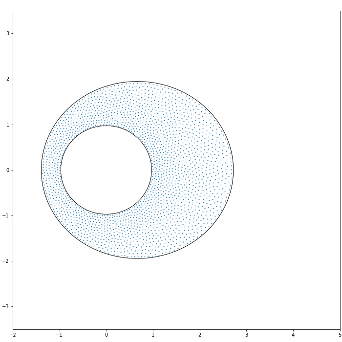
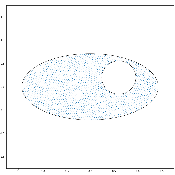
Proposition 2.1.

Suppose that the parameters $\tau,c\in{\mathbb{R}}$ and $p\in\mathbb{C}$ are given to satisfy

(2.5)

S_{2}\subset S_{1},

where $S_{1}$ and $S_{2}$ are given by (2.3) and (2.4). Then the droplet $S\equiv S_{Q_{p}}$ associated with (2.1) is given by

(2.6)

S=S_{1}\cap(\textup{Int}\,S_{2})^{c}.

See Figure 4 for the shape of the droplets and numerical simulations of Fekete point configurations. We remark that with slight modifications, Proposition 2.1 can be further extended to the case with multiple point charges, i.e. the potential of the form

(2.7)

\frac{1}{1-\tau^{2}}\Big{(}|\zeta|^{2}-\tau\operatorname{Re}\zeta^{2}\Big{)}-2\sum c_{j}\log|\zeta-p_{j}|,\qquad p_{j}\in\mathbb{C},\quad c_{j}\geq 0.

(See Remark A.4 for a related discussion.) Let us also mention that a similar statement for an equilibrium problem on the sphere was shown in [21]. For a treatment of a more general case, we refer the reader to [35, 54, 36].

Remark 2.2.

If $p=0$ , the condition (2.5) corresponds to

(2.8)

\tau<\frac{1}{1+2c}=\tau_{c}.

Therefore Proposition 2.1 for the special value $p=0$ gives Theorem 1.1 (i). As a consequence, by (1.16), Theorem 1.4 (i) also follows. We also mention that if $\tau=0$ and $p>0$ , the condition (2.5) coincides with (2.2).

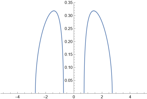
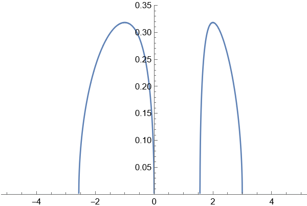
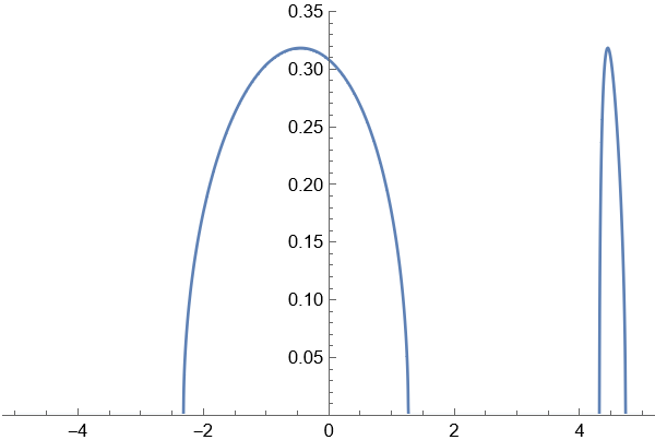
Remark 2.3 (Equilibrium measure in the Hermitian limit).

Before moving on to the planar equilibrium problem for (2.1), we first discuss the one-dimensional problem arising in the Hermitian limit. For $p\in{\mathbb{R}}$ , the Hermitian limit $\tau\uparrow 1$ of the potential $Q_{p}$ is given by

(2.9)

\lim_{\tau\uparrow 1}Q_{p}(x+iy)=V_{p}(x):=\begin{cases}\displaystyle\frac{x^{2}}{2}-2c\log|x-p|,&\text{if }y=0,\vskip 3.0pt plus 1.0pt minus 1.0pt\\ +\infty&\text{otherwise}.\end{cases}

Then one can show that the associated equilibrium measure $\mu_{V}\equiv\mu_{V_{p}}$ is given by

(2.10)

\frac{d\mu_{V}(x)}{dx}=\frac{\sqrt{-\prod_{j=1}^{4}(x-\lambda_{j})}}{2\pi|x-p|}\cdot\mathbbm{1}_{[\lambda_{1},\lambda_{2}]\cup[\lambda_{3},\lambda_{4}]}(x),

where

(2.11)		$\displaystyle\lambda_{1}=\frac{p-2-\sqrt{(p+2)^{2}+8c}}{2},\qquad\lambda_{2}=\frac{p+2-\sqrt{(p-2)^{2}+8c}}{2},$
(2.12)		$\displaystyle\lambda_{3}=\frac{p-2+\sqrt{(p+2)^{2}+8c}}{2},\qquad\lambda_{4}=\frac{p+2+\sqrt{(p-2)^{2}+8c}}{2}.$

We remark that when $p=0$ , it recovers (1.24). See Figure 5 for the graphs of the equilibrium measure $\mu_{V_{p}}$ . The equilibrium measure (2.10) follows from the standard method using the Stieltjes transform and the Sokhotski-Plemelj inversion formula. For reader’s convenience, we provide a proof of (2.10) in Appendix B.

In the rest of this subsection, we prove Proposition 2.1. First, let us show the following elementary lemmas.

Lemma 2.4.

For $a,b>0$ , let

K:=\Big{\{}(x,y)\in{\mathbb{R}}^{2}:\Big{(}\frac{x}{a}\Big{)}^{2}+\Big{(}\frac{y}{b}\Big{)}^{2}\leq 1\Big{\}}.

Then we have

(2.13)

\int_{K}\frac{1}{\zeta-z}\,dA(z)=\begin{cases}\displaystyle\bar{\zeta}-\frac{a-b}{a+b}\,\zeta&\text{if }\zeta\in K,\vskip 3.0pt plus 1.0pt minus 1.0pt\\ \displaystyle\frac{2ab}{a^{2}-b^{2}}\Big{(}\zeta-\sqrt{\zeta^{2}-a^{2}+b^{2}}\Big{)}&\text{otherwise.}\end{cases}

In particular, for $\zeta\in K$ , there exists a constant $c_{0}\in{\mathbb{R}}$ such that

(2.14)

\int_{K}\log|\zeta-z|^{2}\,dA(z)=|\zeta|^{2}-\frac{a-b}{a+b}\operatorname{Re}\zeta^{2}+c_{0}.

Remark 2.5.

The Cauchy transform in (2.13) is useful to explicitly compute the moments of the equilibrium measure. Namely, by definition, we have

\int_{K}\frac{1}{\zeta-z}\,dA(z)=\frac{1}{\zeta}\sum_{k=0}^{\infty}\frac{1}{\zeta^{k}}\int_{K}z^{k}\,dA(z),\qquad\zeta\to\infty.

On the other hand, we have

\displaystyle\zeta-\sqrt{\zeta^{2}-a^{2}+b^{2}}=\frac{a^{2}-b^{2}}{\zeta}\sum_{k=0}^{\infty}\binom{1/2}{k+1}\frac{(b^{2}-a^{2})^{k}}{\zeta^{2k}},\qquad\zeta\to\infty.

Combining the above equations with (2.13), we obtain that for any non-negative integer $k,$

(2.15)

\frac{1}{ab}\int_{K}z^{2k}\,dA(z)=2\binom{1/2}{k+1}(b^{2}-a^{2})^{k}.

Proof of Lemma 2.4.

Recall that $\mathbb{D}$ is the unit disc with centre the origin. Then the Joukowsky transform $f:\bar{\mathbb{D}}^{c}\to K^{c}$ is given by

(2.16)

f(z)=\frac{a+b}{2}\,z+\frac{a-b}{2}\,\frac{1}{z}.

By applying Green’s formula, we have

(2.17)

\int_{K}\frac{1}{\zeta-z}\,dA(z)=\frac{1}{2\pi i}\int_{\partial K}\frac{\bar{z}}{\zeta-z}\,dz+\bar{\zeta}\cdot\mathbbm{1}_{\{\zeta\in K\}}.

Furthermore, by the change of variable $z=f(w)$ , it follows that

(2.18)

\displaystyle\int_{\partial K}\frac{\bar{z}}{\zeta-z}\,dz

\displaystyle=\int_{\partial\mathbb{D}}\frac{\overline{f(1/\bar{w})}}{\zeta-f(w)}f^{\prime}(w)\,dw=\int_{\partial\mathbb{D}}g_{\zeta}(w)\,dw,

where $g_{\zeta}$ is the rational function given by

(2.19)

g_{\zeta}(w):=\frac{1}{\zeta-f(w)}\Big{(}\frac{a+b}{2}\frac{1}{w}+\frac{a-b}{2}w\Big{)}\Big{(}\frac{a+b}{2}-\frac{a-b}{2}\frac{1}{w^{2}}\Big{)}.

Observe that

\zeta=f(w)\qquad\textrm{if and only if}\qquad w=w_{\zeta}^{\pm}:=\frac{\zeta\pm\sqrt{\zeta^{2}-a^{2}+b^{2}}}{a+b},

i.e. the points $w_{\zeta}^{\pm}$ are solutions to the quadratic equation

(a+b)w^{2}-2\zeta\,w+(a-b)=0.

Here, the branch of the square root is chosen such that

w_{\zeta}^{-}\to 0\qquad\zeta\to\infty.

By above observation, the function $g_{\zeta}$ has poles only at

0,\qquad w_{\zeta}^{+},\qquad w_{\zeta}^{-}.

Moreover note that

\zeta\in K\qquad\textrm{if and only if}\qquad w_{\zeta}^{\pm}\in\mathbb{D}.

Notice that if $\zeta\in K^{c}$ , then $w_{\zeta}^{-}\in\mathbb{D}$ and $w_{\zeta}^{+}\in\mathbb{D}^{c}$ .

Using the residue calculus, we have

(2.20)

\underset{w=0}{\textrm{Res}}\,\Big{[}g_{\zeta}(w)\Big{]}=\frac{a+b}{a-b}\,\zeta.

On the other hand, we have

(2.21)

\underset{w=w_{\zeta}^{\pm}}{\textrm{Res}}\,\Big{[}g_{\zeta}(w)\Big{]}=-\overline{f(1/\bar{w}_{\zeta}^{\pm})}=-\frac{a+b}{2}\frac{1}{w_{\zeta}^{\pm}}-\frac{a-b}{2}w_{\zeta}^{\pm}.

In particular,

(2.22)

\underset{w=w_{\zeta}^{+}}{\textrm{Res}}\,\Big{[}g_{\zeta}(w)\Big{]}+\underset{w=w_{\zeta}^{-}}{\textrm{Res}}\,\Big{[}g_{\zeta}(w)\Big{]}=-2\frac{a^{2}+b^{2}}{a^{2}-b^{2}}\,\zeta.

Combining all of the above, we obtain the desired identity (2.13). The second assertion immediately follows from (2.13) and the real-valuedness of $\zeta\mapsto\int_{K}\log|\zeta-z|^{2}\,dA(z)$ . ∎

Lemma 2.6.

For $R>0$ and $p\in\mathbb{C}$ we have

(2.23)

\int_{\mathbb{D}(p,R)}\log|\zeta-z|\,dA(z)=\begin{cases}\displaystyle R^{2}\log|\zeta-p|&\text{if }\zeta\notin\mathbb{D}(p,R),\vskip 3.0pt plus 1.0pt minus 1.0pt\\ \displaystyle R^{2}\log R-\frac{R^{2}}{2}+\frac{|\zeta-p|^{2}}{2}&\text{otherwise}.\end{cases}

Proof.

First, recall the well-known Jensen’s formula: for $r>0$ ,

(2.24)

\frac{1}{2\pi}\int_{0}^{2\pi}\log|\zeta-re^{i\theta}|\,d\theta=\begin{cases}\log r&\text{if }r>|\zeta|,\vskip 3.0pt plus 1.0pt minus 1.0pt\\ \log|\zeta|&\text{otherwise}.\end{cases}

By the change of variables, we have

\displaystyle\int_{\mathbb{D}(p,R)}\log|\zeta-z|\,dA(z)

\displaystyle=\int_{\mathbb{D}(0,R)}\log|\zeta-p-z|\,dA(z)=\frac{1}{\pi}\int_{0}^{R}r\int_{0}^{2\pi}\log|\zeta-p-re^{i\theta}|\,d\theta\,dr.

Suppose that $\zeta\notin\mathbb{D}(p,R)$ . Then by applying (2.24), we have

\displaystyle\frac{1}{\pi}\int_{0}^{R}r\int_{0}^{2\pi}\log|\zeta-p-re^{i\theta}|\,d\theta\,dr

\displaystyle=2\int_{0}^{R}r\,\log|\zeta-p|\,dr=R^{2}\log|\zeta-p|.

On the other hand if $\zeta\in\mathbb{D}(p,R)$ , we have

	$\displaystyle\frac{1}{\pi}\int_{0}^{R}r\int_{0}^{2\pi}\log\|\zeta-p-re^{i\theta}\|\,d\theta\,dr$	$\displaystyle=2\int_{0}^{\|\zeta-p\|}r\,\log\|\zeta-p\|\,dr+2\int_{\|\zeta-p\|}^{R}r\,\log r\,dr$
		$\displaystyle=R^{2}\log R-\frac{R^{2}}{2}+\frac{\|\zeta-p\|^{2}}{2},$

which completes the proof. ∎

We are now ready to complete the proof of Proposition 2.1.

Proof of Proposition 2.1.

Note that by (1.5), the equilibrium measure $\mu$ associated with $Q_{p}$ is of the form

(2.25)

d\mu(z):=\Delta Q_{p}(z)\cdot\mathbbm{1}_{S}(z)\,dA(z)=\frac{1}{1-\tau^{2}}\cdot\mathbbm{1}_{S}(z)\,dA(z).

Due to the assumption (2.5), we have

\displaystyle\int\log\frac{1}{|\zeta-z|^{2}}\,d\mu(z)=\frac{1}{1-\tau^{2}}\Big{(}\int_{S_{1}}\log\frac{1}{|\zeta-z|^{2}}\,dA(z)-\int_{S_{2}}\log\frac{1}{|\zeta-z|^{2}}\,dA(z)\Big{)}.

Note that by Lemma 2.4, there exists a constant $c_{0}$ such that

(2.26)

\int_{S_{1}}\log\frac{1}{|\zeta-z|^{2}}\,dA(z)=-|\zeta|^{2}+\tau\operatorname{Re}\zeta^{2}-c_{0}.

On the other hand, by Lemma 2.6, we have

(2.27)

\int_{S_{2}}\log\frac{1}{|\zeta-z|^{2}}\,dA(z)=-2(1-\tau^{2})c\,\log|\zeta-p|.

Combining (2.26), (2.27) and (2.1), we obtain

(2.28)

\int\log\frac{1}{|\zeta-z|^{2}}\,d\mu(z)=-Q_{p}(\zeta)-\frac{c_{0}}{1-\tau^{2}},

which leads to (1.29).

Next, we show the variational inequality (1.30). Note that if $\zeta\in S_{2}$ , it immediately follows from Lemma 2.6. Thus it is enough to verify (1.30) for the case $\zeta\in S_{1}^{c}$ . Let

(2.29)

H_{p}(\zeta):=\int\log\frac{1}{|\zeta-z|^{2}}\,d\mu(z)+Q_{p}(\zeta).

Suppose that the variational inequality (1.30) does not hold. Then since $H_{p}(\zeta)\to\infty$ as $\zeta\to\infty$ , there exists $\zeta_{*}\in S_{1}^{c}$ such that

(2.30)

\partial_{\zeta}H_{p}(\zeta)|_{\zeta=\zeta_{*}}=0.

On the other hand, by Lemmas 2.4 and 2.6, if $\zeta\in S_{1}^{c}$ , the Cauchy transform of the measure $\mu$ is computed as

(2.31)

\int\frac{d\mu(z)}{\zeta-z}=\frac{1}{2\tau}\Big{(}\zeta-\sqrt{\zeta^{2}-4\tau(1+c)}\Big{)}-\frac{c}{\zeta-p}.

Together with (2.1), this gives rise to

(2.32)

\displaystyle\partial_{\zeta}Q_{p}(\zeta)-\int\frac{d\mu(z)}{\zeta-z}=\frac{1}{1-\tau^{2}}\Big{(}\bar{\zeta}-\tau\zeta\Big{)}-\frac{1}{2\tau}\Big{(}\zeta-\sqrt{\zeta^{2}-4\tau(1+c)}\Big{)}.

Then it follows that the condition $\partial_{\zeta}H_{p}(\zeta)=0$ is equivalent to

(2.33)

(1+\tau^{2})|\zeta|^{2}-\tau(\zeta^{2}+\bar{\zeta}^{2})=(1-\tau^{2})^{2}(1+c).

Therefore, by (2.3), one can notice that $\partial_{\zeta}H_{p}(\zeta)=0$ if and only if $\zeta\in\partial S_{1}$ . This yields a contradiction with the assumption $\zeta_{*}\in S_{1}^{c}.$ Therefore we conclude that the variational inequality (1.30) holds for $\zeta\in S^{c}$ , which completes the proof. ∎

Remark 2.7.

Let us denote by

(2.34)

m_{k}:=\int z^{k}\,d\mu(z)

the $k$ -th moment of the equilibrium measure. Notice that the Cauchy transform of $\mu$ satisfies the asymptotic expansion

(2.35)

\int\frac{d\mu(z)}{\zeta-z}=\frac{1}{\zeta}\sum_{k=0}^{\infty}\frac{m_{k}}{\zeta^{k}},\qquad\zeta\to\infty.

Using this property and (2.31), after straightforward computations, one can verify that the equilibrium measure $\mu$ in Proposition 2.1 has the moments

(2.36)

m_{2k}=2\frac{(2k-1)!}{(k-1)!(k+1)!}\tau^{k}(1+c)^{k+1}-c\,p^{2k},\qquad m_{2k+1}=-c\,p^{2k+1}.

Notice in particular that if $p=0$ , all odd moments vanish.

2.2. Pre-critical case

In this subsection, we show Theorem 1.4 (ii). Then by (1.16), Theorem 1.1 (ii) follows.

Proof of Theorem 1.4 (ii).

Recall that $\widehat{Q}$ is given by (1.14) and that all we need to show is the variational principles (1.29) and (1.30) for $W=\widehat{Q}.$ For this, similar to above, let

(2.37)

H(\zeta):=\int\log\frac{1}{|\zeta-z|^{2}}\,d\widehat{\mu}(z)+\widehat{Q}(\zeta),

where $\widehat{\mu}$ is the equilibrium measure associated with $\widehat{Q}$ . Then

(2.38)

\partial_{\zeta}H(\zeta)=\partial_{\zeta}\widehat{Q}(\zeta)-C(\zeta)=\frac{1}{1-\tau^{2}}\Big{(}\sqrt{\frac{\bar{\zeta}}{\zeta}}-\tau\Big{)}-\frac{c}{\zeta}-C(\zeta),

where $C(\zeta)$ is the Cauchy transform of $\widehat{\mu}$ given by

(2.39)

C(\zeta)=\frac{1}{2(1-\tau)^{2}}\int_{\widehat{S}}\frac{1}{\zeta-z}\frac{1}{|z|}\,dA(z).

Here, we have used (1.5).

Applying Green’s formula, we have

(2.40)

\displaystyle\begin{split}(1-\tau^{2})C(\zeta)&=\frac{1}{2\pi i}\int_{\partial\widehat{S}}\frac{1}{\zeta-z}\sqrt{\frac{\bar{z}}{z}}\,dz+\sqrt{\frac{\bar{\zeta}}{\zeta}}\cdot\mathbbm{1}_{\{\zeta\in\operatorname{Int}(\widehat{S})\}}.\end{split}

Recall that $f$ is given by (1.11). Let

(2.41)

\displaystyle\begin{split}g(w)&:=\sqrt{\frac{\overline{f(1/\bar{w})}}{f(w)}}\,f^{\prime}(w).\end{split}

Since $f^{\prime}(a\tau)=0,$ the function $g(w)$ has poles only at $0,1/a,a$ . We also write

(2.42)

h_{\zeta}(w):=\frac{g(w)}{\zeta-f(w)}.

Using the change of variable $z=f(w)$ ,

(2.43)

\displaystyle\begin{split}\frac{1}{2\pi i}\int_{\partial\widehat{S}}\frac{1}{\zeta-z}\sqrt{\frac{\bar{z}}{z}}\,dz&=\frac{1}{2\pi i}\int_{\partial\mathbb{D}}\frac{1}{\zeta-f(w)}\sqrt{\frac{\overline{f(1/\bar{w})}}{f(w)}}\,f^{\prime}(w)\,dw=\frac{1}{2\pi i}\int_{\partial\mathbb{D}}h_{\zeta}(w)\,dw.\end{split}

By the residue calculus, we have

(2.44)

\underset{w=0}{\textrm{Res}}\,\Big{[}h_{\zeta}(w)\Big{]}=\frac{1}{\tau},\qquad\underset{w=a}{\textrm{Res}}\,\Big{[}h_{\zeta}(w)\Big{]}=0.

Note that $\zeta=f(w)$ is equivalent to

(2.45)

d(1-aw)(w-a\tau)^{2}=w(w-a)\zeta,\qquad d=\frac{(1+\tau)(1+2c)}{2},

which can be rewritten as a cubic equation

(2.46)

adw^{3}-(d+2a^{2}d\tau-\zeta)w^{2}+a(2d\tau+a^{2}\tau^{2}d-\zeta)w-a^{2}\tau^{2}d=0.

For given $\zeta\in\mathbb{C}$ , there exist $w_{\zeta}^{(j)}$ $(j=1,2,3)$ such that $f(w_{\zeta}^{(j)})=\zeta.$ Note that by (2.46), we have

(2.47)

w_{\zeta}^{(1)}w_{\zeta}^{(2)}w_{\zeta}^{(3)}=a\tau^{2}\in(-1,0).

Furthermore, since $f$ is a conformal map from $\mathbb{D}^{c}$ onto $\widehat{S}^{c}$ , we have the following:

(1)

If $\zeta\in\operatorname{Int}(\widehat{S})$ , then all $w_{\zeta}^{(j)}$ ’s are in $\mathbb{D}$ ;
(2)

If $\zeta\in\widehat{S}^{c}$ , then two of $w_{\zeta}^{(j)}$ ’s are in $\mathbb{D}$ .

By the residue calculus using (1.11) and (2.41), for each $j,$

(2.48)

\displaystyle\begin{split}\underset{w=w_{\zeta}^{(j)}}{\textrm{Res}}\,\Big{[}h_{\zeta}(w)\Big{]}&=-\frac{g(w_{\zeta}^{(j)})}{f^{\prime}(w_{\zeta}^{(j)})}=-\frac{(w^{(j)}_{\zeta}-a)(1-a\tau w^{(j)}_{\zeta})}{(w^{(j)}_{\zeta}-a\tau)(1-aw^{(j)}_{\zeta})}\\ &=\frac{d}{\zeta}\frac{(a\tau w_{\zeta}^{(j)}-1)(w_{\zeta}^{(j)}-a\tau)}{w_{\zeta}^{(j)}}=\frac{d}{\zeta}\Big{(}a\tau w_{\zeta}^{(j)}-(a^{2}\tau^{2}+1)+\frac{a\tau}{w_{\zeta}^{(j)}}\Big{)},\end{split}

where we have used (2.45). On the other hand, it follows from (2.46) that

(2.49)

\sum_{j=1}^{3}w_{\zeta}^{(j)}=\frac{d+2a^{2}d\tau-\zeta}{ad},\qquad\sum_{j=1}^{3}\frac{1}{w_{\zeta}^{(j)}}=\frac{-\zeta+2d\tau+a^{2}\tau^{2}d}{a\tau^{2}d}.

These relations give rise to

(2.50)

\displaystyle\begin{split}d\sum_{j=1}^{3}\Big{(}a\tau w_{\zeta}^{(j)}-(a^{2}\tau^{2}+1)+\frac{a\tau}{w_{\zeta}^{(j)}}\Big{)}&=d\tau+2a^{2}d\tau^{2}-\tau\zeta-\frac{\zeta}{\tau}+2d+a^{2}\tau d-3d(a^{2}\tau^{2}+1)\\ &=-\Big{(}\tau+\frac{1}{\tau}\Big{)}\zeta-c(1-\tau^{2}).\end{split}

Combining all of the above, we have shown that if $\zeta\in\operatorname{Int}(\widehat{S})$ ,

(2.51)

\sum_{j=1}^{3}\underset{w=w_{\zeta}^{(j)}}{\textrm{Res}}\,\Big{[}h_{\zeta}(w)\Big{]}=-\Big{(}\tau+\frac{1}{\tau}\Big{)}-\frac{c(1-\tau^{2})}{\zeta}.

Therefore if $\zeta\in\operatorname{Int}(\widehat{S})$ , we obtain

(2.52)

\displaystyle\begin{split}(1-\tau^{2})C(\zeta)&=\sqrt{\frac{\bar{\zeta}}{\zeta}}-\frac{1}{\tau}-c(1-\tau^{2})=(1-\tau^{2})\partial_{\zeta}\widehat{Q}(\zeta).\end{split}

Then by (2.40), the variational equality (1.29) follows.

Now it remains to show the variational inequality (1.30). Note that by definition, $H(\zeta)\to\infty$ as $\zeta\to\infty$ . Suppose that the variational inequality (1.30) does not hold. Then there exists $\zeta_{*}\in\widehat{S}^{c}$ such that

(2.53)

\partial_{\zeta}H(\zeta)|_{\zeta=\zeta_{*}}=\partial\widehat{Q}(\zeta_{*})-C(\zeta_{*})=0.

Recall that if $\zeta\in\widehat{S}^{c}$ , then only one of $w_{\zeta}^{(j)}$ ’s, say $w_{\zeta}$ , is in $\mathbb{D}^{c}$ . By combining the above computations, we have that for $\zeta\in\widehat{S}^{c}$ ,

(2.54)

\displaystyle\begin{split}(1-\tau^{2})\Big{(}\partial_{\zeta}\widehat{Q}(\zeta)-C(\zeta)\Big{)}=\sqrt{\frac{\bar{\zeta}}{\zeta}}-\underset{w=w_{\zeta}}{\textrm{Res}}\,\Big{[}h_{\zeta}(w)\Big{]}=\sqrt{\frac{\bar{\zeta}}{\zeta}}-\frac{d}{\zeta}\Big{(}a\tau w_{\zeta}-(a^{2}\tau^{2}+1)+\frac{a\tau}{w_{\zeta}}\Big{)}.\end{split}

Therefore the identity (2.53) holds if and only if

(2.55)

|\zeta_{*}|=d\Big{(}a\tau w_{\zeta_{*}}-(a^{2}\tau^{2}+1)+\frac{a\tau}{w_{\zeta_{*}}}\Big{)}.

Note that by (1.11),

\displaystyle-\frac{d}{f(x)}\Big{(}a\tau x-(a^{2}\tau^{2}+1)+\frac{a\tau}{x}\Big{)}

\displaystyle=-\frac{1}{f(x)}\frac{(1+\tau)(1+2c)}{2}\frac{(a\tau x-1)(x-a\tau)}{x}=\frac{(a\tau x-1)(x-a)}{(ax-1)(x-a\tau)}.

Therefore if $x<1/(a\tau)$ ,

\displaystyle d\Big{(}a\tau x-(a^{2}\tau^{2}+1)+\frac{a\tau}{x}\Big{)}<\tau|f(x)|<|f(x)|.

From this, we notice that (2.55) does not hold for $w_{\zeta_{*}}\in{\mathbb{R}}$ . Furthermore, this implies that the right-hand side of (2.55) is real-valued if and only if $w_{\zeta_{*}}\in\partial\mathbb{D}$ , equivalently, $\zeta_{*}\in\partial\widehat{S}.$ This contradicts with the assumption that $\zeta_{*}\in\widehat{S}^{c}$ . Now the proof is complete. ∎

Appendix A Conformal mapping method: the pre-critical case

In this appendix, we present the conformal mapping method, which is helpful to derive the candidate of the droplet given in terms of the rational function (1.11).

Proposition A.1.

Let $\tau\in(\tau_{c},1)$ . Suppose that $\widehat{S}$ in (1.18) is simply connected. Let $f$ be a unique conformal map $(\bar{\mathbb{D}}^{c},\infty)\to(\widehat{S}^{c},\infty)$ , which satisfies

(A.1)

f(z)=r_{1}\,z+r_{2}+O\Big{(}\frac{1}{z}\Big{)},\qquad z\to\infty.

Then the following holds.

(i)

The conformal map $f$ is a rational function of the form

(A.2) $f(z)=r_{1}z+r_{2}+\frac{r_{3}}{z}+\frac{r_{4}}{z-a},\qquad a\in(-1,0),$

which satisfies

(A.3) $f(1/a)=\frac{r_{1}}{a}+r_{2}+r_{3}a+\frac{ar_{4}}{1-a^{2}}=0.$

(ii)

The parameters $r_{j}$ $(j=1,\dots,4)$ are given by

(A.4)

\displaystyle\begin{split}&r_{1}=\frac{1+\tau}{2}\sqrt{\frac{1+2c}{\tau}},\qquad\quad r_{2}=\frac{1+\tau}{2\tau}(\tau(1+2c)+2\tau-1),\\ &r_{3}=\frac{1+\tau}{2}\tau\sqrt{\tau(1+2c)},\qquad r_{4}=\frac{(1-\tau)^{2}(1+\tau)(1-(1+2c)\tau)}{2\tau\sqrt{\tau(1+2c)}}\end{split}

and

(A.5)

a=-\frac{1}{\sqrt{\tau(1+2c)}}.

Note that the rational function $f$ with the choice of parameters (LABEL:r1_r2_r3_r4) corresponds to (1.11). Therefore Proposition A.1 gives rise to Theorem 1.4 (ii) under the assumption that $\widehat{S}$ is simply connected. However, there is no general theory characterising the connectivity of the droplet. (Nevertheless, we refer the reader to [49, 48] for sharp connectivity bounds of the droplets associated with a class of potentials.) Thus we need to directly verify the variational principles as in Subsection 2.2.

Proof of Proposition A.1 (i).

By differentiating the variational equality (1.29), we have

(A.6)

\partial_{\zeta}\widehat{Q}(\zeta)=C(\zeta):=\int\frac{d\widehat{\mu}(z)}{\zeta-z},\qquad\zeta\in\widehat{S}.

Using (1.14), this can be rewritten as

(A.7)

\bar{\zeta}=\zeta\Big{[}(1-\tau^{2})\Big{(}C(\zeta)+\frac{c}{\zeta}\Big{)}+\tau\Big{]}^{2}.

Therefore the Schwarz function $F$ associated with the droplet $\widehat{S}$ exists. Furthermore, it is expressed in terms of $C$ as

(A.8)

F(\zeta)=\zeta\Big{[}(1-\tau^{2})\Big{(}C(\zeta)+\frac{c}{\zeta}\Big{)}+\tau\Big{]}^{2}.

Note that for $z\in\partial\mathbb{D},$

(A.9)

\overline{f(1/\bar{z})}=\overline{f(z)}=f(z)\Big{[}(1-\tau^{2})\Big{(}C(f(z))+\frac{c}{f(z)}\Big{)}+\tau\Big{]}^{2}.

Using this, we define $f:\bar{\mathbb{D}}\backslash\{0\}\to\mathbb{C}$ by analytic continuation as

(A.10)

f(z):=\overline{f(1/\bar{z})\Big{[}(1-\tau^{2})\Big{(}C(f(1/\bar{z}))+\frac{c}{f(1/\bar{z})}\Big{)}+\tau\Big{]}^{2}}.

Therefore $f$ has simple poles only at $0,\infty$ and the point $a\in{\mathbb{R}}$ such that $f(1/a)=0$ , which leads to (A.2). ∎

Next, we need to specify the constants $r_{j}$ and $a.$ For this, we shall find interrelations among the parameters.

Lemma A.2.

We have

(A.11)

r_{3}=r_{1}\tau^{2}

and

(A.12)

r_{4}=a(1-\tau^{2})\Big{(}r_{2}-2\tau(1+c)\Big{)}.

Furthermore, we have

(A.13)

r_{2}=r_{1}\frac{1+a^{2}\tau^{2}}{1-a^{2}\tau^{2}}\frac{a^{2}-1}{a}+\frac{2a^{2}(1-\tau^{2})\tau(1+c)}{1-a^{2}\tau^{2}}.

Proof.

Note that

(A.14)

\overline{f(1/\bar{z})}=\frac{r_{1}}{z}+r_{2}+r_{3}z+\frac{r_{4}z}{1-az}.

Therefore, we have

(A.15)

\frac{1}{\overline{f(1/\bar{z})}}=\frac{1}{r_{1}}\,z-\frac{r_{2}}{r_{1}^{2}}\,z^{2}+\frac{r_{2}^{2}-r_{1}r_{3}-r_{1}r_{4}}{r_{1}^{3}}\,z^{3}+O(z^{4}),\qquad z\to 0.

Since the Cauchy transform $C$ satisfies the asymptotic behaviour

(A.16)

C(\zeta)=\frac{1}{\zeta}+O(\frac{1}{\zeta^{2}}),\qquad\zeta\to\infty,

we have

(A.17)

\overline{C(f(1/\bar{z}))}=\frac{1}{r_{1}}\,z+O(z^{2}),\qquad z\to 0.

Combining these equations with (A.10), we obtain

(A.18)

\displaystyle f(z)=\frac{r_{1}\tau^{2}}{z}+\Big{(}r_{2}\tau^{2}+2\tau(1-\tau^{2})(1+c)\Big{)}+O(z),\qquad z\to 0.

On the other hand, by using (A.2), we have

(A.19)

f(z)=\frac{r_{3}}{z}+\Big{(}r_{2}-\frac{r_{4}}{a}\Big{)}+O(z),\qquad z\to 0.

Then by comparing the coefficients in (A.18) and (A.19), we obtain (A.11) and (A.12).

Note that by (A.3), we have

(A.20)

r_{4}=\frac{a^{2}-1}{a}\Big{(}\frac{r_{1}}{a}+r_{2}+r_{3}a\Big{)}.

Then by (A.11), we have

(A.21)

r_{4}=\frac{a^{2}-1}{a}\Big{(}\frac{r_{1}}{a}+r_{2}+r_{1}a\tau^{2}\Big{)}=r_{1}\frac{(1+a^{2}\tau^{2})(a^{2}-1)}{a^{2}}+r_{2}\frac{a^{2}-1}{a}.

Combining this identity with (A.12), we obtain

(A.22)

a(1-\tau^{2})r_{2}-2a(1-\tau^{2})\tau(1+c)=r_{1}\frac{(1+a^{2}\tau^{2})(a^{2}-1)}{a^{2}}+r_{2}\frac{a^{2}-1}{a},

which leads to (A.13). ∎

Lemma A.3.

We have

(A.23)

\Big{(}(2-a^{2}+a^{4}\tau^{2})r_{1}+ar_{2}\Big{)}\Big{(}r_{2}-2\tau(1+c)\Big{)}=(1-\tau^{2})c^{2}a(a^{2}-1).

Proof.

Using (A.3), we have

(A.24)

\frac{1}{\overline{f(1/\bar{z})}}=\frac{a^{2}(a^{2}-1)}{(2-a^{2})r_{1}+ar_{2}+a^{4}r_{3}}\,\frac{1}{z-a}+O(1),\qquad z\to a.

Then by (A.10) and (A.11), we obtain

(A.25)

r_{4}=\frac{(1-\tau^{2})^{2}c^{2}\,a^{2}(a^{2}-1)}{(2-a^{2})r_{1}+ar_{2}+a^{4}r_{3}}=\frac{(1-\tau^{2})^{2}c^{2}\,a^{2}(1-a^{2})^{2}}{r_{1}(a^{2}\tau^{2}-1)(1-a^{2})^{2}+r_{4}a^{2}}.

Now lemma follows from (A.12). ∎

Proof of Proposition A.1 (ii).

Since $\widehat{\mu}$ is a probability measure, we have

(A.26)

1=\int_{\widehat{S}}\frac{1}{2(1-\tau^{2})}\frac{1}{|z|}\,dA(z)=\frac{1}{2\pi i}\int_{\partial\widehat{S}}\frac{1}{1-\tau^{2}}\sqrt{\frac{\bar{z}}{z}}\,dz,

where we have used Green’s formula for the second identity. Using the change of variable $z=f(w)$ , where $f$ is of the form (A.2), this can be rewritten as

(A.27)

\frac{1}{2\pi i}\int_{\partial\mathbb{D}}\sqrt{\overline{f(1/\bar{w})}f(w)}\,\frac{f^{\prime}(w)}{f(w)}\,dw=1-\tau^{2}.

By Lemma A.2 and (A.2), we have

(A.28)		$\displaystyle f(z)$	$\displaystyle=\frac{1-az}{z(z-a)}\Big{(}-\frac{r_{1}}{a}z^{2}+\Big{(}\frac{a^{2}-1}{a^{2}}r_{1}-\frac{r_{2}}{a}\Big{)}z-a\tau^{2}r_{1}\Big{)},$
(A.29)		$\displaystyle\overline{f(1/\bar{z})}$	$\displaystyle=\frac{z-a}{z(1-az)}\Big{(}-a\tau^{2}r_{1}z^{2}+\Big{(}\frac{a^{2}-1}{a^{2}}r_{1}-\frac{r_{2}}{a}\Big{)}z-\frac{r_{1}}{a}\Big{)}.$

Note here that by construction, two zeros of $f$ other than $1/a$ are contained in the unit disc. Using these together with straightforward residue calculus, we obtain

(A.30)

\textup{Res}_{w=0}\Big{[}\sqrt{\overline{f(1/\bar{w})}f(w)}\,\frac{f^{\prime}(w)}{f(w)}\Big{]}=(1+c)(1-\tau^{2})

and

(A.31)

\textup{Res}_{w=a}\Big{[}\sqrt{\overline{f(1/\bar{w})}f(w)}\,\frac{f^{\prime}(w)}{f(w)}\Big{]}=-\frac{1}{a}\Big{[}\Big{(}\frac{1+a^{2}\tau^{2}}{a}r_{1}+r_{2}\Big{)}\Big{(}\frac{a^{4}\tau^{2}-a^{2}+2}{a}r_{1}+r_{2}\Big{)}\Big{]}^{1/2}.

Furthermore, it follows from Lemma A.3 that

(A.32)

\textup{Res}_{w=a}\Big{[}\sqrt{\overline{f(1/\bar{w})}f(w)}\,\frac{f^{\prime}(w)}{f(w)}\Big{]}=-c(1-\tau^{2}).

Combining (A.27), (A.30) and (A.32), one can notice that the function $f$ has a double zero, which implies that

(A.33)

\frac{a^{2}-1}{a^{2}}r_{1}-\frac{r_{2}}{a}=2r_{1}\tau.

By solving the system of equations given in Lemmas A.2, A.3 and (A.33), the desired result follows. ∎

Remark A.4 (The use of higher moments of the equilibrium measure).

In a more complicated case, for instance for the case with multiple point charges such as (2.7), the mass-one condition (A.26) may not be enough to characterise the parameters. In this case, one can further use the higher order asymptotic expansions appearing in the above lemmas, which involve the $k$ -th moments of the equilibrium measure; cf. (2.35). Thus in principle, one can always find enough (algebraic) interrelations to characterise the parameters appearing in the conformal map.

Remark A.5.

For the case $\tau=0$ and $p>0$ , it was shown in [12] that if

c>\frac{(1-p^{2})^{2}}{4p^{2}},

the droplet associated with (2.1) is a simply connected domain whose boundary is given by the image of the conformal map

f(z)=R\,z-\frac{\kappa}{z-q}-\frac{\kappa}{q},\qquad R=\frac{1+p^{2}q^{2}}{2pq},\qquad\kappa=\frac{(1-q^{2})(1-p^{2}q^{2})}{2pq}.

Here, $q$ is given by the unique solution of $P(q^{2})=0$ , where

P(x):=x^{3}-\Big{(}\frac{p^{2}+4c+2}{2p^{2}}\Big{)}x^{2}+\frac{1}{2p^{4}}

such that $0<q<1$ and $\kappa>0.$

Beyond the case $\tau=0$ , the conformal mapping method described above also works for the potential (2.1) with general $\tau\in[0,1),c\in{\mathbb{R}}$ and $p\in\mathbb{C}$ under the assumption that the associated droplet is simply connected. Under this assumption, one can show that the boundary of the droplet is given by the image of the rational conformal map $f$ of the form

(A.34)

f(z)=R_{1}\,z+R_{2}+\frac{R_{3}}{z}+\frac{R_{4}}{z-q},\qquad q\in\mathbb{D},

which satisfies $f(1/q)=0$ . Furthermore, following the strategy above, one can characterise the coefficients $R_{j}$ ( $j=1,\dots,4$ ) of this rational map as well as the position of the pole $q\in\mathbb{D}$ .

However, as previously mentioned, it is far from being obvious to characterise a condition for which the droplet is simply connected. Nevertheless, since the radius of curvature of the ellipse (2.3) at the point $(1+\tau)\sqrt{1+c}$ is given by

\frac{(1-\tau)^{2}}{1+\tau}\,\sqrt{1+c},

one can expect that if

(A.35)

p>\max\Big{\{}\frac{4\tau}{1+\tau}\sqrt{1+c}\,,\,(1+\tau)\sqrt{1+c}-\sqrt{1-\tau^{2}}\sqrt{c}\Big{\}}

then the droplet is a simply connected domain.

Appendix B One-dimensional equilibrium measure problem in the Hermitian limit

In this appendix, we present a proof of (2.10). Let us write

(B.1)

V(z)\equiv V_{p}(z)=\frac{z^{2}}{2}-2c\log|z-p|.

Recall that $\mu_{V}\equiv\mu_{V_{p}}$ is the equilibrium measure associated with $V_{p}(x)$ ( $x\in{\mathbb{R}}$ ).

We define

(B.2)

R(z):=\Big{(}\frac{V^{\prime}(z)}{2}\Big{)}^{2}-\int_{{\mathbb{R}}}\frac{V^{\prime}(z)-V^{\prime}(s)}{z-s}\,d\mu_{V}(s).

By applying Schiffer variations (see e.g. [35, Section 3]), we have

(B.3)

R(z)=\Big{(}\int\frac{d\mu_{V}(s)}{z-s}-\frac{V^{\prime}(z)}{2}\Big{)}^{2},\qquad z\in\mathbb{C}\setminus\operatorname{supp}(\mu_{V}).

Combining the asymptotic behaviour

\int\frac{d\mu_{V}(s)}{z-s}\sim\frac{1}{z},\qquad z\to\infty,

with (B.3), we obtain

(B.4)

R(z)=\frac{1}{4}z^{2}-(c+1)-\frac{cp}{z}+O\Big{(}\frac{1}{z^{2}}\Big{)},\qquad z\to\infty.

On the other hand, since

\displaystyle V^{\prime}(z)=z-\frac{2c}{z-p},\qquad\frac{V^{\prime}(z)-V^{\prime}(s)}{z-s}=1+\frac{2c}{z-p}\frac{1}{s-p},

we have

(B.5)

\displaystyle R(z)=\frac{1}{4}\Big{(}z-\frac{2c}{z-p}\Big{)}^{2}-1-\frac{2c}{z-p}\int_{{\mathbb{R}}}\frac{d\mu_{V}(s)}{s-p}.

Thus we obtain

(B.6)

R(z)=\frac{c^{2}}{(z-p)^{2}}+O\Big{(}\frac{1}{z-p}\Big{)},\qquad z\to p.

In the expression (B.5), one can observe that $R$ is a rational function with a double pole at $z=p$ . Therefore it is of the form

(B.7)

R(z)=\frac{1}{4}z^{2}+\frac{Az^{2}+Bz+C}{(z-p)^{2}}

for some constants $A,B$ and $C$ . As in the previous subsection, we need to specify these parameters.

By direct computations, we have

(B.8)

R(z)=\frac{1}{4}z^{2}+A+\frac{2Ap+B}{z}+O\Big{(}\frac{1}{z^{2}}\Big{)},\qquad z\to\infty,

and

(B.9)

R(z)=\frac{Ap^{2}+Bp+C}{(z-p)^{2}}+O\Big{(}\frac{1}{z-p}\Big{)},\qquad z\to p.

By comparing coefficients in (B.4) and (B.8), we have

(B.10)

A=-c-1,\qquad-cp=2Ap+B.

Similarly, by (B.6) and (B.9),

(B.11)

Ap^{2}+Bp+C=c^{2}.

By solving these algebraic equations, we obtain

(B.12)

B=p(c+2),\qquad C=c^{2}-p^{2}.

Combining all of the above with (B.7), we have shown that

(B.13)

\displaystyle\begin{split}R(z)&=\frac{1}{4}z^{2}+\frac{-(c+1)z^{2}+p(c+2)z+(c^{2}-p^{2})}{(z-p)^{2}}\\ &=\frac{((z-p)(z-2)-2c)((z-p)(z+2)-2c)}{4(z-p)^{2}}=\frac{\prod_{j=1}^{4}(z-\lambda_{j})}{4(z-p)^{2}},\end{split}

where $\lambda_{j}$ ’s are given by (2.11) and (2.12). Therefore by (B.3), the Stieltjes transform of $\mu_{V}$ is given by

(B.14)

\displaystyle\begin{split}\int\frac{d\mu_{V}(s)}{z-s}&=\frac{V^{\prime}(z)}{2}-R(z)^{1/2}=\frac{z}{2}-\frac{c}{z-p}-\frac{1}{2}\sqrt{\frac{\prod_{j=1}^{4}(z-\lambda_{j})}{(z-p)^{2}}}.\end{split}

Letting $z=x+i{\varepsilon}\to x\in{\mathbb{R}}$ , we find

\lim_{{\varepsilon}\to 0+}\operatorname{Im}\int\frac{d\mu_{V}(s)}{(x+i{\varepsilon})-s}=\begin{cases}\displaystyle\frac{\sqrt{-\prod_{j=1}^{4}(x-\lambda_{j})}}{2|x-p|}&\text{if }x\in[\lambda_{1},\lambda_{2}]\cup[\lambda_{3},\lambda_{4}],\vskip 3.0pt plus 1.0pt minus 1.0pt\\ 0&\text{otherwise}.\end{cases}

Now the desired identity (2.10) follows from the Sokhotski-Plemelj inversion formula, see e.g. [39, Section I.4.2].

Acknowledgements

The author is greatly indebted to Yongwoo Lee for the figures and numerical simulations.

References

[1] G. Akemann. Microscopic correlations for non-hermitian Dirac operators in three-dimensional QCD. Phys. Rev. D, 64(11):114021, 2001.
[2] G. Akemann and S.-S. Byun. The high temperature crossover for general 2D Coulomb gases. J. Stat. Phys., 175(6):1043–1065, 2019.
[3] G. Akemann, S.-S. Byun, and N.-G. Kang. A non-Hermitian generalisation of the Marchenko-Pastur distribution: From the circular law to multi-criticality. Ann. Henri Poincaré, 22(4):1035–1068, 2021.
[4] G. Akemann, S.-S. Byun, and N.-G. Kang. Scaling limits of planar symplectic ensembles. SIGMA Symmetry Integrability Geom. Methods Appl., 18:Paper No. 007, 40, 2022.
[5] G. Akemann, M. Duits, and L. Molag. The elliptic Ginibre ensemble: A unifying approach to local and global statistics for higher dimensions. preprint arXiv:2203.00287, 2022.
[6] G. Akemann, M. Ebke, and I. Parra. Skew-orthogonal polynomials in the complex plane and their Bergman-like kernels. Comm. Math. Phys., 389(1):621–659, 2022.
[7] Y. Ameur. Repulsion in low temperature $\beta$ -ensembles. Comm. Math. Phys., 359(3):1079–1089, 2018.
[8] Y. Ameur and S.-S. Byun. Almost-Hermitian random matrices and bandlimited point processes. preprint arXiv:2101.03832, 2021.
[9] Y. Ameur, C. Charlier, and J. Cronvall. The two-dimensional Coulomb gas: fluctuations through a spectral gap. preprint arXiv:2210.13959, 2022.
[10] Y. Ameur, C. Charlier, J. Cronvall, and J. Lenells. Disk counting statistics near hard edges of random normal matrices: the multi-component regime. preprint arXiv:2210.13962, 2022.
[11] Y. Ameur and J. L. Romero. The planar low temperature Coulomb gas: separation and equidistribution. Rev. Mat. Iberoam. (Online), arXiv:2010.10179, 2022.
[12] F. Balogh, M. Bertola, S.-Y. Lee, and K. D. T.-R. McLaughlin. Strong asymptotics of the orthogonal polynomials with respect to a measure supported on the plane. Comm. Pure Appl. Math., 68(1):112–172, 2015.
[13] F. Balogh, T. Grava, and D. Merzi. Orthogonal polynomials for a class of measures with discrete rotational symmetries in the complex plane. Constr. Approx., 46(1):109–169, 2017.
[14] F. Balogh and D. Merzi. Equilibrium measures for a class of potentials with discrete rotational symmetries. Constr. Approx., 42(3):399–424, 2015.
[15] F. Benaych-Georges and F. Chapon. Random right eigenvalues of Gaussian quaternionic matrices. Random Matrices Theory Appl., 1(2):1150009, 18, 2012.
[16] S. Berezin, A. B. Kuijlaars, and I. Parra. Planar orthogonal polynomials as type I multiple orthogonal polynomials. preprint arXiv:2212.06526, 2022.
[17] M. Bertola, J. G. Elias Rebelo, and T. Grava. Painlevé IV critical asymptotics for orthogonal polynomials in the complex plane. SIGMA Symmetry Integrability Geom. Methods Appl., 14:Paper No. 091, 34, 2018.
[18] P. M. Bleher and A. B. J. Kuijlaars. Orthogonal polynomials in the normal matrix model with a cubic potential. Adv. Math., 230(3):1272–1321, 2012.
[19] T. Bothner and A. Little. The complex elliptic Ginibre ensemble at weak non-Hermiticity: bulk spacing distributions. preprint arXiv:2212.00525, 2022.
[20] T. Bothner and A. Little. The complex elliptic Ginibre ensemble at weak non-Hermiticity: edge spacing distributions. arXiv:2208.04684, 2022.
[21] J. S. Brauchart, P. D. Dragnev, E. B. Saff, and R. S. Womersley. Logarithmic and Riesz equilibrium for multiple sources on the sphere: the exceptional case. In Contemporary Computational Mathematics-A Celebration of the 80th Birthday of Ian Sloan, pages 179–203. Springer, 2018.
[22] S.-S. Byun and C. Charlier. On the almost-circular symplectic induced Ginibre ensemble. Stud. Appl. Math. (Online), arXiv:2206.06021, 2022.
[23] S.-S. Byun and C. Charlier. On the characteristic polynomial of the eigenvalue moduli of random normal matrices. preprint arXiv:2205.04298, 2022.
[24] S.-S. Byun and M. Ebke. Universal scaling limits of the symplectic elliptic Ginibre ensembles. Random Matrices Theory Appl. (Online) arXiv:2108.05541, 2021.
[25] S.-S. Byun, M. Ebke, and S.-M. Seo. Wronskian structures of planar symplectic ensembles. Nonlinearity, 36(2):809–844, 2023.
[26] S.-S. Byun and P. J. Forrester. Progress on the study of the Ginibre ensembles I: GinUE. preprint arXiv:2211.16223, 2022.
[27] S.-S. Byun and P. J. Forrester. Spherical induced ensembles with symplectic symmetry. preprint arXiv:2209.01934, 2022.
[28] S.-S. Byun and P. J. Forrester. Progress on the study of the Ginibre ensembles II: GinOE and GinSE. In preparation, 2023.
[29] S.-S. Byun, N.-G. Kang, and S.-M. Seo. Partition functions of determinantal and Pfaffian coulomb gases with radially symmetric potentials. preprint arXiv:2210.02799, 2022.
[30] S.-S. Byun and M. Yang. Determinantal Coulomb gas ensembles with a class of discrete rotational symmetric potentials. preprint arXiv:2210.04019, 2022.
[31] D. Chafaï, N. Gozlan, and P.-A. Zitt. First-order global asymptotics for confined particles with singular pair repulsion. Ann. Appl. Probab., 24(6):2371–2413, 2014.
[32] C. Charlier. Large gap asymptotics on annuli in the random normal matrix model. preprint arXiv:2110.06908, 2021.
[33] C. Charlier. Asymptotics of determinants with a rotation-invariant weight and discontinuities along circles. Adv. Math., 408:108600, 2022.
[34] P. Choquard, B. Piller, and R. Rentsch. On the dielectric susceptibility of classical Coulomb systems. II. J. Stat. Phys., 46(3):599–633, 1987.
[35] J. G. Criado del Rey and A. B. Kuijlaars. An equilibrium problem on the sphere with two equal charges. preprint arXiv:1907.04801, 2019.
[36] J. G. Criado del Rey and A. B. Kuijlaars. A vector equilibrium problem for symmetrically located point charges on a sphere. Constr. Approx., pages 1–53, 2022.
[37] P. Forrester and B. Jancovici. Two-dimensional one-component plasma in a quadrupolar field. Int. J. Mod. Phys. A, 11(05):941–949, 1996.
[38] P. J. Forrester. Log-gases and Random Matrices (LMS-34). Princeton University Press, Princeton, 2010.
[39] F. D. Gakhov. Boundary value problems. Dover Publications, Inc., New York, 1990. Translated from the Russian, Reprint of the 1966 translation.
[40] J. Ginibre. Statistical ensembles of complex, quaternion, and real matrices. J. Math. Phys., 6(3):440–449, 1965.
[41] H. Hedenmalm and N. Makarov. Coulomb gas ensembles and Laplacian growth. Proc. Lond. Math. Soc. (3), 106(4):859–907, 2013.
[42] B. Jancovici, G. Manificat, and C. Pisani. Coulomb systems seen as critical systems: finite-size effects in two dimensions. J. Stat. Phys., 76(1):307–329, 1994.
[43] E. Kanzieper. Eigenvalue correlations in non-Hermitean symplectic random matrices. J. Phys. A, 35(31):6631–6644, 2002.
[44] A. B. J. Kuijlaars and A. López-García. The normal matrix model with a monomial potential, a vector equilibrium problem, and multiple orthogonal polynomials on a star. Nonlinearity, 28(2):347–406, 2015.
[45] A. B. J. Kuijlaars and K. T.-R. McLaughlin. Asymptotic zero behavior of Laguerre polynomials with negative parameter. Constr. Approx., 20(4):497–523, 2004.
[46] A. B. J. Kuijlaars and G. L. F. Silva. S-curves in polynomial external fields. J. Approx. Theory, 191:1–37, 2015.
[47] A. B. J. Kuijlaars and A. Tovbis. The supercritical regime in the normal matrix model with cubic potential. Adv. Math., 283:530–587, 2015.
[48] S.-Y. Lee and N. Makarov. Sharpness of connectivity bounds for quadrature domains. preprint arXiv:1411.3415, 2014.
[49] S.-Y. Lee and N. G. Makarov. Topology of quadrature domains. J. Amer. Math. Soc., 29(2):333–369, 2016.
[50] S.-Y. Lee and R. Riser. Fine asymptotic behavior for eigenvalues of random normal matrices: Ellipse case. J. Math. Phys., 57(2):023302, 2016.
[51] S.-Y. Lee and M. Yang. Discontinuity in the asymptotic behavior of planar orthogonal polynomials under a perturbation of the Gaussian weight. Comm. Math. Phys., 355(1):303–338, 2017.
[52] S.-Y. Lee and M. Yang. Planar orthogonal polynomials as Type II multiple orthogonal polynomials. J. Phys. A, 52(27):275202, 14, 2019.
[53] S.-Y. Lee and M. Yang. Strong asymptotics of planar orthogonal polynomials: Gaussian weight perturbed by finite number of point charges. Comm. Pure Appl. Math. (to appear), arXiv:2003.04401, 2020.
[54] A. Legg and P. Dragnev. Logarithmic equilibrium on the sphere in the presence of multiple point charges. Constr. Approx., 54(2):237–257, 2021.
[55] M. Lewin. Coulomb and Riesz gases: the known and the unknown. J. Math. Phys., 63(6):Paper No. 061101, 77, 2022.
[56] A. Martínez-Finkelshtein and G. L. F. Silva. Critical measures for vector energy: asymptotics of non-diagonal multiple orthogonal polynomials for a cubic weight. Adv. Math., 349:246–315, 2019.
[57] L. Molag. Edge universality of random normal matrices generalizing to higher dimensions. preprint arXiv:2208.12676, 2022.
[58] S. R. Nodari and S. Serfaty. Renormalized energy equidistribution and local charge balance in 2D Coulomb systems. Int. Math. Res. Not., 2015(11):3035–3093, 2015.
[59] E. B. Saff and V. Totik. Logarithmic potentials with external fields, volume 316 of Grundlehren der Mathematischen Wissenschaften [Fundamental Principles of Mathematical Sciences]. Springer-Verlag, Berlin, 1997. Appendix B by Thomas Bloom.
[60] M. Sakai. Regularity of a boundary having a Schwarz function. Acta Math., 166(3-4):263–297, 1991.
[61] E. Sandier and S. Serfaty. From the Ginzburg-Landau model to vortex lattice problems. Comm. Math. Phys., 313(3):635–743, 2012.
[62] S. Serfaty. Microscopic description of Log and Coulomb gases. In Random matrices, volume 26 of IAS/Park City Math. Ser., pages 341–387. Amer. Math. Soc., Providence, RI, 2019.

Planar equilibrium measure problem in the quadratic fields with a point charge

Abstract.

Key words and phrases:

1. Introduction and Main results

1.1. Main results

Theorem 1.1.

Remark 1.2 (Phase transition of the droplet).

Remark 1.3 (Fekete points and numerics).

Theorem 1.4.

Remark 1.5 (Joukowsky transform in the critical case).

Remark 1.6 (A non-Hermitian extension of the Marchenko-Pastur distribution).

Remark 1.7 (Inclusion relations of the droplets).

1.2. Outline of the proof

Remark 1.8 (Removal of symmetry).

2. Proof of main theorem

2.1. Post critical cases

Proposition 2.1.

Remark 2.2.

Remark 2.3 (Equilibrium measure in the Hermitian limit).

Lemma 2.4.

Remark 2.5.

Proof of Lemma 2.4.

Lemma 2.6.

Proof.

Proof of Proposition 2.1.

Remark 2.7.

2.2. Pre-critical case

Proof of Theorem 1.4 (ii).

Appendix A Conformal mapping method: the pre-critical case

Proposition A.1.

Proof of Proposition A.1 (i).

Lemma A.2.

Proof.

Lemma A.3.

Proof.

Proof of Proposition A.1 (ii).

Remark A.4 (The use of higher moments of the equilibrium measure).

Remark A.5.

Appendix B One-dimensional equilibrium measure problem in the Hermitian limit

Acknowledgements

References

Planar equilibrium measure problem
in the quadratic fields with a point charge