Planar structured materials with extreme elastic anisotropy
Abstract
Designing anisotropic structured materials by reducing symmetry results in unique behaviors, such as shearing under uniaxial compression or tension. This direction-dependent coupled mechanical phenomenon is crucial for applications such as energy redirection. While rank-deficient materials such as hierarchical laminates have been shown to exhibit extreme elastic anisotropy, there is limited knowledge about the fully anisotropic elasticity tensors achievable with single-scale fabrication techniques. No established upper and lower bounds on anisotropic moduli achieving extreme elastic anisotropy exist, similar to Hashin-Shtrikman bounds in isotropic composites. In this paper, we estimate the range of anisotropic stiffness tensors achieved by single-scale two-dimensional structured materials. To achieve this, we first develop a database of periodic anisotropic single-scale unit cell geometries using linear combinations of periodic cosine functions. The database covers a wide range of anisotropic elasticity tensors, which are then compared with the elasticity tensors of hierarchical laminates. Through this comparison, we identify the regions in the property space where hierarchical design is necessary to achieve extremal properties. We demonstrate a method to construct various 2D functionally graded structures using this cosine function representation for the unit cells. These graded structures seamlessly interpolate between unit cells with distinct patterns, allowing for independent control of several functional gradients, such as porosity, anisotropic moduli, and symmetry. The graded structures exhibit unique mechanical behaviors when designed with unit cells positioned at extreme parts of the property space. Specific graded designs are numerically studied to observe behaviors such as selective strain energy localization, compressive strains under tension, and localized rotations. The designs exhibiting localized rotations under tensile loading are further experimentally validated through tensile tests on additively manufactured specimens.
keywords:
Anisotropy , Shear-normal coupling , Elasticity tensor bounds , G-closure , Homogenization , Functionally graded metamaterials1 Introduction
Structured materials are engineered materials that derive special functionality from their micro- and meso- architecture. By fine-tuning the micro- and meso-architecture of both periodic and aperiodic tilings, a diverse range of effective mechanical properties can be achieved beyond what is possible with the corresponding material used for fabrication (Surjadi et al., 2019). As a result, the structured materials help achieve mechanical properties such as negative Poisson ratio (Saxena et al., 2016) that their corresponding base materials could not achieve. Among several mechanical properties of the metamaterials, elasticity tensors provide crucial information related to the energy density stored in the material, and indicate the directions in which the structure is most resistant or compliant to the applied loads. Using structured materials to tune local mechanical properties in the form of elasticity tensors (Panetta et al., 2015; Schumacher et al., 2015), it is possible to design mechanical cloaks (Bückmann et al., 2014; Wang et al., 2022), artificial bone scaffolds Gupta and Meena (2023), cardiac stents (Wu et al., 2018), wearable haptic interfaces Oh et al. (2023), and elastic wave manipulating devices (Lee and Kim, 2023).
Structured solids are not a new concept. Foams, for example, also derive their properties from their mostly hollow microstructure. However, due to the stochastic nature of the foams’ geometries, their elastic properties are isotropic and mostly dependent on the volume fraction of the material (Gibson and Ashby, 1997). With advances in additive manufacturing, engineers design structured solids beyond foams and architect the material systematically to get desired mechanical behavior by decoupling the strong dependence on the volume fraction. The designs range from simple truss-based lattice materials (Fleck et al., 2010) to intricate spinodoid metamaterials with arbitrary curvatures (Soyarslan et al., 2018), frequently engineered to exhibit near-isotropic behavior characterized by two elasticity parameters. However, when the elastic properties of structured materials become direction-dependent, more descriptors (elasticity tensor moduli) are required. The mechanical behavior of a completely anisotropic material is described by 6 independent elasticity tensor moduli in two dimensions (2D) and 21 moduli in three dimensions (3D), as opposed to 2 when the properties are direction-independent. Such a high number of independent elastic moduli expands the design space of structured materials. Thus anisotropy allows for coupled deformations, such as materials that can shear under uniaxial compression (Karathanasopoulos et al., 2020) and shear-shear coupling: where shear deformation in one direction induces shear stresses in a perpendicular direction. These coupled deformations have applications in shape-morphing (Agnelli et al., 2022), mode-conversion between longitudinal and shear elastic waves (Lee et al., 2024b), impact mitigation via energy redirection (Tomita et al., 2023) and sound attenuation (Liu and Hu, 2016). Despite many studies on shear-normal coupled deformations, a comprehensive understanding of their fundamental limits remains inadequate.
Designing metamaterials for anisotropy, despite their ability to attain unique properties, is a challenging task. Besides the fact that fewer or no symmetries in the unit cell design lead to a higher degree of anisotropic properties, the factors that contribute to strong anisotropic behavior with coupled deformations remain largely unexplored. Inverse techniques, such as topology optimization, are frequently used to obtain unit cells that possess desirable elasticity tensor (Sigmund, 2009; Diaz and Bénard, 2003). However, such inverse design techniques may not always be the best approach, as it is not known a priori whether the prescribed elasticity tensor is compatible with the provided geometric parametrization. An alternative design approach involves predefined parametrization for the unit cell. This parametrization is then used to compute pre-computed databases, enabling the derivation of useful structure-property relationships (Panetta et al., 2015; Schumacher et al., 2015; Ostanin et al., 2018; Lumpe and Stankovic, 2021; Luan et al., 2023; Zhang et al., 2023; Li et al., 2024). These data-driven methods generate databases that function as quick reference tables, such as for identifying extremal structures at the boundary of the property space, and can serve as initial guesses for topology optimization (Chen et al., 2018). They also provide robust datasets for machine learning-based design algorithms (Zheng et al., 2023b; Lee et al., 2024a). For example, using the latent space provided by variational autoencoders (VAEs), Wang et al. (2020) demonstrated how to obtain complex topological and mechanical interpolations in various unit cells. Similarly, Mao et al. (2020) used generative adversarial networks (GANs) to discover new stiffer unit cells beyond the training data. By leveraging the gradients provided by artificial neural network models, it is now possible to perform inverse designs customized to specific anisotropic elasticity tensors (Kumar et al., 2020; Bastek et al., 2022; Zheng et al., 2023a) and further to tailor nonlinear mechanical behavior (Yang et al., 2019; Maurizi et al., 2022; Bastek and Kochmann, 2023). While these unique approaches can identify unit cells with diverse elasticity tensors beyond the isotropic class, the range of achievable properties is primarily constrained by the selected input design representation. Additionally, most of these approaches are restricted to orthotropic elasticity, where coupled deformations are absent. There is limited knowledge about the range of elasticity tensors, especially concerning the extent to which shear-normal deformations can be coupled in two-dimensional single-scale structured materials.
On one hand, achieving a complete characterization of the parameter space in terms of the moduli becomes exceedingly difficult in the absence of a unique parametrization of the input geometry. On the other hand, defining how close the obtained designs are to the theoretical bounds is also challenging, as little is known about the theoretical limits of anisotropic elastic moduli (no known closed-form expressions) (Milton, 2021). This range of all possible effective tensors is mathematically known as G-closure. In classical studies on isotropic composites, Hashin and Shtrikman (1961, 1962) present a variational approach to determine the upper and lower bounds on the effective bulk and shear moduli ( and ) by decomposing the elastic energy into hydrostatic and deviatoric parts. Hence, the bulk and shear moduli directly represent the energy that can be stored in the composites under hydrostatic and deviatoric loading respectively. However, individual parameters in the fully anisotropic case do not hold such straightforward interpretations. Even in the isotropic case, there are areas in the property space of defined by theoretical bounds where composites are yet to be discovered Milton (2021). Willis (1977); Milton and Kohn (1988); Cherkaev and Gibiansky (1993); Allaire and Kohn (1993) extended the theory of Hashin-Shtrikman isotropic bounds to orthotropic elasticity tensors, by introducing “trace-bounds”. These trace bounds, categorized as ’bulk modulus type’ and ’shear moduli type’, are derived by bounding the trace of the inverse stiffness tensor (compliance tensor) projected onto specific tensor subspaces. These calculations only establish bounds on a certain combination of elastic moduli. Moreover, extending this method to fully anisotropic media with shear-normal coupling is non-trivial. This is because the energy cannot be decomposed into simple tensor components but involves a combination of them for any type of loading.
To bridge this gap, Milton and Camar-Eddine (2018) expanded upon the theories proposed by Willis (1977); Allaire and Kohn (1993) on isotropic composites to explore bounds on arbitrary stress-strain pairs in the anisotropic composites. The key finding from this work is that sequentially layered laminates are shown to achieve these bounds on stress-strain pairs. By examining the sum of energy and complementary energies, they show that integrating a rank-deficient material, such as a pentamode me tamaterial within hierarchical laminates enables the attainment of extremality in the stress-strain space. Pentamode materials were first introduced by Milton and Cherkaev (1995), suggesting that using pentamode materials as fundamental building blocks allows for the achievement of arbitrary effective anisotropic properties. Generally, elasticity tensors of extremal materials exhibit rank deficiency (Sigmund, 2000; Hu et al., 2023), a characteristic shared by pentamode materials and hierarchical laminates. Additionally, hierarchical laminates also emerge as energy-minimizing optimal structures in various microstructure evolution problems (Freidin, 2007; Chenchiah and Bhattacharya, 2008; Antimonov et al., 2016; Freidin and Sharipova, 2019), as they are shown to achieve constant stress or strain in one of the phases and leading to the optimization of the translation bounds (Francfort and Milton, 1994).
While hierarchical structures and other rank-deficient materials could serve as a design guide in realizing extreme elastic anisotropy, physically realizing such structures demands advanced fabrication techniques that are still in development. There is limited knowledge about the elasticity tensors achievable with single-scale fabrication techniques. In this paper, we address this gap by sampling a diverse database of anisotropic unit cells created by combining periodic cosine functions of varied spatial frequencies, as discussed in Section 2. The database properties are then compared with the properties of hierarchical laminates in Section 3 for the first time (to the best of our knowledge) which are considered as theoretical bounds. This comparison helps identify the regions in the property space where hierarchical designs necessary to achieve extreme elastic anisotropy. In Section 4, we demonstrate a method to construct various functionally graded structures using this cosine function representation for the unit cells. We show that the graded structures seamlessly interpolate between unit cells with distinct patterns. We then analyze the mechanical behavior of two such graded structures to achieve energy localization and strain localization, utilizing unit cells with extreme anisotropy in the graded design. Finally, we provide concluding remarks in Section 5.
2 Generating a diverse unit cell database
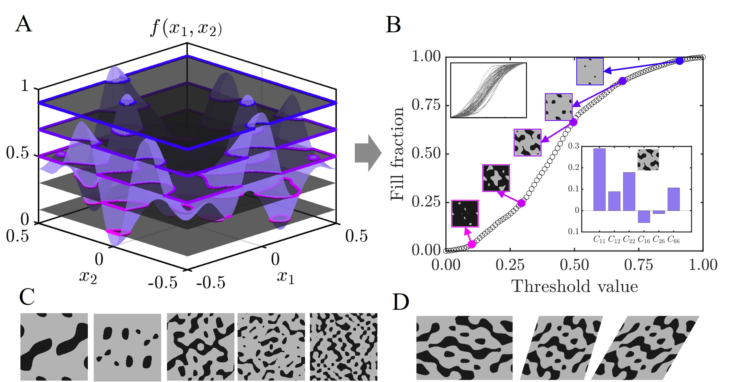
Our goal is to identify the range of effective anisotropic elasticity tensors that can be achieved from periodic single-scale unit-cells composed of two isotropic phases. To accomplish this, we use a pixelated representation for the unit cell geometry parametrization. Exploring all possible combinations of two phases in this pixelated representation is computationally NP-hard111For example, a 100 100 periodic pixelated representation requires the computation of mechanical properties of = unit cells.. Therefore, to sample periodic diverse anisotropic unit cells efficiently with lower degrees of symmetry, we follow an approach introduced in our prior work (Boddapati et al., 2023). This approach is inspired by Cahn’s method of generating Gaussian random fields (Cahn, 1965; Soyarslan et al., 2018; Kumar et al., 2020). Additionally, this method is inspired by the observation that the power spectral density of microstructures in metallic systems tends to be sparse and has peaks highly concentrated at lower spatial frequencies (Zhang and Lu, 2002; Yu et al., 2017), explained in detail in Section A.1 and Fig. 10. We first define a periodic function , as a linear combination of cosine functions:
| (1) |
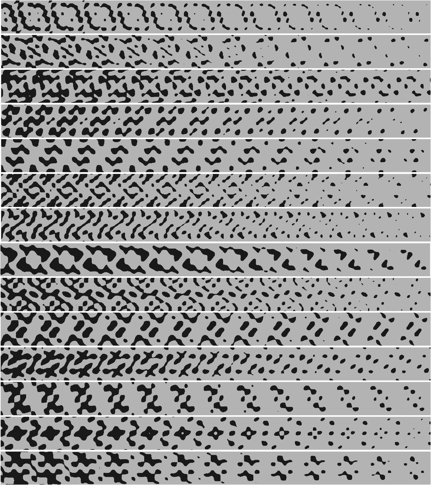
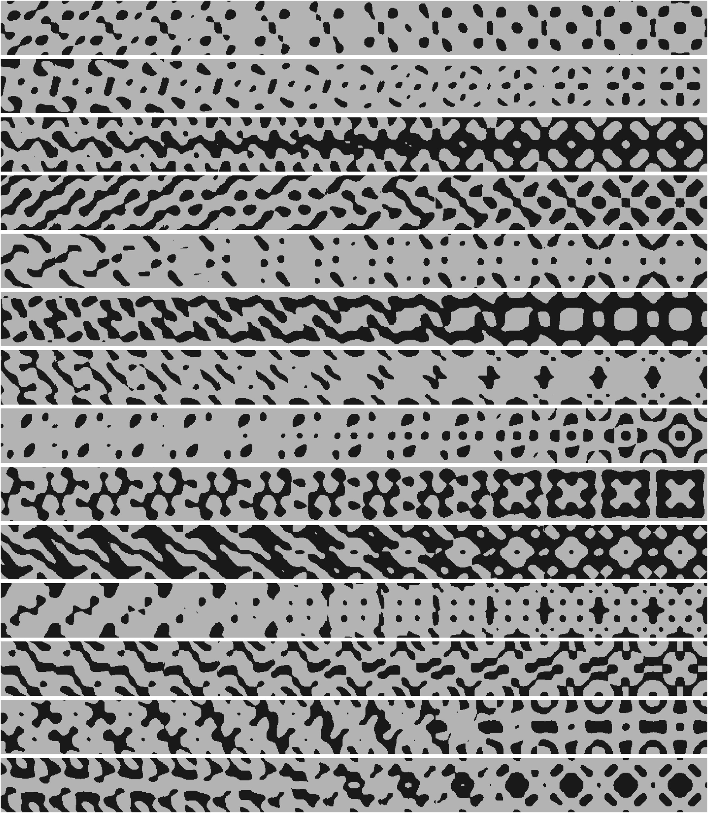
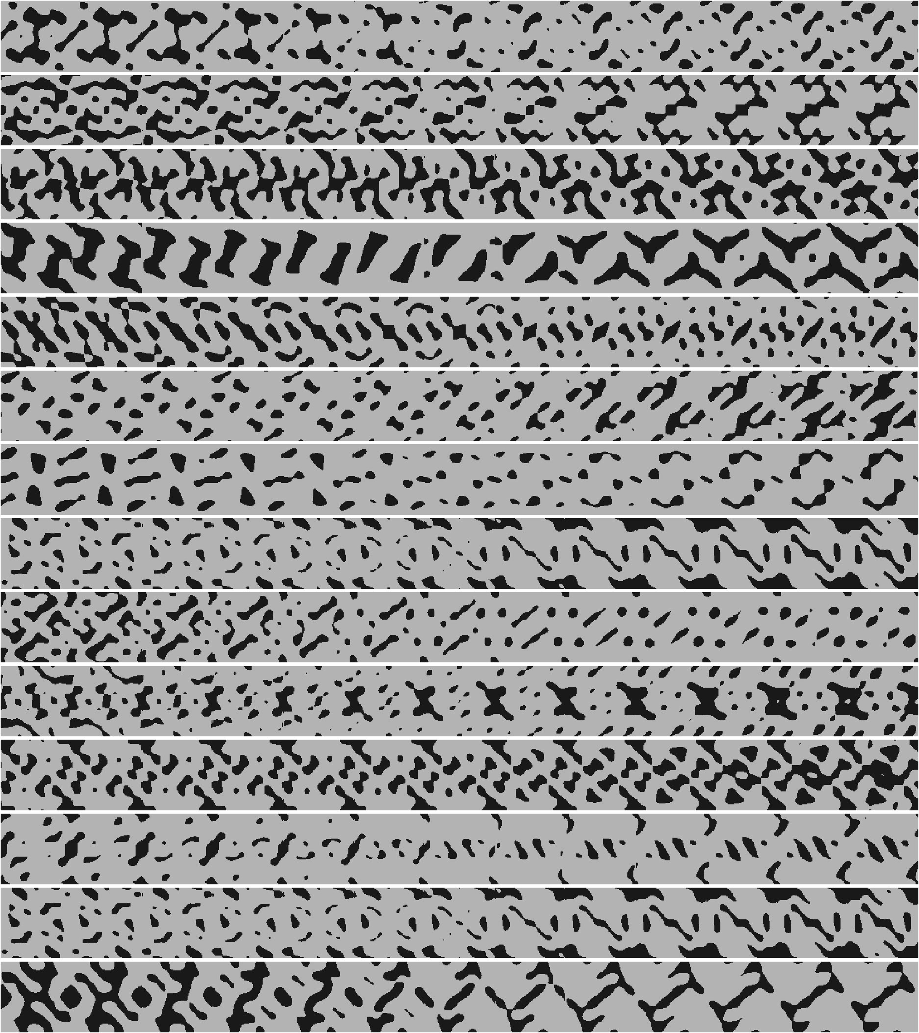
where are spatial frequencies, and are the corresponding cosine function weights Fig. 1A. The function is then thresholded at different values, to generate a family of unit cells, as shown in Fig. 1B.
Several notable observations can be made for this approach. Firstly, the periodicity in the unit cells is ensured by directly selecting cosine functions. Interestingly, choosing between sine and cosine as the fundamental periodic function does not affect the distribution of the resulting properties. By controlling the symmetries in the weights, we can control the symmetries in the unit cell. For instance, if , the result is diagonally symmetric unit cells. Adjusting the pixel density allows us to generate unit cells with arbitrary resolutions as need-based. By increasing the threshold value of the function Eq. 1, the fill fraction of the stiff phase increases monotonically. Each function exhibits a different rate of monotonic increase in the fill fraction, as illustrated in the top inset of Fig. 1B. In this particular work, a few refinements have been made to our previous design approach (Boddapati et al., 2023). The number of spatial modes is a hyperparameter 2+1, with = . In Fig. 1C, the variation of typical feature sizes is shown when the number of spatial modes is varied. Increasing the number of spatial modes leads to smaller feature sizes and increased randomness, resulting in unit cells that tend to be less anisotropic. The shape of the unit cell is also an important factor for achieving anisotropic properties and is a design choice that is often overlooked. By modifying the directions of periodicity in the proposed periodic function definition Eq. 1, we can also generate non-square unit cells as shown in Fig. 1D (explained in detail in Section A.2). Overall, this method allows us to systematically explore a large property space, identify structures that exhibit the desired anisotropic elasticity tensors and is suitable for estimating theoretical bounds on the anisotropic moduli, as discussed in the next section. Further, the coefficients are sampled randomly to generate 2000 different functions and the threshold is varied for 100 increments resulting in a database size of 200000 unit cells as opposed to only 100 unit cells in our previous work (Boddapati et al., 2023).
Each unit cell’s effective material properties are then computed using a numerical homogenization scheme (Francfort and Murat, 1986; Andreassen and Andreasen, 2014). The homogenization scheme is based on length scale separation and follows a two-scale asymptotic expansion of stress equilibrium equation. The resulting effective properties are equivalent in the average energy stored in the unit cell for all possible loading conditions. In computing the effective properties, we fix the pixel resolution at 100. For the gray phase, we use a stiffer material DM8530 ( = 1 GPa, = 0.3) and for black phase, we use a softer material Tango Black ( = 0.7 MPa, = 0.49), representative of materials from commercial multi-material Connex 3D printer. The material properties are experimentally determined following the ASTM D638-14 standard test method. We follow Voigt notation to describe the homogenized constitutive law, assuming plane-strain condition as
| (2) |
where are the six independent elasticity tensor parameters in a given reference frame, are the axial strains, is the shear strain, are the axial stresses, and is the shear stress. The homogenized elastic properties of one of the unit cells, normalized with Young’s modulus of the stiff phase, are shown in Fig. 1B (bottom inset). In order to satisfy thermodynamic stability, parameters along the diagonal of Eq. 2 are always positive, while the parameters on the off-diagonal could be negative. directly relates the axial stress with axial strain , while relates the axial stress with shear strain , and so on. The off-diagonal moduli are also known as shear-normal coupling parameters. We aim to determine the maximum and minimum values a single parameter can reach relative to the others, as discussed in the following section. This understanding helps us evaluate the extent of shear-normal coupling induced by anisotropy.
3 Data visualizations
3.1 Fill fraction plots
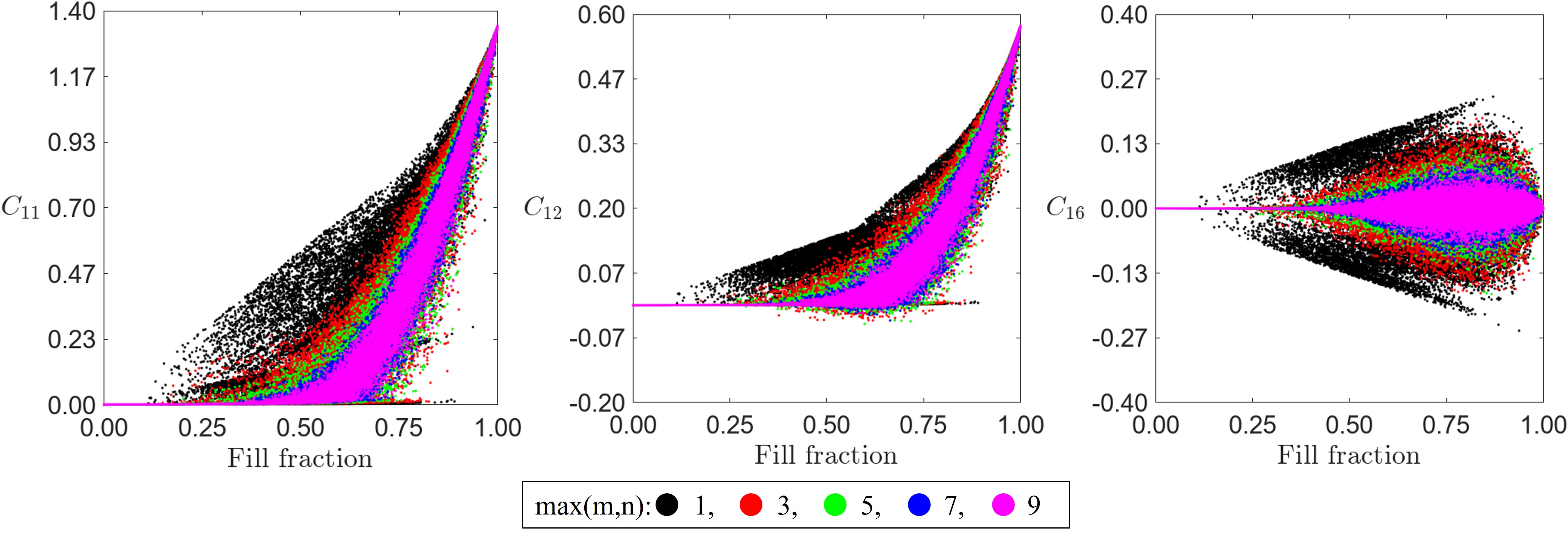
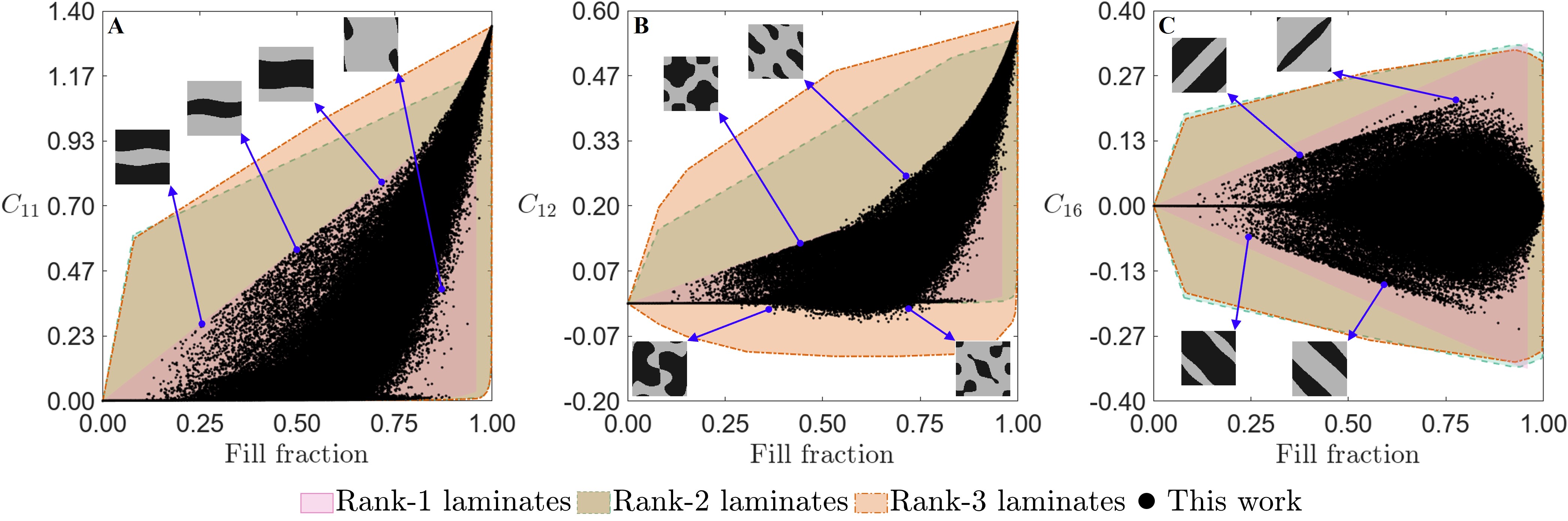
In Fig. 2, the data of material properties is plotted as a function of the fill fraction of the stiff phase. All the parameters are normalized with Young’s Modulus of the stiff phase. Note that , have similar property distribution as that of while property distribution is similar to and hence these parameters are not plotted for brevity. As there are no closed-form expressions for the theoretical bounds on anisotropic moduli, the range of properties achieved by hierarchical laminates upto rank-3 is used as a substitute and indicated in the same plots. Please refer to Section A.3 for a discussion on theoretical bounds and Sections A.4 and 11 for the construction and computation of the effective properties of the hierarchical laminates. First, we observe that in all property plots, rank-2 laminates (shown in green) significantly expand the property range compared to rank-1 laminates (shown in magenta). However, the transition from rank-2 to rank-3 laminates (shown in orange) shows minimal improvement across all moduli except for . For , the negative region is only accessible with rank-3 laminates, and this range shows minimal dependence on the fill fraction beyond 25%. Both rank-2 and rank-3 laminates reduce the strong dependence on achieving higher values for specific moduli, allowing stiffer anisotropic properties beyond linear scaling with a low fraction of the stiff phase. Additionally, hierarchical laminates demonstrate that using anisotropic constituent phases can significantly enhance the range of achievable properties in single-scale two-phase composites.
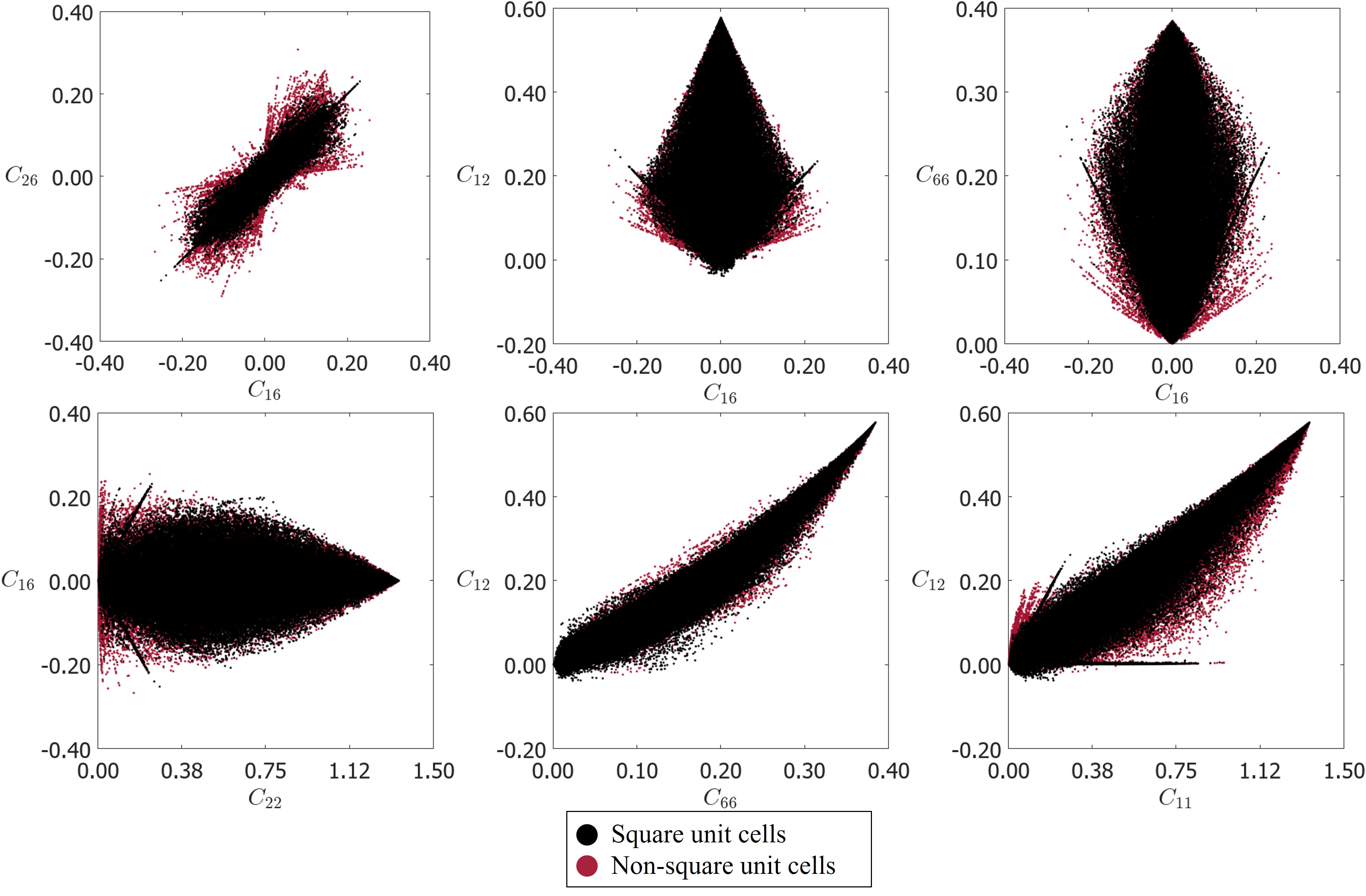
Our database consisted of unit cells achieving the bounds predicted by rank-1 laminates, specifically in the fill fraction ranging between 30% - 80%. To understand the effect of spatial frequencies, the same plots are plotted in different colors with data constructed from adding a specific number of spatial frequencies (Fig. S1). It is observed that adding higher spatial modes doesn’t necessarily increase the reach in the property space. In fact, adding higher spatial modes is detrimental to producing anisotropic structures beyond spatial modes of order 3. While square unit cells were sufficient to explore the extremes of the diagonal moduli, the range of the off-diagonal moduli is enhanced with the use of non-square unit cells (Fig. S2). For , the structures at the upper bound are laminate-like structures aligned along the direction, while those at the lower bound are laminates aligned along the . For , the unit cells at the upper and lower bounds are non-laminate-like. In the negative , the discovered unit cells do not approach the bounds of rank-3 laminates and feature chiral patterns and/or orthogonally aligned thin features. For , the upper bound unit cells are skew laminates tilted towards right, while those at the lower (negative) bound are the same skew laminates, but flipped.
Hierarchical architectures plays a significant role in structural integrity and functionality across systems of various length scales (e.g. spider silk) (Nepal et al., 2023). This hierarchy is often present in non-rectangular coordinate systems. For example, wire ropes used in structural engineering contain helical strands arranged in a hierarchical manner, enhancing efficient load transfer and their strength by distributing tensile forces uniformly throughout the cross-section, regardless of the bending direction (Feyrer, 2007). In biological systems, spinal discs, which are annular cylinders surrounding the spine in the vertebrae, provide shock absorption, support, and flexibility to the spine. Their load-bearing protein, collagen, is distributed in a multi-layered laminar fashion (Tavakoli and Costi, 2018). Similarly, the tympanic membrane of the human ear, which is responsible for efficient sound transmission and protecting the delicate structures within the ear, is conical in shape and features collagen structured in a trilaminar fashion with radial and circumferential patterns (Volandri et al., 2011). These observations along with findings from our work further emphasize the importance of incorporating hierarchical designs to enhance the design capabilities.
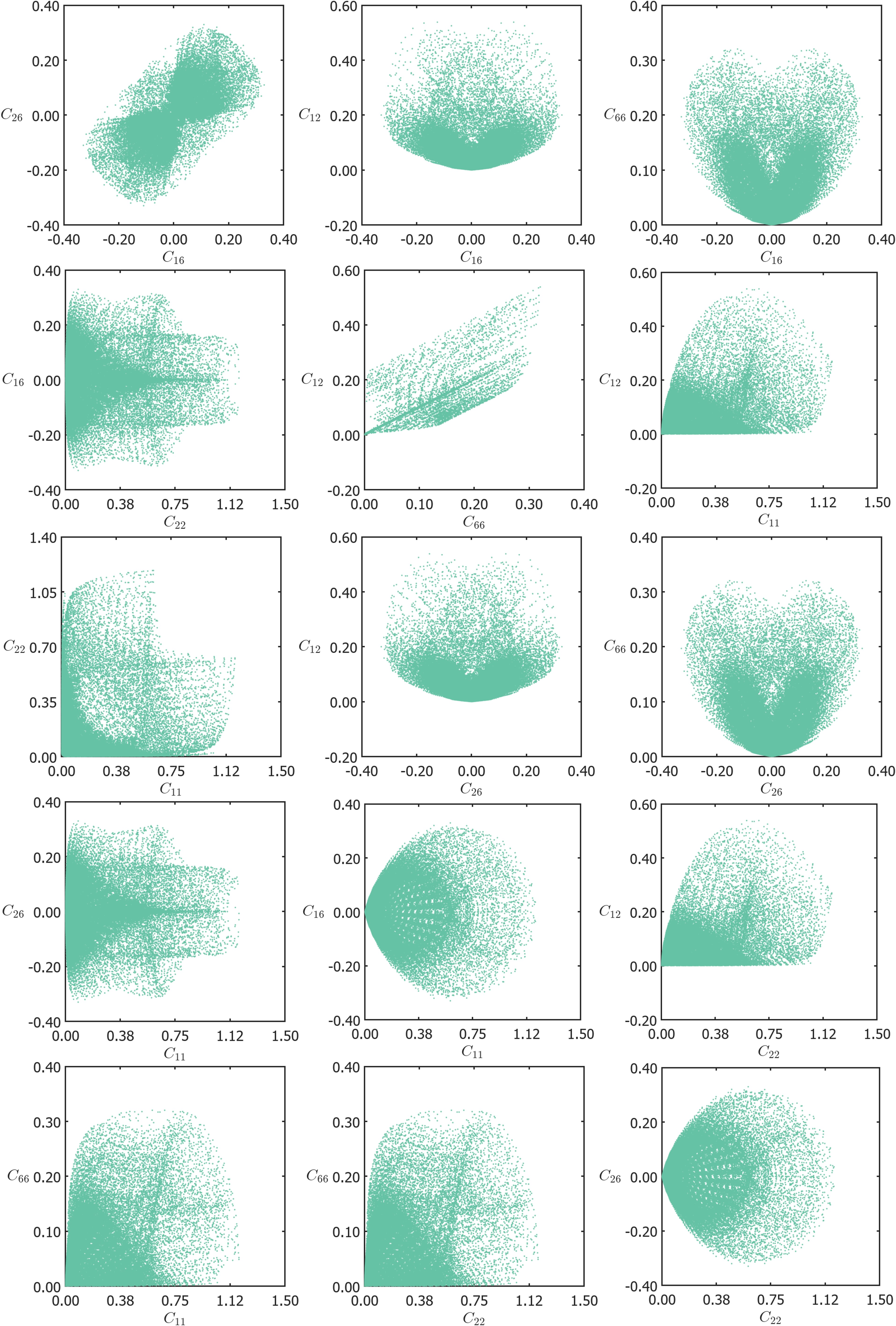
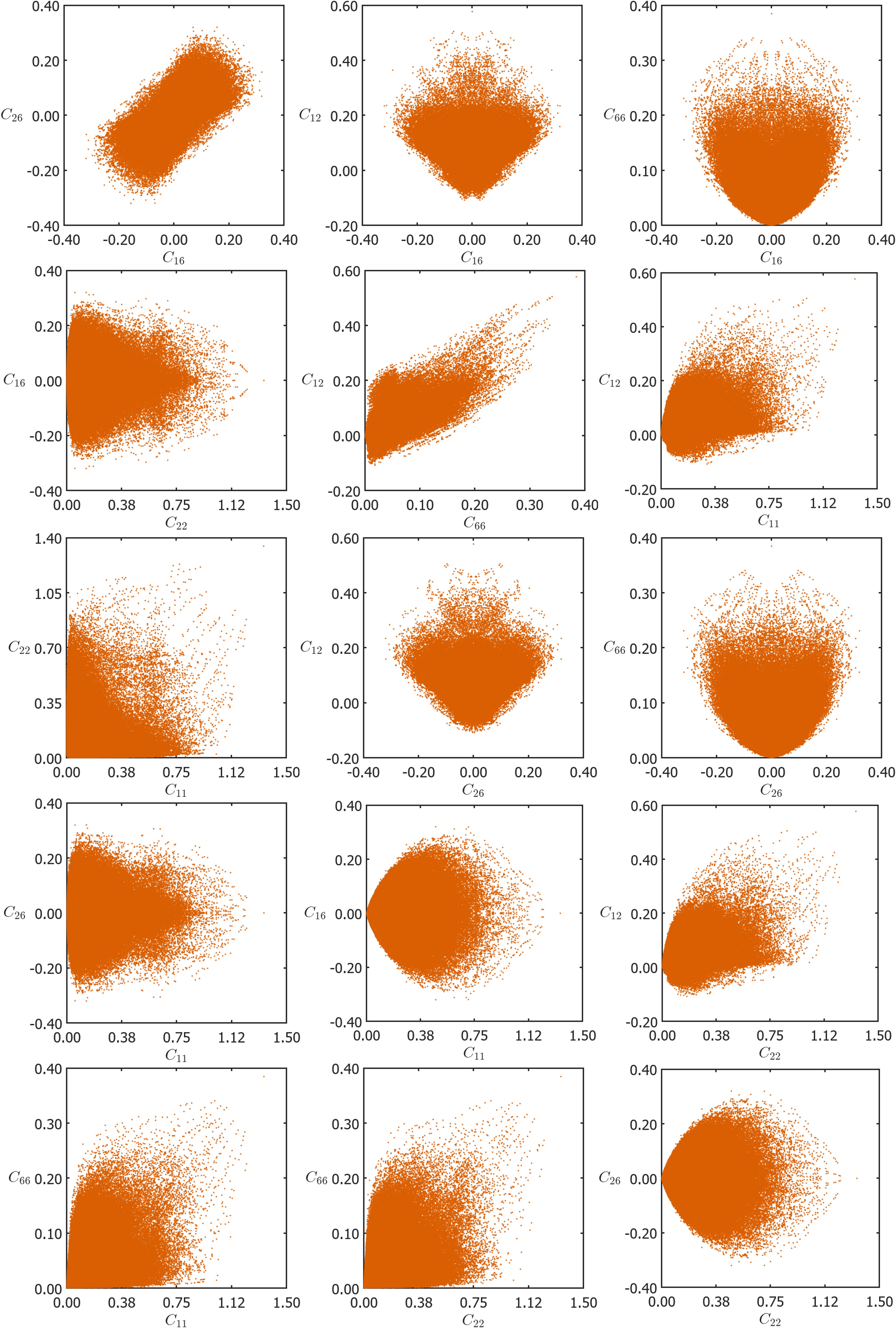
3.2 Pair property plots
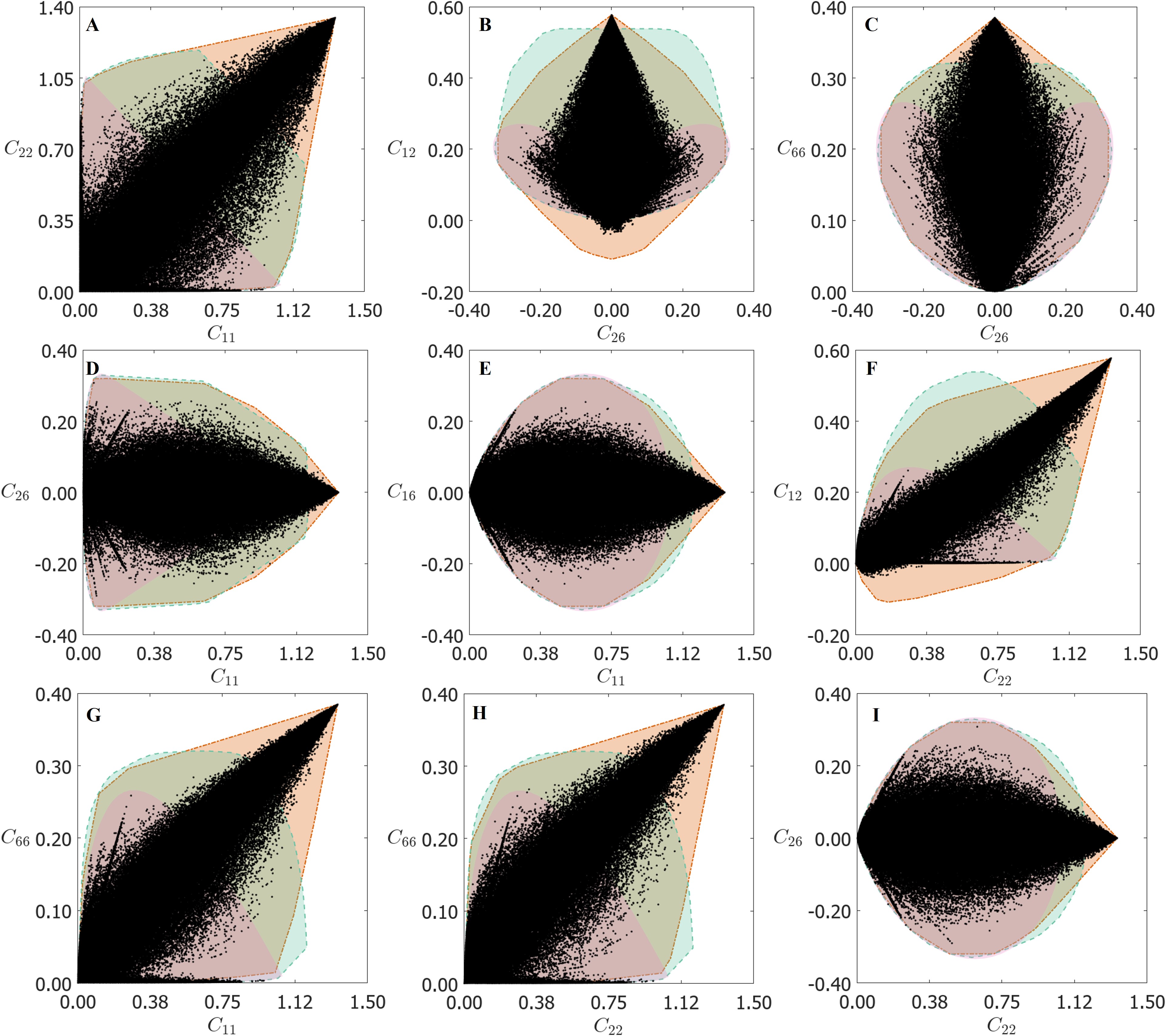
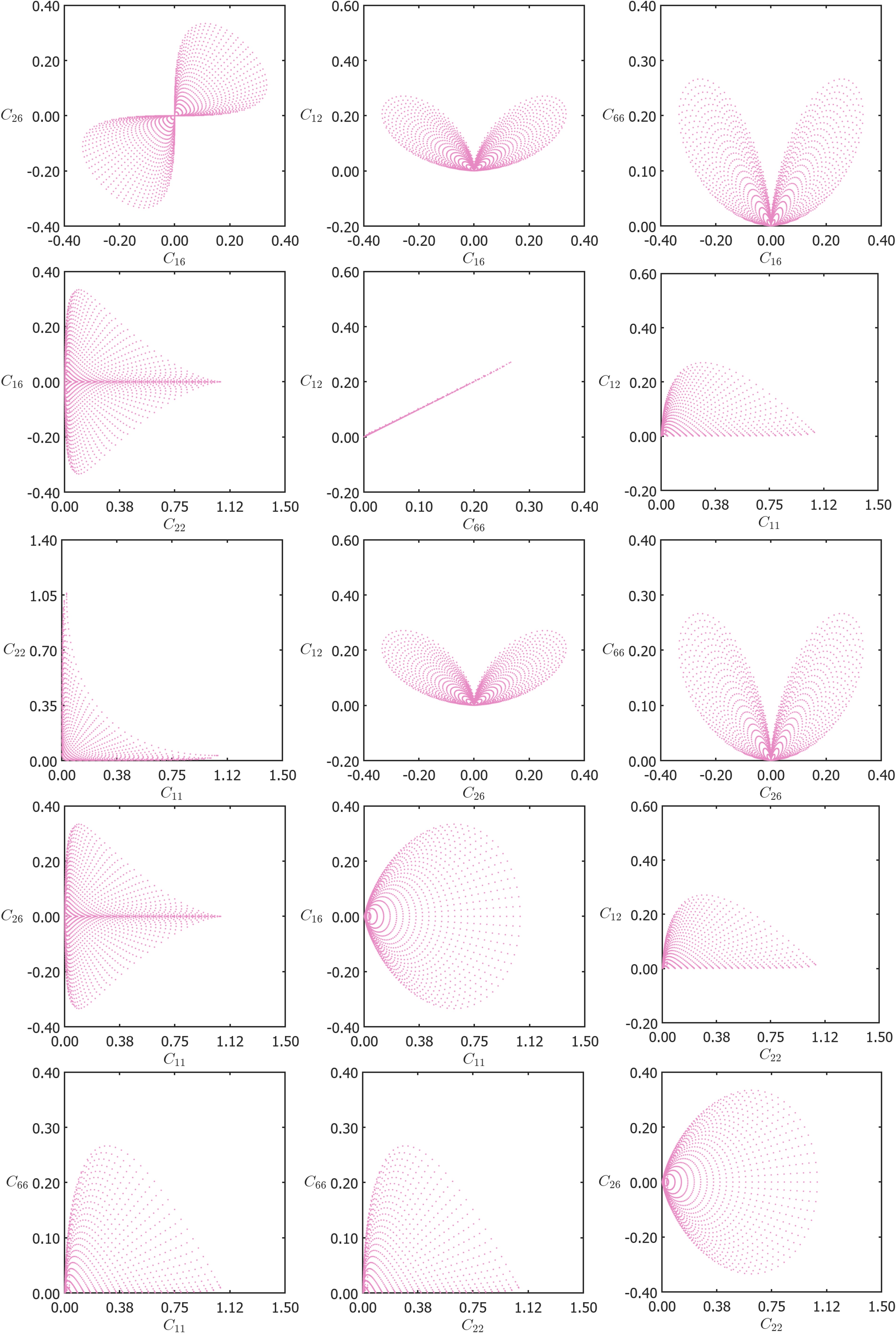
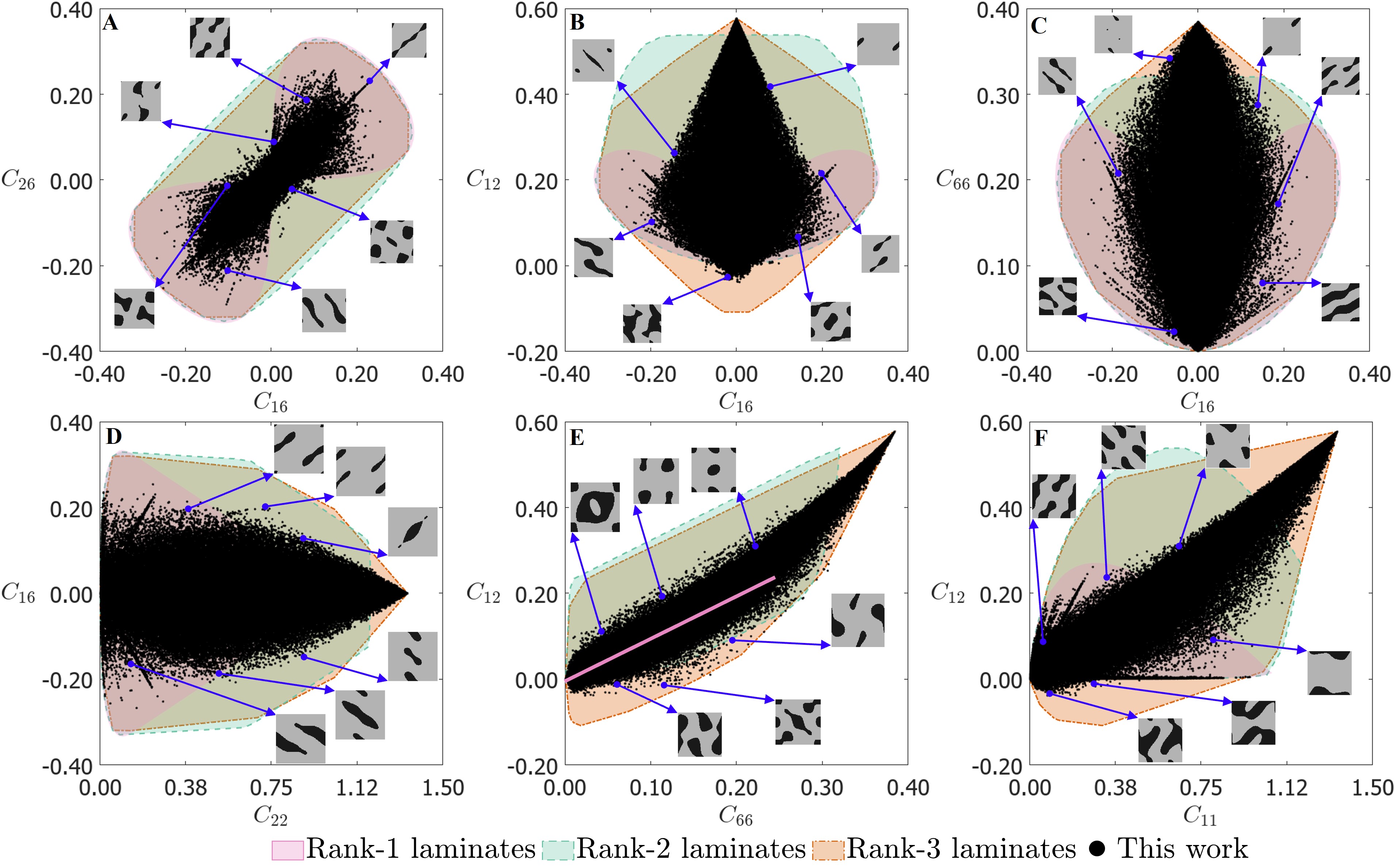
Often, multiple components of the elasticity tensor contribute to the overall mechanical behavior. Therefore, we also examine the pair property plots. For a total of 6 material parameters, there are a total of = 15 distinct pair property plots. However, due to the symmetry nature of the property plots, it is sufficient to consider only a subset of the plots. For example, the property plot of vs would be the same as vs . As the goal of this paper is to identify anisotropic structure-property relations, specifically shear-normal coupling, the property plots associated with the off-diagonal parameters of the elasticity tensor are discussed in detail. Therefore, the property plots corresponding to vs. , vs. , vs. , . are shown in Fig. 3. Please refer to Fig. S3 for the rest of the pair-property plots. In the same plots, as discussed earlier, the range of properties achieved by hierarchical laminates are used as a substitute for theoretical bounds (which are plotted separately in Figs. S4, S5 and S6 to indicate their distinction).
In the property plot of vs. shown in Fig. 3A, we observe that there is a strong correlation along the line inclined at 45∘. This means for many of the unit cells, both and have the same sign. Hierarchical laminates uncorrelated this behavior and achieved unit cells with opposing signs for and . The unit cells identified on the boundary of this property space resemble rank-1 laminates. As discussed in (Forte and Vianello, 2014), and are components of the invariants of the elasticity tensor under coordinate transformation. Each of these sums signifies a different contribution to the stored elastic energy (see Eqs. S11 and S12 in Appendix S-I). In the property plots of vs. and vs. shown in Fig. 3E-F, there are generally very few data points with a negative value of , especially at high values of . Again, the negative region for is only accessible with rank-3 laminates. The combination , known as the bulk modulus, is an invariant. This imposes a restriction on the negative bound of to ensure that remains positive. The parameter is invariant under coordinate transformation. Therefore, vs. plot for rank-1 laminates is strictly a single linear line. vs. plot for rank-2 and rank-3 laminates is composed of several such lines with different slopes, which is clearly observed in Fig. S5.
To validate the effective homogenized behavior of unit cells, we conducted experiments on finite tessellations of four different unit cells in a separate study (Boddapati et al., 2023). In this study, we successfully identified all the anisotropic moduli including shear-normal coupling parameters. The results showed that at least 10 repeated unit cells in the tessellated structure are required to satisfy homogenization conditions.
4 Functionally graded structures
4.1 Method of generation of functionally graded structures
Functionally graded structures have been shown to exhibit unique mechanical behavior such as avoiding shear-banding (Chen et al., 2023; Tian et al., 2024) and, mimicking bone stiffness (Kumar et al., 2020). To generate such structures, the parametrization associated with the structure such as truss thickness is often adjusted (Panesar et al., 2018; Sanders et al., 2021; Wu et al., 2023). Therefore, these approaches are particularly effective in controlling the isotropic Young’s Modulus, relative density, and to some extent, the degree of orthotropic elasticity (Li et al., 2018; Garner et al., 2019). However, achieving smooth spatial gradients in the anisotropic mechanical properties while ensuring the connectivity of adjacent unit cells is challenging. Here, we illustrate the construction of functionally graded anisotropic structures with seamless transition between unit cells with distinct patterns.
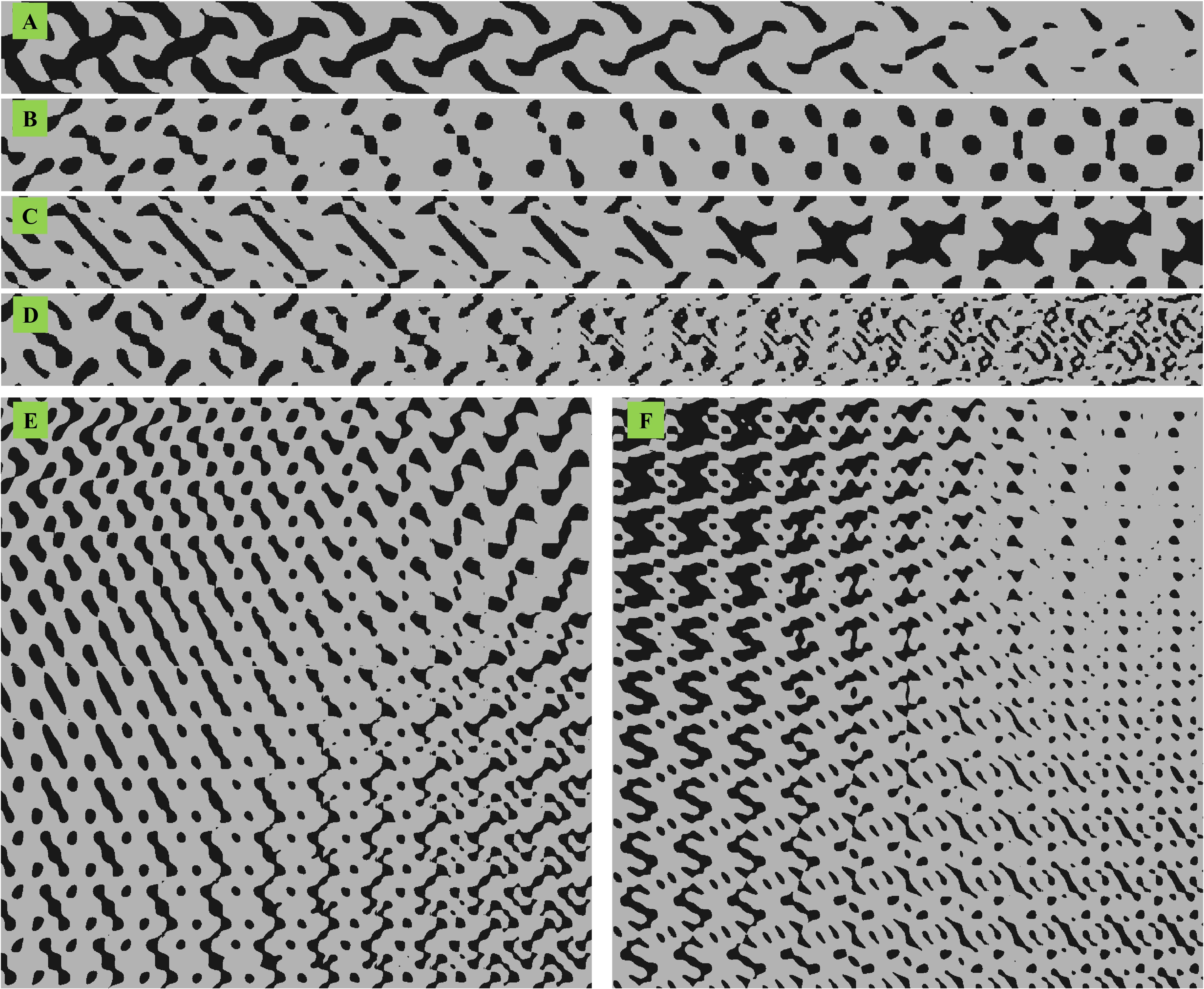
For this purpose, we use the proposed functional representation used to generate unit cells in Section 2. We introduce the local variables as well as the global variables . The global variables are defined only on a coarser grid, while the local variables are defined on a finer grid. In a graded structure with unit cells, with , the global variables change at discrete locations given by the unit cell centers, while the local variables change at each pixel location within the unit cell at a given . The function that is required to generate the graded structure is thus given by
| (3a) | ||||
| (3b) | ||||
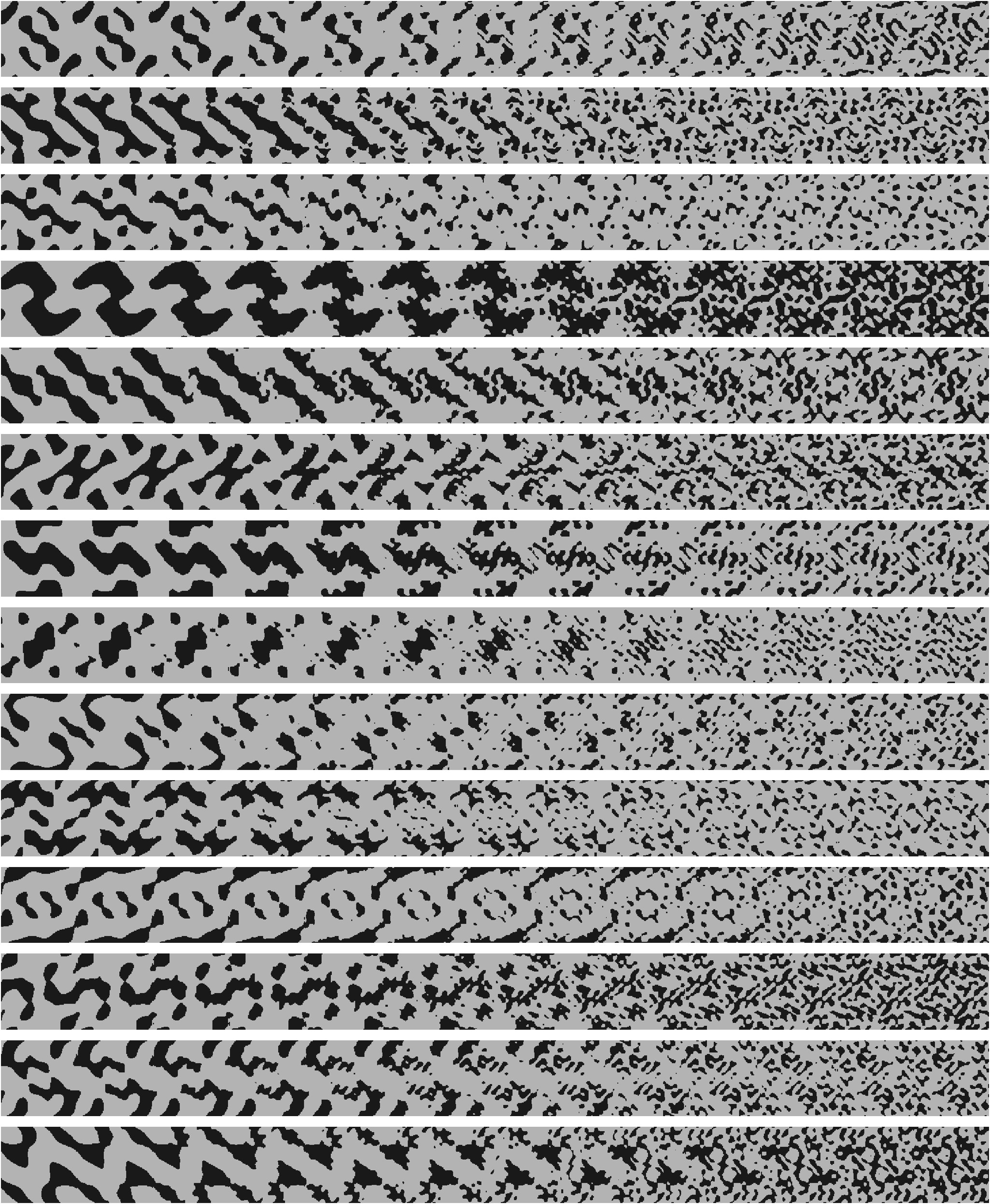
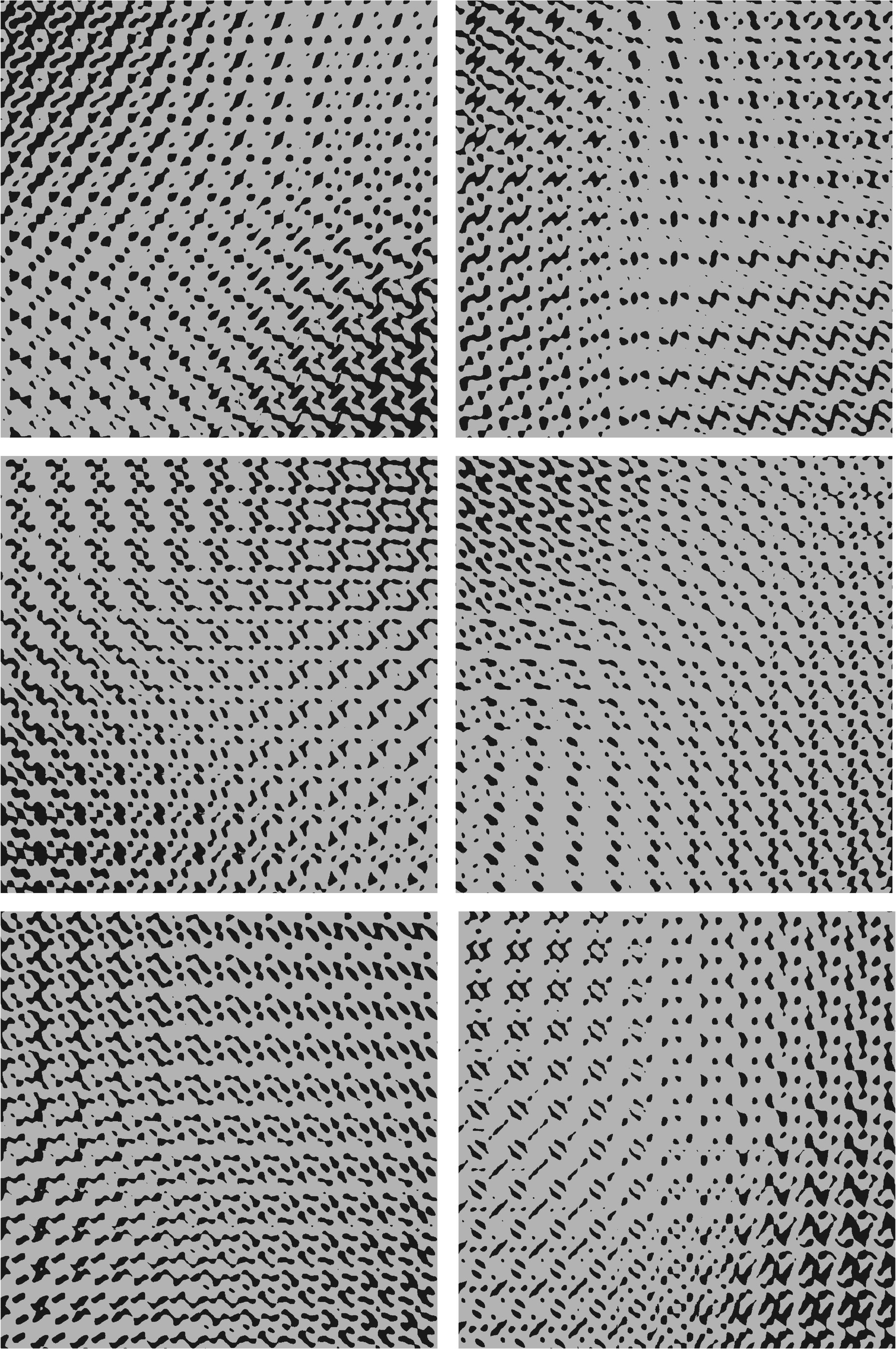
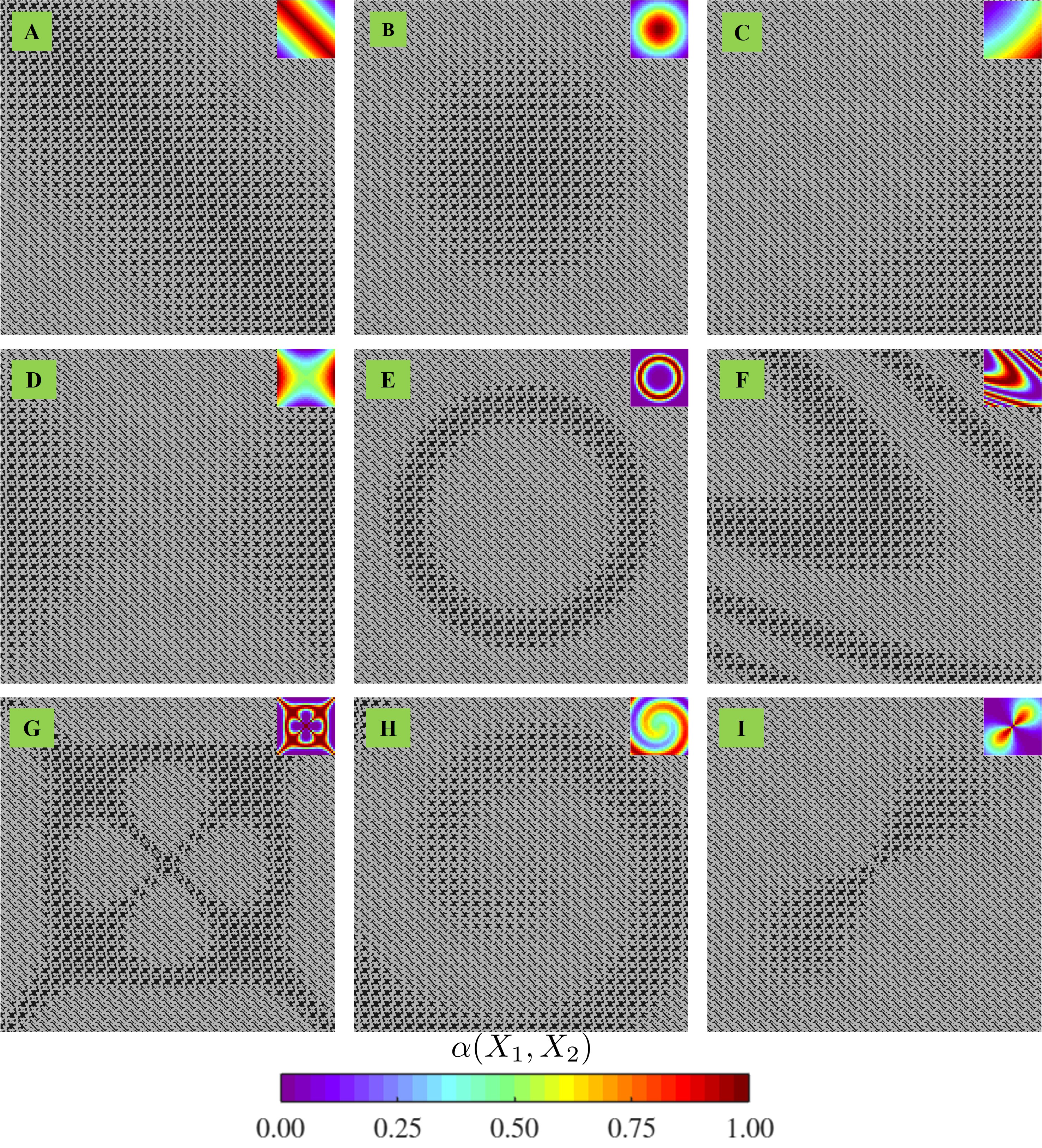
where , are weighing parameters such that . An increase in signifies the increase in the contribution of second function in the interpolated unit cell. The threshold to generate graded structure from the function is subsequently set by a bilinear interpolation determined by the thresholds set for the unit cells at the ends. This method allows for independent control of several functional gradients, such as porosity, anisotropic moduli, and symmetry. In Fig. 4A-D, various functionally graded structures are shown with different gradients along the -axis using Eq. 3a while maintaining periodicity along the -axis. Fig. 4E-F shows the bilinear interpolation between four unit cells with different anisotropic behavior at four corners of the boundary. By using nonlinearly interpolated weighing parameters, various graded designs such as radial, elliptical, spiral, star, and many more can be created. Fig. 5 illustrates the designs interpolated non-linearly using the unit cells depicted in Fig. 4C. More examples on the graded designs are added to the supplementary information (see Fig. S7, Fig. S8, Fig. S9, Fig. S10, Fig. S11). In the next section, we investigate the mechanical behavior in two gradient structures with nonlinear interpolations in eliciting atypical mechanical behavior.
4.2 Mechanical behavior of graded structures
4.2.1 Selective elastic energy localization
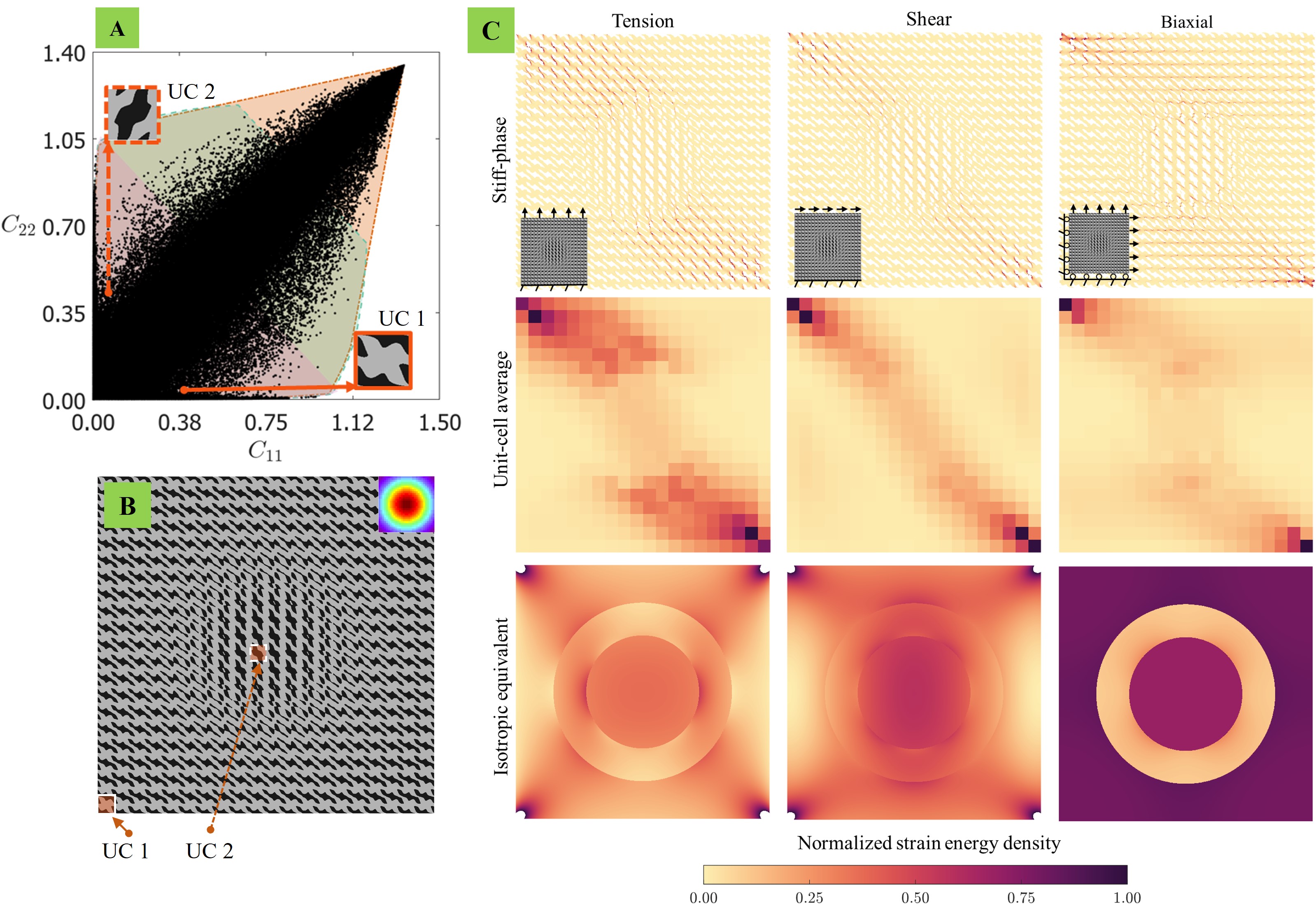
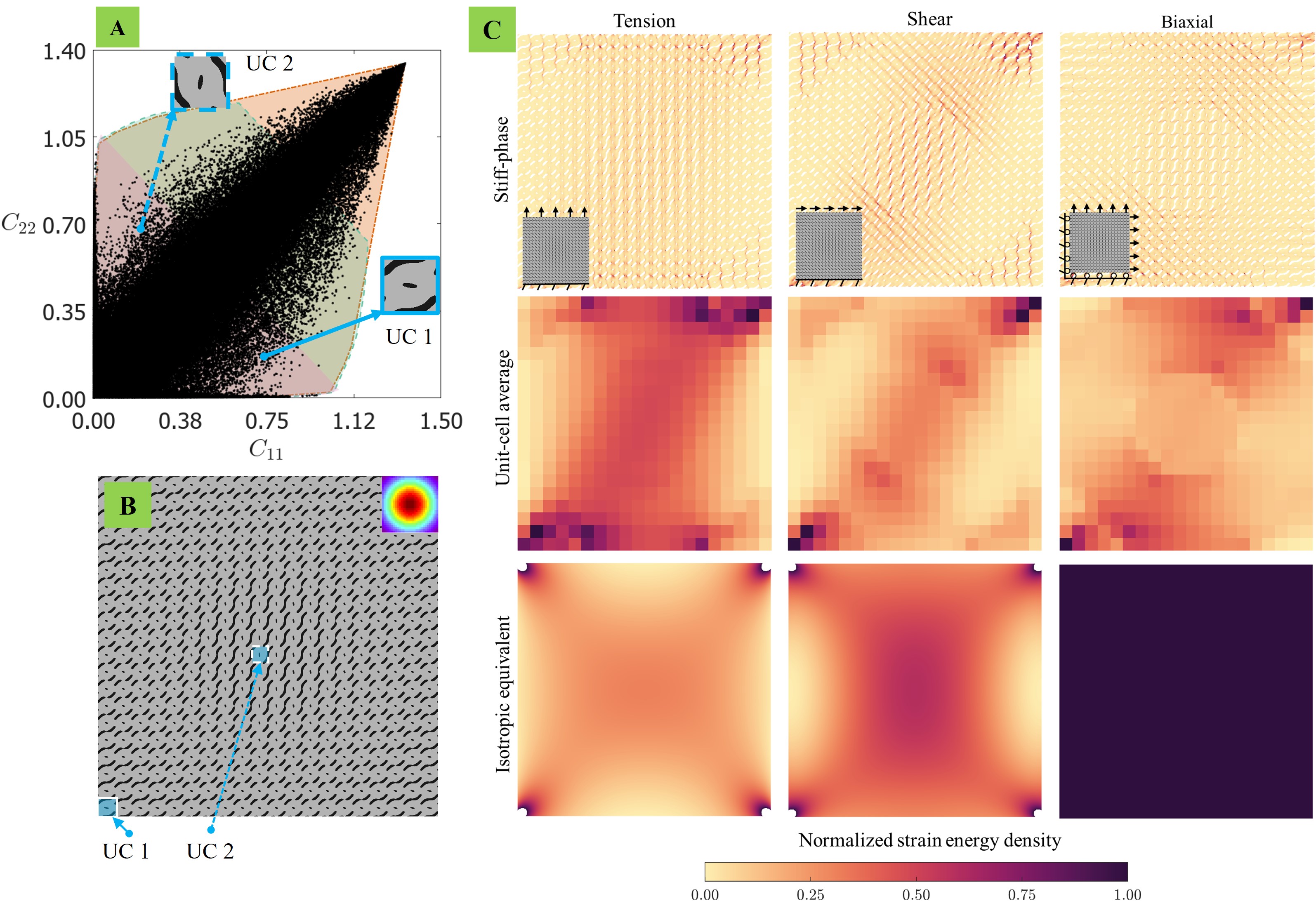
Energy localization refers to the phenomenon where strain energy in a material or structure is concentrated in specific regions. Energy localization finds use in applications such as mechanical sensing (Lee et al., 2023), and energy harvesting (Lee et al., 2022). Here we show that graded structures with anisotropic unit cells achieve selective energy localization, i.e., different localization behavior under different loading conditions. we achieve this using functionally graded structures with strategically selected unit cells in a radially interpolated design. The unit cells are chosen such that unit cell #1 at the boundary is obtained by a 90∘ rotation of the unit cell #2 at the interior. The fill fraction of the stiff phase of both the unit cells is 80% respectively. Therefore, this choice makes most of the unit cells in the 20 20 interpolated structure also have uniform fill fractions close to 80%. A uniform fill fraction is selected in the graded design to isolate the impact of differences in stiffness parameters from unit cells that may also be affected by varying fill fractions. The (vectorized) stiffness tensor of the unit cell #1 at the boundary is [0.698 0.131 0.221 0.138 0.095 0.150]T222In the vectorized format, the stiffness components are ordered as . Therefore, the (vectorized) stiffness tensor of the unit cell #2 is [0.221 0.131 0.698 0.095 0.138 0.150]T.
We subject this graded structure to three different loading conditions namely, tension along direction, simple shear along applied on the top edge towards direction, and a biaxial tensile loading by prescribing a displacement of 1.5 mm. In Fig. 6, the elastic energy density stored in the structure, defined as is obtained from finite element analysis (FEA). Here we have used the Einstein summation convention, assuming summation over repeated indices, and the double dot “:” indicates a double contraction of indices. The energy density is plotted first just in the stiff phase, then as areal (volumetric) average at each unit cell while including both the phases. The energy distribution is then compared with an effective isotropic medium. The isotropic equivalent is calculated by replacing unit cell with a material whose bulk and shear moduli are that of Hashin-Shtrikman upper bound for the corresponding fill fraction. We observe that under tensile loading the energy distribution becomes significantly localized in a few unit cells in the central region. In contrast, for the simple-shear boundary condition, the energy is localized in the diagonal region. For the biaxial loading condition, energy is distributed in the region exterior to the center 333It should be noted that the maximum value of the energy density for three loading cases is different. We are interested in the distribution over the exact values of the energy density.. The unit cell #2 in the interior has a higher compared to the unit cell #1 at the boundary. Therefore, under tensile loading along direction, the interior region acts stiffer compared to the exterior region. This geometric frustration results in increased stresses in the interior region. Subsequently, the energy is significantly localized in the center. As for shear loading, the shear-normal coupling in the unit cells distributes the stresses along the identified diagonal region. In the biaxial loading condition, although the fill fraction of all the unit cells is almost same, the interior region is under relatively lower stresses. If both the unit cells were to be isotropic, this distinctive energy localization is not seen. The gradient structures can thus localize energy which can be programmed to have a specific failure mode and/or localize stresses and strains in a preprogrammed location. We further demonstrate the general applicability of this effect when tested with two other unit cells (see Fig. S12).
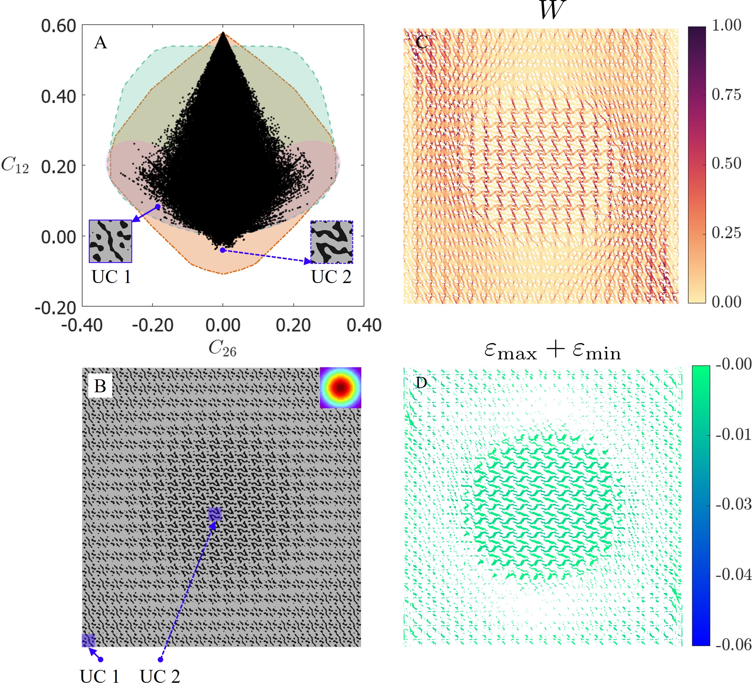
While plotting the energy density distribution provides valuable insights, localization occurs due to all stress and strain components. To delve deeper into this, we select unit cells where the interior region contains those with negative values for , while the exterior region contains positive values for , as depicted in Fig. 7. The (vectorized) stiffness tensor of the unit cell #1 (UC1) at the boundary is [0.134 0.082 0.370 -0.050 -0.120 0.107]T. Similarly, the (vectorized) stiffness tensor of the unit cell #2 (UC2) in the interior is [0.171 -0.009 0.096 0.001 -0.017 0.248]T. The fill fraction of the stiff phase for the unit cells is [73.7%, 59.2%] respectively. The behavior of this design under tensile loading is studied. In this specific scenario, we observe that unit cells in the interior exhibit chiral characteristics, resulting in lateral expansion akin to auxetic behavior. Conversely, unit cells in the exterior, lacking chirality, contract laterally under tensile loading. This geometric mismatch compels interior unit cells to experience compression despite their inherent tendency to expand. Consequently, the region with softer-like properties bears greater stresses and strains, leading to a concentration of energy in the center.
4.2.2 Non-affine deformations
Non-affine deformations refer to deformations of a material where the local strain or displacement of the material points does not follow the global deformation applied to the material. Often soft materials such as polymers, biological tissues, and granular systems exhibit non-affine deformations due to the rearrangement of molecules, particles and/or grains (Rubinstein and Panyukov, 1997; Ellenbroek et al., 2009). Such non-affine deformations play a crucial role in energy dissipation.
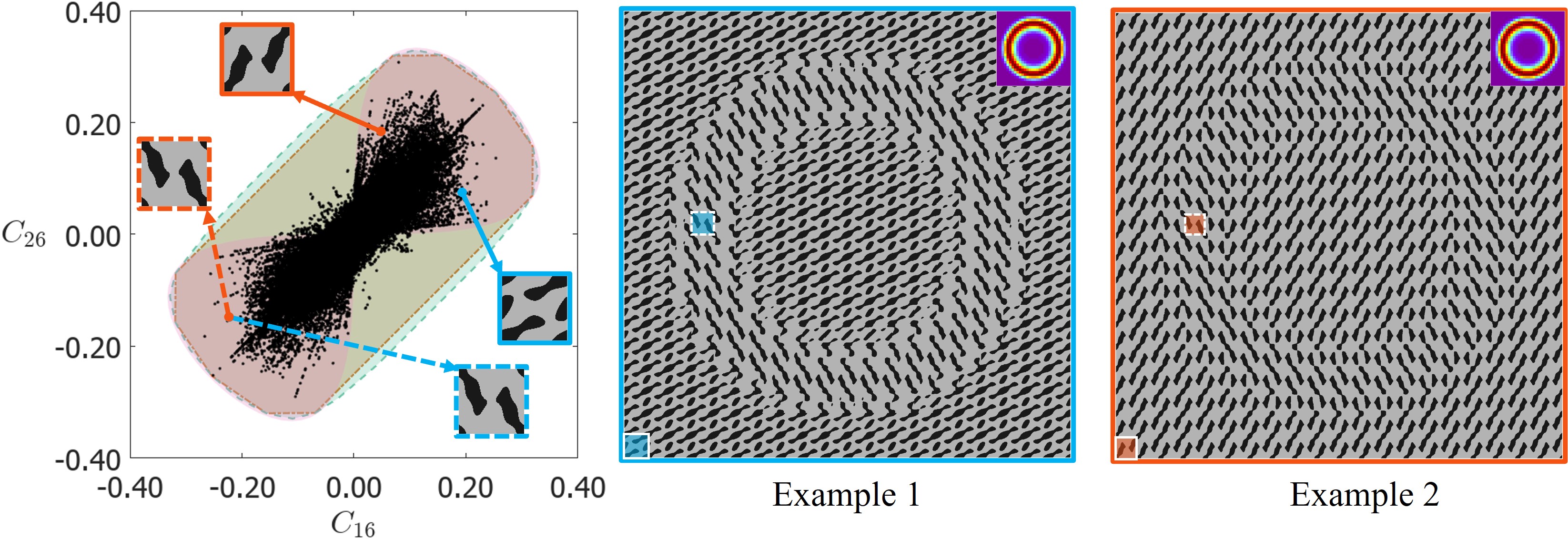
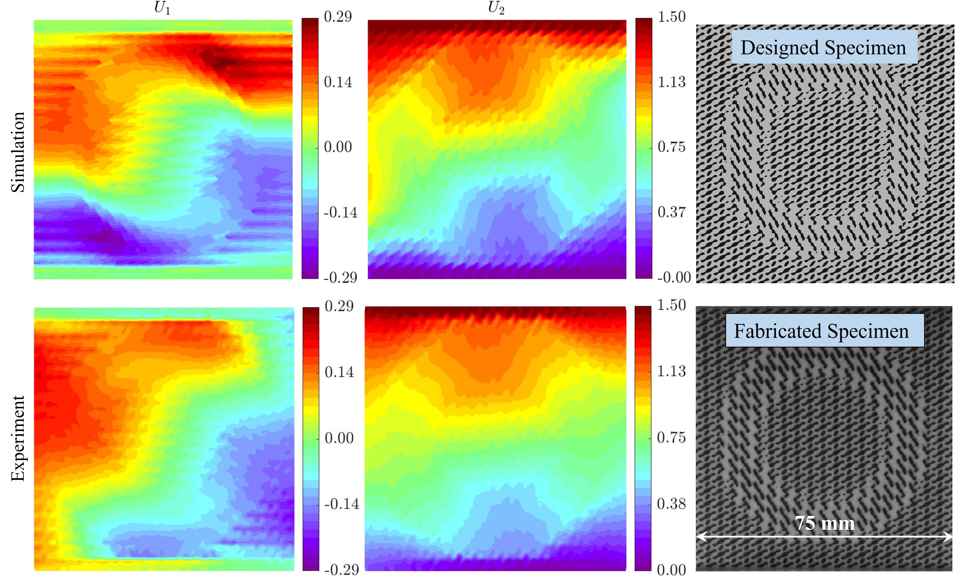
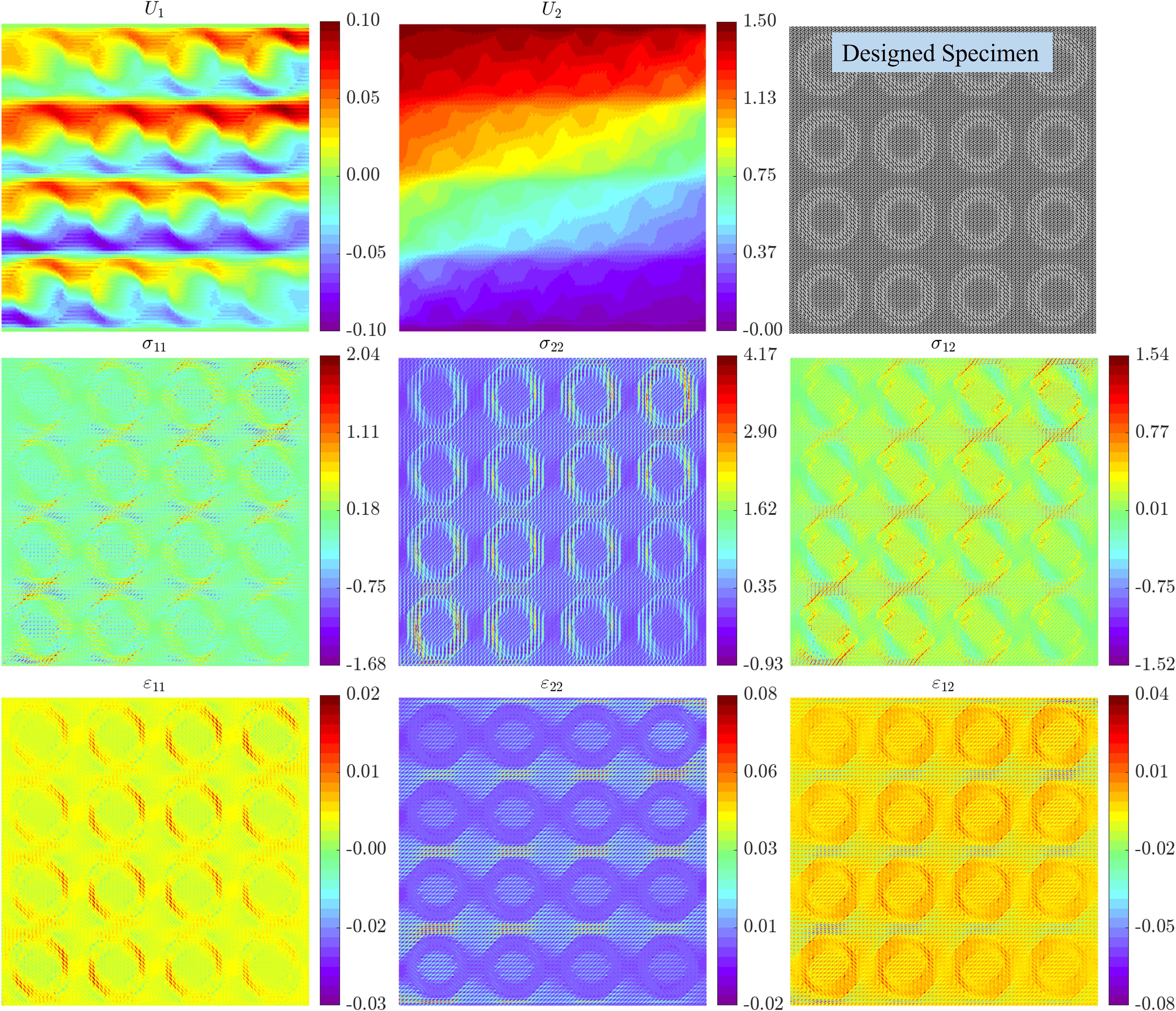
Here, we present an example of inducing non-affine deformations in metamaterials on a global scale by utilizing functionally graded structures with strategically selected unit cells. The two unit cells selected for interpolation are chosen such that their off-diagonal shear-normal coupling moduli are opposite in sign while the other moduli and fill fraction are comparably close. We then create an annular interpolated structure as discussed in Fig. 5C with 20 unit cells along each axis. Please refer to Fig. S13 for more details on the selection of unit cells and their interpolation. The (vectorized) stiffness tensor of the unit cell in the boundary upon normalization is [0.374, 0.101, 0.108, 0.134, 0.066, 0.110]T. The (vectorized) stiffness tensor of the unit cell in the annular region upon normalization is [0.115, 0.121, 0.494, -0.084, -0.147, 0.138]T. The fill fraction of the stiff phase for the unit cells is [62.7%, 69.5%] respectively. As a result, most of the unit cells in the 20 x 20 interpolated structure have fill fractions close to 65%.
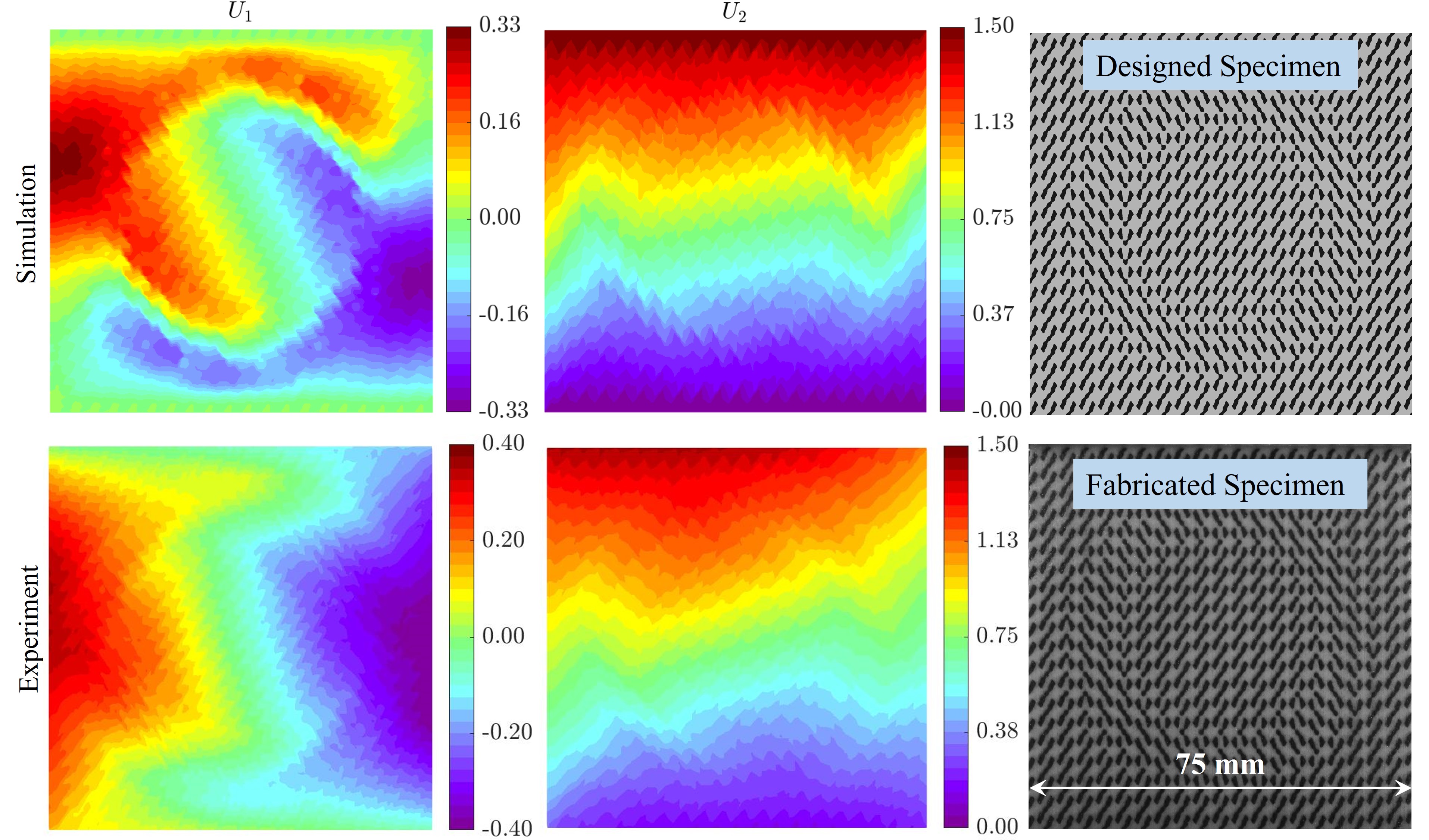
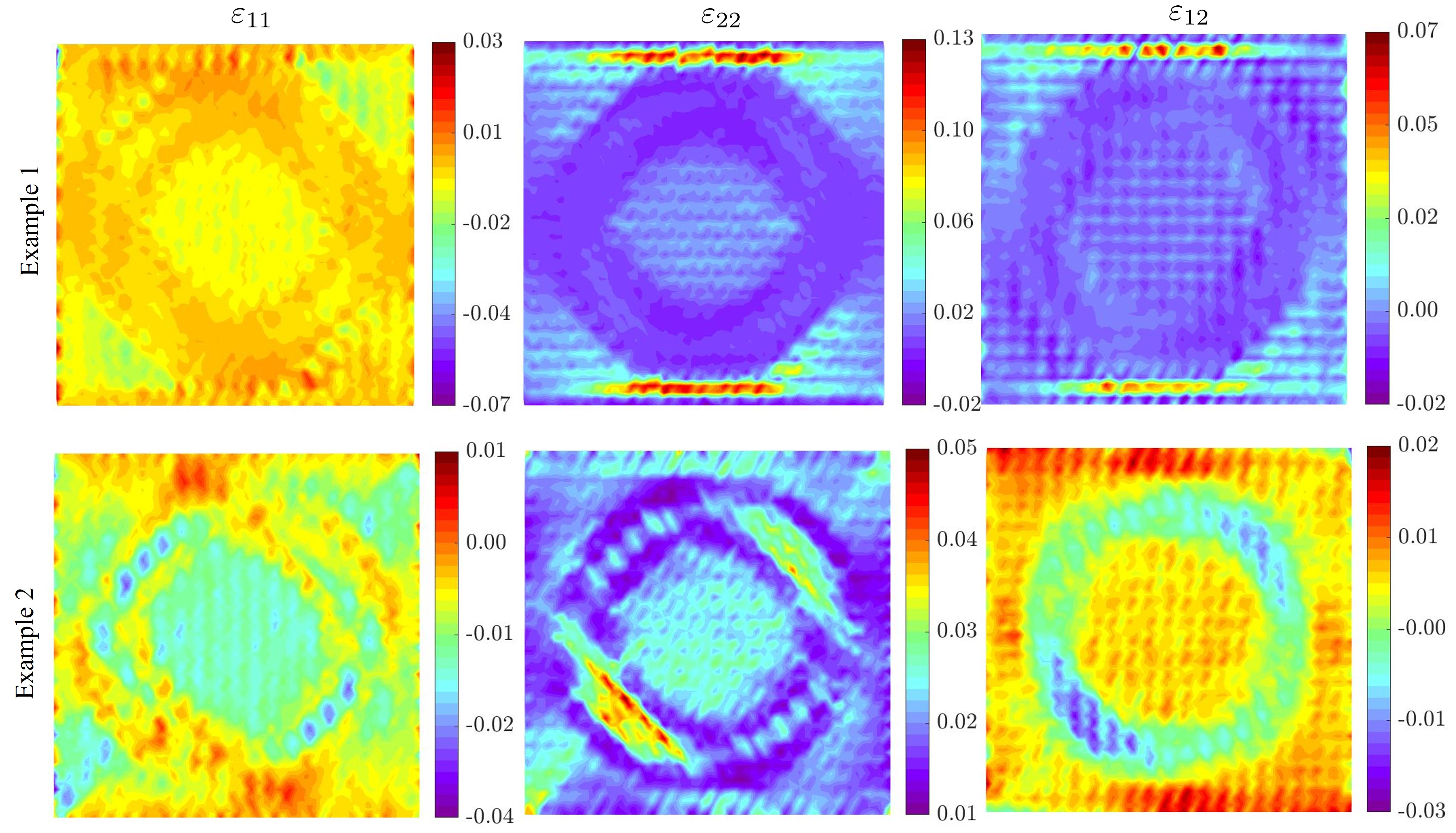
This structure is subjected to a tensile loading along direction by prescribing a displacement of 1.5 mm at the top end. In Fig. 8, the numerical simulations (assuming linear elasticity) reveal that the horizontal displacements exhibit a rotation-like characteristic under this tensile loading. We further experimentally corroborate the same behavior using full-field measurements obtained using digital image correlation (DIC). More details on the experimental procedure can be found in Appendix S-II. This non-affine deformation behavior seems to arise from the incompatibilities in the off-diagonal shear-normal coupling moduli () between the two selected unit cells. The unit cells with positive shear-normal coupling moduli have a preferential direction to shear under tension, which is opposite to the preferential direction of the unit cells with negative shear-normal coupling moduli. Therefore this incompatibility in the preferential direction to shear under tension creates internal torque and directs the annular region to rotate while extending in the direction. In Fig. S14, we demonstrate that the observed behavior can also be seen in other pairs of unit cells with opposing shear-normal coupling moduli. Additionally, experimentally measured strains are presented for this example in Fig. S15, indicating the localization of strain around the annular region.
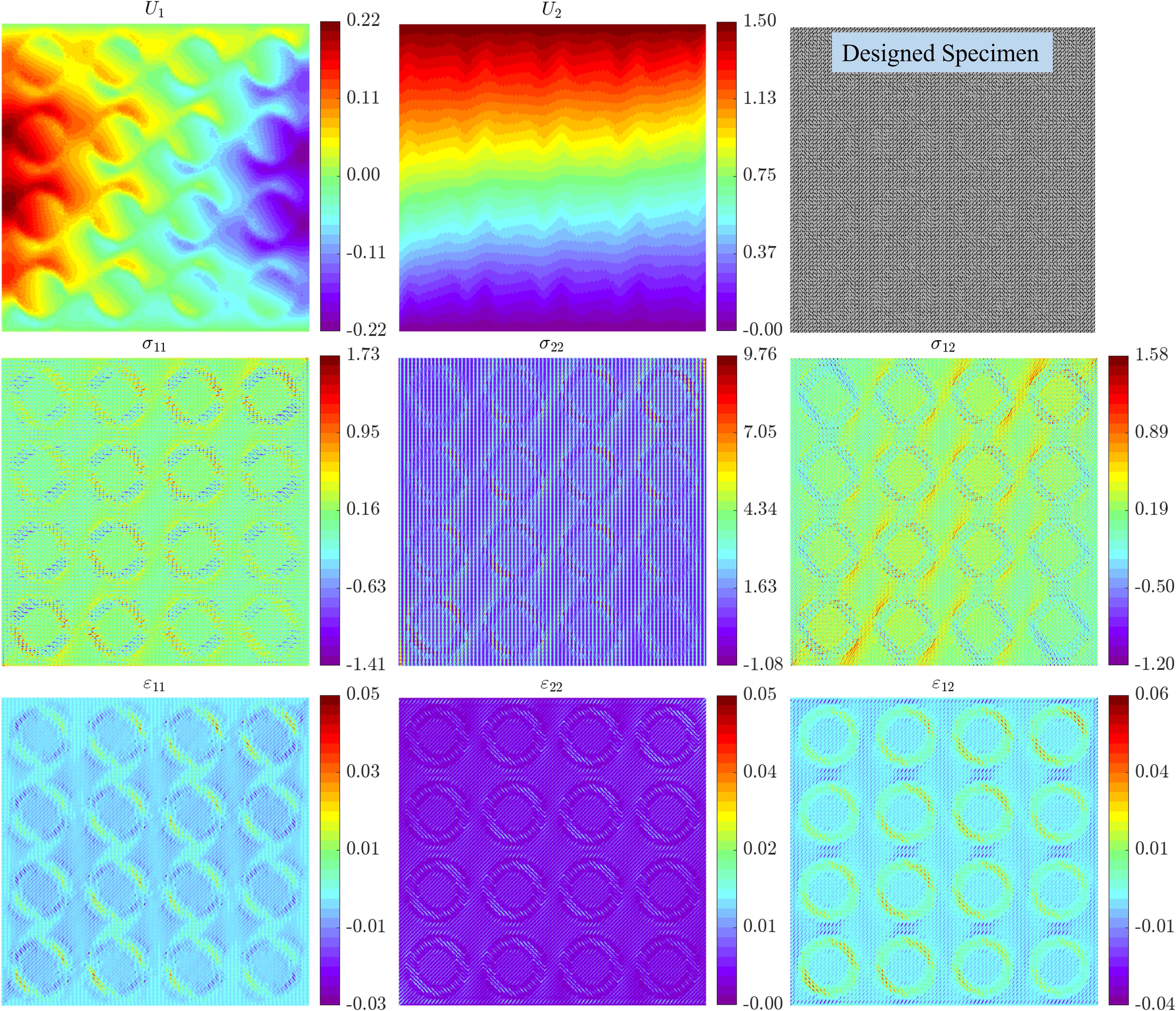
Further, we explore the mechanical behavior of a tessellation obtained by repeating the supercell 4 4 times. We define the supercell as the entire annular interpolated structure shown in Fig. 8 with 20 20 unit cells. In Fig. 9, we plot the displacement and strain contours from the FEA on this supercell tessellation subjected to tensile loading by prescribing a displacement of 1.5 mm 444Due to computational limitations, we limit our study to a 4 4 tessellation and reduce the unit cell size to 50 pixels from 100 pixels. For this 4 4 supercell tessellation, therefore, there are a total of unit cells resulting in a finite element mesh with elements.. We observe that the non-affine rotation-like deformations induced by geometric frustration are present in this supercell tessellation at all the annular regions. Additionally, there is an observed gradient in this non-affine behavior in the horizontal displacement component (). However, the magnitude of the horizontal displacement is reduced compared to the single supercell. There are non-local interactions from the neighboring annular regions. Similar behavior is observed in the case of supercell tessellation of example #2, as shown in Fig. S16. This suggests that the length scale as well as the separation between the annular regions play a significant role in affecting this rotation-like behavior, indicating the need to utilize micropolar elasticity in the context of such non-affine deformations in mechanical metamaterials (Lemkalli et al., 2023).
In the future, a detailed investigation into this scale dependence could be conducted using a multi-scale homogenization approach. Further, it is interesting to note that when this structure is subjected to simple shear loading no distinct non-affine deformation is observed, as the unit cells don’t differ in the shear-modulus like parameter . Therefore, investigations on the role of incompatibilities in other moduli may unveil new insights into graded structures experiencing geometric frustration under other complex loading conditions. Finally, exploring other choices of unit cells with contrasting moduli interpolated non-linearly could reveal unseen atypical mechanical behavior, which we leave for future work. In metallic materials with microstructure, defects such as grains and grain boundaries serve as strengthening mechanisms by creating incompatibilities that obstruct simple deformation paths. For example, twin boundaries that arise when a sufficiently high shear load is applied, act as an energy dissipation mechanism contributing to the plasticity of various metals. Therefore, the nonlinear interpolations introduced in this work could be utilized to design strengthening mechanisms in metamaterials, notably for energy dissipation and impact loading, extending beyond lattice materials as discussed further in Pham et al. (2019).
5 Conclusions
In this paper, we estimate the range of anisotropic stiffness tensors achieved by single-scale two-dimensional structured materials. We compare the property ranges reached by these single-scale architected materials with the extensive property space achieved by hierarchical laminates. In all property plots, we observed that rank-2 laminates significantly broaden the property range compared to rank-1 laminates We identify regions in the property space, particularly focusing on off-axis shear-normal coupling parameters, where hierarchical designs or the use of two anisotropic constituent phases are necessary to cover a wide property space. The bounds estimated alongside the unit cell database could serve as a design tool for the design of extremal metamaterials. By utilizing unit cells with extreme anisotropy that lie on the property gamut boundary, we design and fabricate functionally graded metamaterials exhibiting behaviors such as energy localization and localized rotations. These behaviors are atypical to the corresponding boundary conditions, arising from incompatibilities in the deformation modes of the unit cells. We then established the concept of supercells which were created by tessellating an entire annular graded structure. In supercell designs, we observed that the annular regions displayed non-local interactions leading to length-scale dependent behavior.
Although our study primarily focused on exploring 2D linear elastic properties, the proposed method has the potential to estimate similar bounds for three-dimensional structured materials with shear-shear coupling. The diverse range of geometries compiled in our database could also prove useful for studying nonlinear phenomena such as dispersive wave propagation, and viscoelastic behavior in two-phase composites. Furthermore, the exploration of other supercell tessellations incorporating different nonlinear interpolation schemes could potentially open up new avenues in the design of multi-scale metamaterials.
Acknowledgments
We would like to thank Prof. Kaushik Bhattacharya (Caltech), Prof. Graeme Milton (University of Utah), and Dr. Andrew Akerson (Caltech) for helpful discussions on the theoretical bounds of the elasticity tensors; C.D. and J.B. acknowledge the financial support from the US National Science Foundation (NSF) grant number 1835735, and MURI ARO W911NF-22-2-0109.
Appendix A Database of Elasticity Tensors
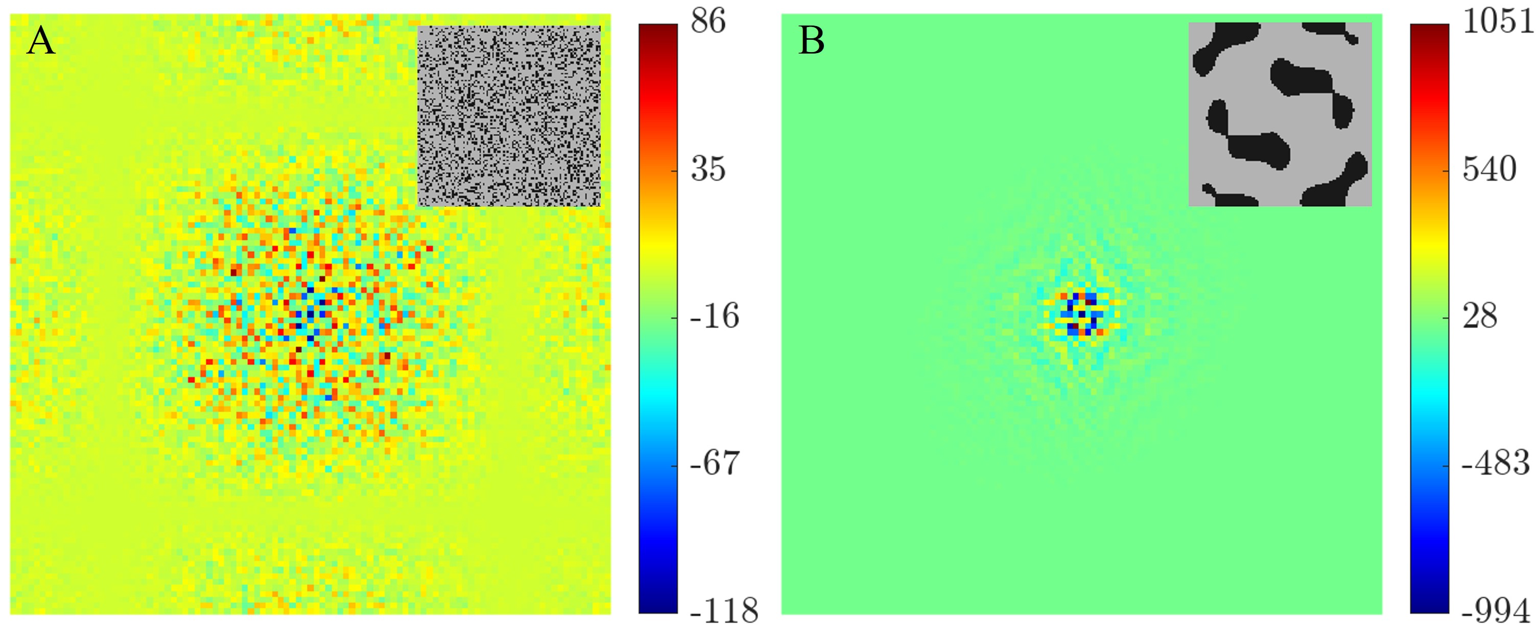
A.1 Fourier analysis of pixelated geometries
Here, we justify the selection of cosine functions for unit cell database generation. Two unit cells are considered for comparison: the first unit cell is randomly generated, lacking distinctive patterns, and appearing almost noisy; the second is obtained using the method in Section 2. After Gaussian filtering, the Fourier spectrum of both unit cells is shown in Fig. 10. To better illustrate the distribution of frequencies, the zero-frequency component, which represents the image’s mean value and has the highest magnitude, is removed from the plots. For the almost noisy unit cell, the spectrum shows peaks across a wide range of spatial frequencies. In contrast, the second unit cell’s spectrum is concentrated at lower spatial frequencies. This concentration justifies our choice of representation with very small spatial frequencies for generating the unit cells studied in this paper.
A.2 Non-square unit cell data generation
In a 2D periodic system, the unit cells can be rectangular, square, parallelogram-shaped, or irregularly hexagonal. Using the concepts of Bravais lattices and Brillouin zone, it is sufficient to consider an arbitrary parallelogram-shaped unit cell defined by the side lengths and the angle between the edges , to describe all possible unit cell shapes completely (Podestá et al., 2019). The values for parallelogram would give an equivalent regular hexagonal unit cell. Therefore, to generate non-square unit cell data, we considered several non-square oblique unit cells when the angle parameter is varied such that , while the ratio of side length is varied such that .
A.3 Theory of bounds on anisotropic elasticity tensors
For isotropic composites, Hashin and Shtrikman (1961, 1962) introduced a variational approach to determine the upper and lower bounds on the effective bulk and shear moduli ( and ) by decomposing the elastic energy into hydrostatic and deviatoric parts. However, the elastic energy cannot be decomposed to obtain variational bounds on the independent moduli in the anisotropic case. Recently Milton et al. (2017) and Milton and Camar-Eddine (2018) addressed this problem in terms of the stress and strain energy pairs and establishing bounds on the sum of the elastic and the complementary energies. Let the four energy functions , that characterize the set of possible elastic tensors be defined by
| (4a) | ||||
| (4b) | ||||
| (4c) | ||||
| (4d) | ||||
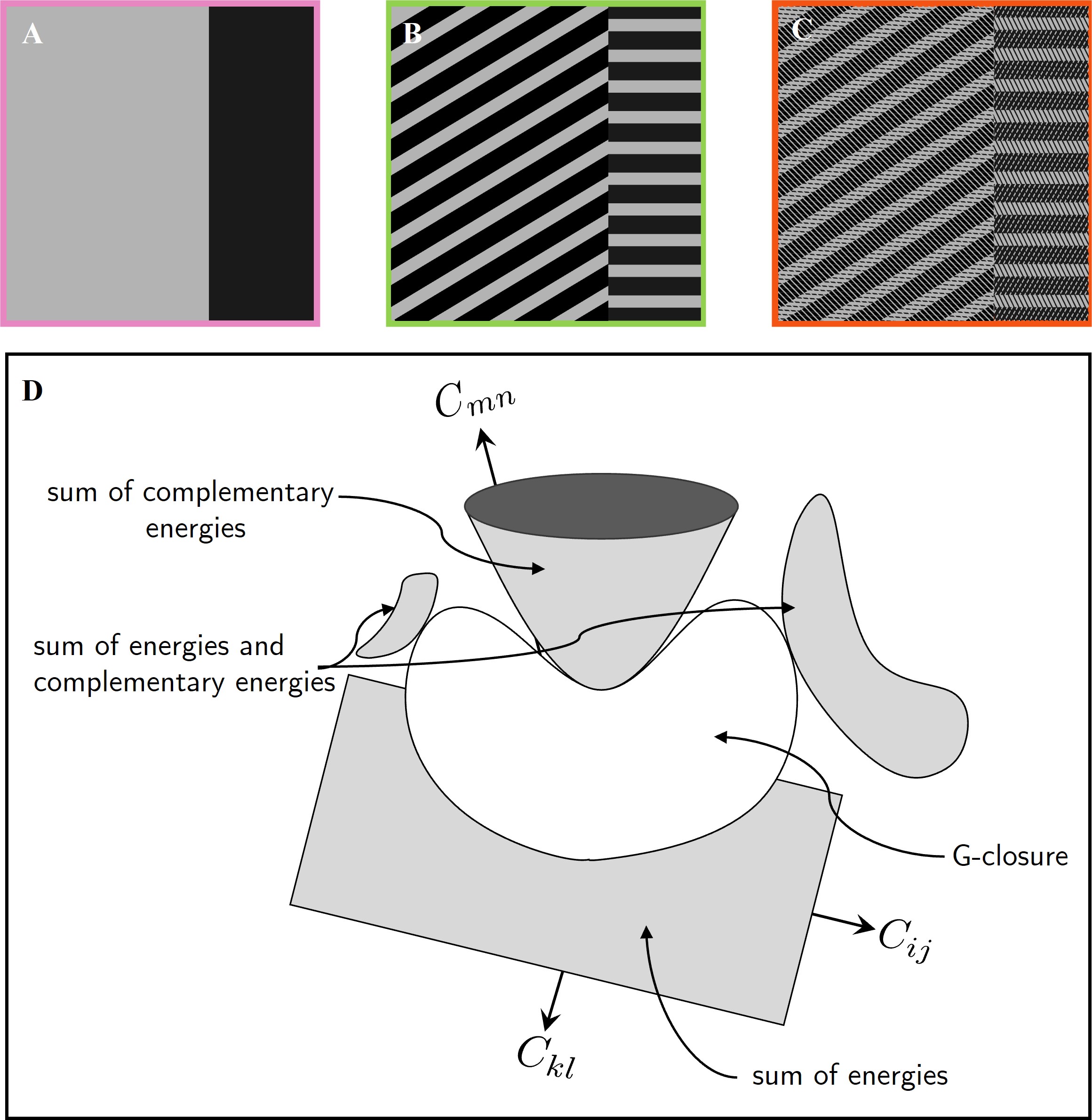
Each energy function , here represents the sum of three elastic energies, each obtained from an experiment where the composite, with effective tensor , is either subject to an applied stress or an applied strain . A total of three stresses and are applied simultaneously on the composite. The optimization of these energies to find for the applied stresses and strains is non-trivial. However, applying the key conclusions from (Willis, 1977; Avellaneda, 1987; Allaire and Kohn, 1993), Milton et al. (2017); Milton and Camar-Eddine (2018) discuss how sequentially layered laminates (or hierarchical laminates) minimize the sum of energies and complementary energies. In other words, G-closure can be seen as the G-closure of hierarchical laminates which is explained in Fig. 11. In two-dimensions, it is sufficient to consider laminates up to rank-3, if the constituent phases are isotropic. It is also worth noting that hierarchical laminates, with isotropic type effective elasticity tensor, simultaneously achieve Hashin-Shtrikman bulk and shear bounds (Francfort and Murat, 1986).
A.4 Construction of hierarchical laminates
Multiple-rank laminate materials are hierarchical materials created through an iterative lamination process at increasingly larger length scales. A rank-one laminate consists of two isotropic phases, which can be viewed as rank-zero laminates. A rank-() laminate is formed by layering a rank-() laminate with a laminate of rank-() or lower, as shown in Fig. 11. In two dimensions, it is sufficient to consider laminates up to rank-3 to estimate theoretical bounds, especially when the constituent materials are isotropic, as the 2D elasticity tensor has only three eigenvalues. Rank-1 laminates typically have one very high non-zero eigenvalue and two near-zero eigenvalues, while rank-2 laminates have two very high non-zero eigenvalues and one near-zero eigenvalue. To compute the effective properties of a higher rank- laminate, the constituent phases are replaced from isotropic to the relevant anisotropic phases of rank- laminates (See Figs. S4, S5 and S6). A rank-1 laminate is strictly defined by two parameters, the fill fraction of the stiff phase and the angle of orientation of the lamination. A rank-2 laminate is defined by four extra parameters the fill fraction of the stiff phase and the angle of orientation of each of the phases of the previous rank-1 laminate. Similarly, a rank-3 laminate is defined by eight extra parameters. Suppose, there are 11 different fill fractions and 18 different laminate orientations. This results in a total of elasticity tensors for rank-1 laminates. For rank-2 laminates, the total number of possible elasticity tensors is . For rank-3 laminates, the number increases to . First, the effective properties of all the rank-1 laminates are obtained by using two isotropic constituent phases for homogenization. To compute the effective properties of higher rank- laminates, the constituent phases are replaced from isotropic to the relevant anisotropic phases of lower rank(See Figs. S4, S5 and S6). To reduce the number of computations for the rank-3 laminates database, a subset of randomly chosen rank-2 elasticity tensors (about 1%) are used.
References
- Agnelli et al. (2021) Agnelli, F., Margerit, P., Celli, P., Daraio, C., Constantinescu, A., 2021. Systematic two-scale image analysis of extreme deformations in soft architectured sheets. International Journal of Mechanical Sciences 194, 106205. URL: https://www.sciencedirect.com/science/article/pii/S0020740320343101, doi:10.1016/j.ijmecsci.2020.106205.
- Agnelli et al. (2022) Agnelli, F., Nika, G., Constantinescu, A., 2022. Design of thin micro-architectured panels with extension–bending coupling effects using topology optimization. Computer Methods in Applied Mechanics and Engineering 391, 114496. URL: https://www.sciencedirect.com/science/article/pii/S0045782521007040, doi:10.1016/j.cma.2021.114496.
- Allaire and Kohn (1993) Allaire, G., Kohn, R.V., 1993. Optimal bounds on the effective behavior of a mixture of two well-ordered elastic materials. Quarterly of Applied Mathematics 51, 643–674. URL: https://www.ams.org/qam/1993-51-04/S0033-569X-1993-1247433-7/, doi:10.1090/qam/1247433.
- Andreassen and Andreasen (2014) Andreassen, E., Andreasen, C.S., 2014. How to determine composite material properties using numerical homogenization. Computational Materials Science 83, 488–495. URL: https://www.sciencedirect.com/science/article/pii/S0927025613005302, doi:10.1016/j.commatsci.2013.09.006.
- Antimonov et al. (2016) Antimonov, M.A., Cherkaev, A., Freidin, A.B., 2016. Phase transformations surfaces and exact energy lower bounds. International Journal of Engineering Science 98, 153–182. URL: https://linkinghub.elsevier.com/retrieve/pii/S0020722515001408, doi:10.1016/j.ijengsci.2015.10.004.
- Avellaneda (1987) Avellaneda, M., 1987. Optimal Bounds and Microgeometries for Elastic Two-Phase Composites. SIAM Journal on Applied Mathematics 47, 1216–1228. URL: https://epubs.siam.org/doi/10.1137/0147082, doi:10.1137/0147082. publisher: Society for Industrial and Applied Mathematics.
- Bastek and Kochmann (2023) Bastek, J.H., Kochmann, D.M., 2023. Inverse design of nonlinear mechanical metamaterials via video denoising diffusion models. Nature Machine Intelligence 5, 1466–1475. URL: https://www.nature.com/articles/s42256-023-00762-x, doi:10.1038/s42256-023-00762-x. number: 12 Publisher: Nature Publishing Group.
- Bastek et al. (2022) Bastek, J.H., Kumar, S., Telgen, B., Glaesener, R.N., Kochmann, D.M., 2022. Inverting the structure–property map of truss metamaterials by deep learning. Proceedings of the National Academy of Sciences 119, e2111505119. URL: https://www.pnas.org/doi/abs/10.1073/pnas.2111505119, doi:10.1073/pnas.2111505119. publisher: Proceedings of the National Academy of Sciences.
- Boddapati et al. (2023) Boddapati, J., Flaschel, M., Kumar, S., De Lorenzis, L., Daraio, C., 2023. Single-test evaluation of directional elastic properties of anisotropic structured materials. Journal of the Mechanics and Physics of Solids 181, 105471. URL: https://www.sciencedirect.com/science/article/pii/S0022509623002752, doi:10.1016/j.jmps.2023.105471.
- Bückmann et al. (2014) Bückmann, T., Thiel, M., Kadic, M., Schittny, R., Wegener, M., 2014. An elasto-mechanical unfeelability cloak made of pentamode metamaterials. Nature Communications 5, 4130. URL: https://www.nature.com/articles/ncomms5130, doi:10.1038/ncomms5130. number: 1 Publisher: Nature Publishing Group.
- Cahn (1965) Cahn, J.W., 1965. Phase Separation by Spinodal Decomposition in Isotropic Systems. The Journal of Chemical Physics 42, 93–99. URL: https://pubs.aip.org/jcp/article/42/1/93/81515/Phase-Separation-by-Spinodal-Decomposition-in, doi:10.1063/1.1695731.
- Chen et al. (2023) Chen, D., Gao, K., Yang, J., Zhang, L., 2023. Functionally graded porous structures: Analyses, performances, and applications – A Review. Thin-Walled Structures 191, 111046. URL: https://www.sciencedirect.com/science/article/pii/S0263823123005244, doi:10.1016/j.tws.2023.111046.
- Chen et al. (2018) Chen, D., Skouras, M., Zhu, B., Matusik, W., 2018. Computational discovery of extremal microstructure families. Science Advances 4, eaao7005. URL: https://www.science.org/doi/10.1126/sciadv.aao7005, doi:10.1126/sciadv.aao7005.
- Chenchiah and Bhattacharya (2008) Chenchiah, I.V., Bhattacharya, K., 2008. The Relaxation of Two-well Energies with Possibly Unequal Moduli. Archive for Rational Mechanics and Analysis 187, 409–479. URL: https://doi.org/10.1007/s00205-007-0075-3, doi:10.1007/s00205-007-0075-3.
- Cherkaev and Gibiansky (1993) Cherkaev, A.V., Gibiansky, L.V., 1993. Coupled estimates for the bulk and shear moduli of a two-dimensional isotropic elastic composite. Journal of the Mechanics and Physics of Solids 41, 937–980. URL: https://www.sciencedirect.com/science/article/pii/0022509693900062, doi:10.1016/0022-5096(93)90006-2.
- Diaz and Bénard (2003) Diaz, A.R., Bénard, A., 2003. Designing materials with prescribed elastic properties using polygonal cells. International Journal for Numerical Methods in Engineering 57, 301–314. URL: https://onlinelibrary.wiley.com/doi/abs/10.1002/nme.677, doi:10.1002/nme.677. _eprint: https://onlinelibrary.wiley.com/doi/pdf/10.1002/nme.677.
- Ellenbroek et al. (2009) Ellenbroek, W.G., Zeravcic, Z., Saarloos, W.v., Hecke, M.v., 2009. Non-affine response: Jammed packings vs. spring networks. Europhysics Letters 87, 34004. URL: https://dx.doi.org/10.1209/0295-5075/87/34004, doi:10.1209/0295-5075/87/34004.
- Feyrer (2007) Feyrer, K., 2007. Wire Ropes. Springer, Berlin, Heidelberg. URL: http://link.springer.com/10.1007/978-3-540-33831-4, doi:10.1007/978-3-540-33831-4.
- Fleck et al. (2010) Fleck, N.A., Deshpande, V.S., Ashby, M.F., 2010. Micro-architectured materials: past, present and future. Proceedings of the Royal Society A: Mathematical, Physical and Engineering Sciences 466, 2495–2516. URL: https://royalsocietypublishing.org/doi/full/10.1098/rspa.2010.0215, doi:10.1098/rspa.2010.0215. publisher: Royal Society.
- Forte and Vianello (2014) Forte, S., Vianello, M., 2014. A unified approach to invariants of plane elasticity tensors. Meccanica 49, 2001–2012. URL: http://link.springer.com/10.1007/s11012-014-9916-y, doi:10.1007/s11012-014-9916-y.
- Francfort and Milton (1994) Francfort, G.A., Milton, G.W., 1994. Sets of conductivity and elasticity tensors stable under lamination. Communications on Pure and Applied Mathematics 47, 257–279. URL: https://onlinelibrary.wiley.com/doi/abs/10.1002/cpa.3160470302, doi:10.1002/cpa.3160470302. _eprint: https://onlinelibrary.wiley.com/doi/pdf/10.1002/cpa.3160470302.
- Francfort and Murat (1986) Francfort, G.A., Murat, F., 1986. Homogenization and optimal bounds in linear elasticity. Archive for Rational Mechanics and Analysis 94, 307–334. URL: https://doi.org/10.1007/BF00280908, doi:10.1007/BF00280908.
- Freidin (2007) Freidin, A., 2007. On new phase inclusions in elastic solids. ZAMM 87, 102–116. URL: https://onlinelibrary.wiley.com/doi/10.1002/zamm.200610305, doi:10.1002/zamm.200610305.
- Freidin and Sharipova (2019) Freidin, A.B., Sharipova, L.L., 2019. Two-phase equilibrium microstructures against optimal composite microstructures. Archive of Applied Mechanics 89, 561–580. URL: http://link.springer.com/10.1007/s00419-019-01510-7, doi:10.1007/s00419-019-01510-7.
- Garner et al. (2019) Garner, E., Kolken, H.M.A., Wang, C.C.L., Zadpoor, A.A., Wu, J., 2019. Compatibility in microstructural optimization for additive manufacturing. Additive Manufacturing 26, 65–75. URL: https://www.sciencedirect.com/science/article/pii/S2214860418306808, doi:10.1016/j.addma.2018.12.007.
- Gibson and Ashby (1997) Gibson, L.J., Ashby, M.F., 1997. Cellular Solids: Structure and Properties. Cambridge Solid State Science Series. 2 ed., Cambridge University Press, Cambridge. URL: https://www.cambridge.org/core/books/cellular-solids/BC25789552BAA8E3CAD5E1D105612AB5, doi:10.1017/CBO9781139878326.
- Gupta and Meena (2023) Gupta, K., Meena, K., 2023. Artificial bone scaffolds and bone joints by additive manufacturing: A review. Bioprinting 31, e00268. URL: https://www.sciencedirect.com/science/article/pii/S2405886623000118, doi:10.1016/j.bprint.2023.e00268.
- Hashin and Shtrikman (1961) Hashin, Z., Shtrikman, S., 1961. Note on a variational approach to the theory of composite elastic materials. Journal of the Franklin Institute 271, 336–341. URL: https://linkinghub.elsevier.com/retrieve/pii/0016003261900321, doi:10.1016/0016-0032(61)90032-1.
- Hashin and Shtrikman (1962) Hashin, Z., Shtrikman, S., 1962. On some variational principles in anisotropic and nonhomogeneous elasticity. Journal of the Mechanics and Physics of Solids 10, 335–342. URL: https://www.sciencedirect.com/science/article/pii/0022509662900042, doi:10.1016/0022-5096(62)90004-2.
- Hild and Roux (2012) Hild, F., Roux, S., 2012. Comparison of Local and Global Approaches to Digital Image Correlation. Experimental Mechanics 52, 1503–1519. URL: https://doi.org/10.1007/s11340-012-9603-7, doi:10.1007/s11340-012-9603-7.
- Hu et al. (2023) Hu, Z., Wei, Z., Wang, K., Chen, Y., Zhu, R., Huang, G., Hu, G., 2023. Engineering zero modes in transformable mechanical metamaterials. Nature Communications 14, 1266. URL: https://www.nature.com/articles/s41467-023-36975-2, doi:10.1038/s41467-023-36975-2. number: 1 Publisher: Nature Publishing Group.
- Karathanasopoulos et al. (2020) Karathanasopoulos, N., Dos Reis, F., Diamantopoulou, M., Ganghoffer, J.F., 2020. Mechanics of beams made from chiral metamaterials: Tuning deflections through normal-shear strain couplings. Materials & Design 189, 108520. URL: https://www.sciencedirect.com/science/article/pii/S0264127520300538, doi:10.1016/j.matdes.2020.108520.
- Kumar et al. (2020) Kumar, S., Tan, S., Zheng, L., Kochmann, D.M., 2020. Inverse-designed spinodoid metamaterials. npj Computational Materials 6, 73. URL: http://www.nature.com/articles/s41524-020-0341-6, doi:10.1038/s41524-020-0341-6.
- Lee et al. (2024a) Lee, D., Chen, W.W., Wang, L., Chan, Y.C., Chen, W., 2024a. Data-Driven Design for Metamaterials and Multiscale Systems: A Review. Advanced Materials 36, 2305254. URL: https://onlinelibrary.wiley.com/doi/abs/10.1002/adma.202305254, doi:10.1002/adma.202305254. _eprint: https://onlinelibrary.wiley.com/doi/pdf/10.1002/adma.202305254.
- Lee et al. (2022) Lee, G., Lee, D., Park, J., Jang, Y., Kim, M., Rho, J., 2022. Piezoelectric energy harvesting using mechanical metamaterials and phononic crystals. Communications Physics 5, 1–16. URL: https://www.nature.com/articles/s42005-022-00869-4, doi:10.1038/s42005-022-00869-4. publisher: Nature Publishing Group.
- Lee et al. (2023) Lee, G., Lee, S.J., Rho, J., Kim, M., 2023. Acoustic and mechanical metamaterials for energy harvesting and self-powered sensing applications. Materials Today Energy 37, 101387. URL: https://www.sciencedirect.com/science/article/pii/S2468606923001430, doi:10.1016/j.mtener.2023.101387.
- Lee and Kim (2023) Lee, J., Kim, Y.Y., 2023. Elastic metamaterials for guided waves: from fundamentals to applications. Smart Materials and Structures 32, 123001. URL: https://dx.doi.org/10.1088/1361-665X/ad0393, doi:10.1088/1361-665X/ad0393. publisher: IOP Publishing.
- Lee et al. (2024b) Lee, W., Lee, J., Park, C.I., Kim, Y.Y., 2024b. Polarization-independent full mode-converting elastic metasurfaces. International Journal of Mechanical Sciences 266, 108975. URL: https://www.sciencedirect.com/science/article/pii/S0020740324000183, doi:10.1016/j.ijmecsci.2024.108975.
- Lemkalli et al. (2023) Lemkalli, B., Kadic, M., El Badri, Y., Guenneau, S., Bouzid, A., Achaoui, Y., 2023. Mapping of elastic properties of twisting metamaterials onto micropolar continuum using static calculations. International Journal of Mechanical Sciences 254, 108411. URL: https://www.sciencedirect.com/science/article/pii/S0020740323003132, doi:10.1016/j.ijmecsci.2023.108411.
- Li et al. (2018) Li, H., Luo, Z., Gao, L., Walker, P., 2018. Topology optimization for functionally graded cellular composites with metamaterials by level sets. Computer Methods in Applied Mechanics and Engineering 328, 340–364. URL: https://www.sciencedirect.com/science/article/pii/S0045782516310106, doi:10.1016/j.cma.2017.09.008.
- Li et al. (2024) Li, X., Wang, P., Zhao, M., Su, X., Tan, Y.H., Ding, J., 2024. Customizable anisotropic microlattices for additive manufacturing: Machine learning accelerated design, mechanical properties and structural-property relationships. Additive Manufacturing 89, 104248. URL: https://www.sciencedirect.com/science/article/pii/S221486042400294X, doi:10.1016/j.addma.2024.104248.
- Liu and Hu (2016) Liu, X., Hu, G., 2016. Elastic Metamaterials Making Use of Chirality: A Review. Strojniški vestnik - Journal of Mechanical Engineering 62, 403–418. URL: http://www.sv-jme.eu/article/elastic-metamaterials-making-use-of-chirality-a-review/, doi:10.5545/sv-jme.2016.3799.
- Luan et al. (2023) Luan, S., Chen, E., John, J., Gaitanaros, S., 2023. A data-driven framework for structure-property correlation in ordered and disordered cellular metamaterials. Science Advances 9, eadi1453. URL: https://www.science.org/doi/10.1126/sciadv.adi1453, doi:10.1126/sciadv.adi1453. publisher: American Association for the Advancement of Science.
- Lumpe and Stankovic (2021) Lumpe, T.S., Stankovic, T., 2021. Exploring the property space of periodic cellular structures based on crystal networks. Proceedings of the National Academy of Sciences 118, e2003504118. URL: https://pnas.org/doi/full/10.1073/pnas.2003504118, doi:10.1073/pnas.2003504118.
- Mao et al. (2020) Mao, Y., He, Q., Zhao, X., 2020. Designing complex architectured materials with generative adversarial networks. Science Advances 6, eaaz4169. URL: https://www.science.org/doi/10.1126/sciadv.aaz4169, doi:10.1126/sciadv.aaz4169.
- Maurizi et al. (2022) Maurizi, M., Gao, C., Berto, F., 2022. Inverse design of truss lattice materials with superior buckling resistance. npj Computational Materials 8, 1–12. URL: https://www.nature.com/articles/s41524-022-00938-w, doi:10.1038/s41524-022-00938-w. number: 1 Publisher: Nature Publishing Group.
- Milton et al. (2017) Milton, G., Briane, M., Harutyunyan, D., 2017. On the possible effective elasticity tensors of 2-dimensional and 3-dimensional printed materials. Mathematics and Mechanics of Complex Systems 5, 41–94. URL: http://msp.org/memocs/2017/5-1/p03.xhtml, doi:10.2140/memocs.2017.5.41.
- Milton (2021) Milton, G.W., 2021. Some open problems in the theory of composites. Philosophical Transactions of the Royal Society A: Mathematical, Physical and Engineering Sciences 379, 20200115. URL: https://royalsocietypublishing.org/doi/10.1098/rsta.2020.0115, doi:10.1098/rsta.2020.0115. publisher: Royal Society.
- Milton (2022) Milton, G.W., 2022. Chapter 30: Properties of the G-closure and extremal families of composites, in: The Theory of Composites. Society for Industrial and Applied Mathematics. Classics in Applied Mathematics, pp. 643–669. URL: https://epubs.siam.org/doi/10.1137/1.9781611977486.ch30, doi:10.1137/1.9781611977486.ch30.
- Milton and Camar-Eddine (2018) Milton, G.W., Camar-Eddine, M., 2018. Near optimal pentamodes as a tool for guiding stress while minimizing compliance in 3d-printed materials: A complete solution to the weak G-closure problem for 3d-printed materials. Journal of the Mechanics and Physics of Solids 114, 194–208. URL: https://www.sciencedirect.com/science/article/pii/S0022509617310967, doi:10.1016/j.jmps.2018.02.003.
- Milton and Cherkaev (1995) Milton, G.W., Cherkaev, A.V., 1995. Which Elasticity Tensors are Realizable? Journal of Engineering Materials and Technology 117, 483–493. URL: https://doi.org/10.1115/1.2804743, doi:10.1115/1.2804743.
- Milton and Kohn (1988) Milton, G.W., Kohn, R.V., 1988. Variational bounds on the effective moduli of anisotropic composites. Journal of the Mechanics and Physics of Solids 36, 597–629. URL: https://www.sciencedirect.com/science/article/pii/0022509688900014, doi:10.1016/0022-5096(88)90001-4.
- Nepal et al. (2023) Nepal, D., Kang, S., Adstedt, K.M., Kanhaiya, K., Bockstaller, M.R., Brinson, L.C., Buehler, M.J., Coveney, P.V., Dayal, K., El-Awady, J.A., Henderson, L.C., Kaplan, D.L., Keten, S., Kotov, N.A., Schatz, G.C., Vignolini, S., Vollrath, F., Wang, Y., Yakobson, B.I., Tsukruk, V.V., Heinz, H., 2023. Hierarchically structured bioinspired nanocomposites. Nature Materials 22, 18–35. URL: https://www.nature.com/articles/s41563-022-01384-1, doi:10.1038/s41563-022-01384-1. publisher: Nature Publishing Group.
- Oh et al. (2023) Oh, S., Song, T.E., Mahato, M., Kim, J.S., Yoo, H., Lee, M.J., Khan, M., Yeo, W.H., Oh, I.K., 2023. Easy-To-Wear Auxetic SMA Knot-Architecture for Spatiotemporal and Multimodal Haptic Feedbacks. Advanced Materials 35, 2304442. URL: https://onlinelibrary.wiley.com/doi/abs/10.1002/adma.202304442, doi:10.1002/adma.202304442. _eprint: https://onlinelibrary.wiley.com/doi/pdf/10.1002/adma.202304442.
- Ostanin et al. (2018) Ostanin, I., Ovchinnikov, G., Tozoni, D.C., Zorin, D., 2018. A parametric class of composites with a large achievable range of effective elastic properties. Journal of the Mechanics and Physics of Solids 118, 204–217. URL: https://www.sciencedirect.com/science/article/pii/S0022509617311183, doi:10.1016/j.jmps.2018.05.018.
- Panesar et al. (2018) Panesar, A., Abdi, M., Hickman, D., Ashcroft, I., 2018. Strategies for functionally graded lattice structures derived using topology optimisation for Additive Manufacturing. Additive Manufacturing 19, 81–94. URL: https://www.sciencedirect.com/science/article/pii/S221486041730115X, doi:10.1016/j.addma.2017.11.008.
- Panetta et al. (2015) Panetta, J., Zhou, Q., Malomo, L., Pietroni, N., Cignoni, P., Zorin, D., 2015. Elastic textures for additive fabrication. ACM Transactions on Graphics 34, 1–12. URL: https://dl.acm.org/doi/10.1145/2766937, doi:10.1145/2766937.
- Pham et al. (2019) Pham, M.S., Liu, C., Todd, I., Lertthanasarn, J., 2019. Damage-tolerant architected materials inspired by crystal microstructure. Nature 565, 305–311. URL: https://www.nature.com/articles/s41586-018-0850-3, doi:10.1038/s41586-018-0850-3. publisher: Nature Publishing Group.
- Podestá et al. (2019) Podestá, J., Méndez, C., Toro, S., Huespe, A., 2019. Symmetry considerations for topology design in the elastic inverse homogenization problem. Journal of the Mechanics and Physics of Solids 128, 54–78. URL: https://linkinghub.elsevier.com/retrieve/pii/S0022509618305210, doi:10.1016/j.jmps.2019.03.018.
- Rubinstein and Panyukov (1997) Rubinstein, M., Panyukov, S., 1997. Nonaffine Deformation and Elasticity of Polymer Networks. Macromolecules 30, 8036–8044. URL: https://doi.org/10.1021/ma970364k, doi:10.1021/ma970364k. publisher: American Chemical Society.
- Sanders et al. (2021) Sanders, E.D., Pereira, A., Paulino, G.H., 2021. Optimal and continuous multilattice embedding. Science Advances 7, eabf4838. URL: https://www.science.org/doi/10.1126/sciadv.abf4838, doi:10.1126/sciadv.abf4838. publisher: American Association for the Advancement of Science.
- Saxena et al. (2016) Saxena, K.K., Das, R., Calius, E.P., 2016. Three Decades of Auxetics Research - Materials with Negative Poisson’s Ratio: A Review. Advanced Engineering Materials 18, 1847–1870. URL: https://onlinelibrary.wiley.com/doi/abs/10.1002/adem.201600053, doi:10.1002/adem.201600053. _eprint: https://onlinelibrary.wiley.com/doi/pdf/10.1002/adem.201600053.
- Schreier et al. (2009) Schreier, H., Orteu, J.J., Sutton, M.A., 2009. Image Correlation for Shape, Motion and Deformation Measurements: Basic Concepts,Theory and Applications. Springer US, Boston, MA. URL: https://link.springer.com/10.1007/978-0-387-78747-3, doi:10.1007/978-0-387-78747-3.
- Schumacher et al. (2015) Schumacher, C., Bickel, B., Rys, J., Marschner, S., Daraio, C., Gross, M., 2015. Microstructures to control elasticity in 3D printing. ACM Transactions on Graphics 34, 1–13. URL: https://dl.acm.org/doi/10.1145/2766926, doi:10.1145/2766926.
- Sigmund (2000) Sigmund, O., 2000. A new class of extremal composites. Journal of the Mechanics and Physics of Solids 48, 397–428. URL: https://www.sciencedirect.com/science/article/pii/S0022509699000344, doi:10.1016/S0022-5096(99)00034-4.
- Sigmund (2009) Sigmund, O., 2009. Systematic Design of Metamaterials by Topology Optimization, in: Pyrz, R., Rauhe, J.C. (Eds.), IUTAM Symposium on Modelling Nanomaterials and Nanosystems, Springer Netherlands, Dordrecht. pp. 151–159. doi:10.1007/978-1-4020-9557-3_16.
- Soyarslan et al. (2018) Soyarslan, C., Bargmann, S., Pradas, M., Weissmüller, J., 2018. 3D stochastic bicontinuous microstructures: Generation, topology and elasticity. Acta Materialia 149, 326–340. URL: https://www.sciencedirect.com/science/article/pii/S1359645418300363, doi:10.1016/j.actamat.2018.01.005.
- Surjadi et al. (2019) Surjadi, J.U., Gao, L., Du, H., Li, X., Xiong, X., Fang, N.X., Lu, Y., 2019. Mechanical Metamaterials and Their Engineering Applications. Advanced Engineering Materials 21, 1800864. URL: https://onlinelibrary.wiley.com/doi/abs/10.1002/adem.201800864, doi:10.1002/adem.201800864. _eprint: https://onlinelibrary.wiley.com/doi/pdf/10.1002/adem.201800864.
- Tavakoli and Costi (2018) Tavakoli, J., Costi, J.J., 2018. Ultrastructural organization of elastic fibres in the partition boundaries of the annulus fibrosus within the intervertebral disc. Acta Biomaterialia 68, 67–77. URL: https://www.sciencedirect.com/science/article/pii/S1742706117307833, doi:10.1016/j.actbio.2017.12.017.
- Tian et al. (2024) Tian, L., Sun, B., Yan, X., Sharf, A., Tu, C., Lu, L., 2024. Continuous transitions of triply periodic minimal surfaces. Additive Manufacturing 84, 104105. URL: https://www.sciencedirect.com/science/article/pii/S2214860424001519, doi:10.1016/j.addma.2024.104105.
- Tomita et al. (2023) Tomita, S., Shimanuki, K., Oyama, S., Nishigaki, H., Nakagawa, T., Tsutsui, M., Emura, Y., Chino, M., Tanaka, H., Itou, Y., Umemoto, K., 2023. Transition of deformation modes from bending to auxetic compression in origami-based metamaterials for head protection from impact. Scientific Reports 13, 12221. URL: https://www.nature.com/articles/s41598-023-39200-8, doi:10.1038/s41598-023-39200-8. publisher: Nature Publishing Group.
- Volandri et al. (2011) Volandri, G., Di Puccio, F., Forte, P., Carmignani, C., 2011. Biomechanics of the tympanic membrane. Journal of Biomechanics 44, 1219–1236. URL: https://www.sciencedirect.com/science/article/pii/S0021929011000224, doi:10.1016/j.jbiomech.2010.12.023.
- Wang et al. (2022) Wang, L., Boddapati, J., Liu, K., Zhu, P., Daraio, C., Chen, W., 2022. Mechanical cloak via data-driven aperiodic metamaterial design. Proceedings of the National Academy of Sciences 119, e2122185119. URL: https://pnas.org/doi/full/10.1073/pnas.2122185119, doi:10.1073/pnas.2122185119.
- Wang et al. (2020) Wang, L., Chan, Y.C., Ahmed, F., Liu, Z., Zhu, P., Chen, W., 2020. Deep generative modeling for mechanistic-based learning and design of metamaterial systems. Computer Methods in Applied Mechanics and Engineering 372, 113377. URL: https://www.sciencedirect.com/science/article/pii/S0045782520305624, doi:10.1016/j.cma.2020.113377.
- Willis (1977) Willis, J.R., 1977. Bounds and self-consistent estimates for the overall properties of anisotropic composites. Journal of the Mechanics and Physics of Solids 25, 185–202. URL: https://www.sciencedirect.com/science/article/pii/0022509677900229, doi:10.1016/0022-5096(77)90022-9.
- Wu et al. (2023) Wu, C., Luo, J., Zhong, J., Xu, Y., Wan, B., Huang, W., Fang, J., Steven, G.P., Sun, G., Li, Q., 2023. Topology optimisation for design and additive manufacturing of functionally graded lattice structures using derivative-aware machine learning algorithms. Additive Manufacturing 78, 103833. URL: https://www.sciencedirect.com/science/article/pii/S2214860423004463, doi:10.1016/j.addma.2023.103833.
- Wu et al. (2018) Wu, W., Song, X., Liang, J., Xia, R., Qian, G., Fang, D., 2018. Mechanical properties of anti-tetrachiral auxetic stents. Composite Structures 185, 381–392. URL: https://www.sciencedirect.com/science/article/pii/S0263822317324078, doi:10.1016/j.compstruct.2017.11.048.
- Yang et al. (2019) Yang, C., Kim, Y., Ryu, S., Gu, G.X., 2019. Using convolutional neural networks to predict composite properties beyond the elastic limit. MRS Communications 9, 609–617. URL: https://www.cambridge.org/core/journals/mrs-communications/article/using-convolutional-neural-networks-to-predict-composite-properties-beyond-the-elastic-limit/D58F4D59C1644EEB704B07D04F0CE220, doi:10.1557/mrc.2019.49. publisher: Cambridge University Press.
- Yu et al. (2017) Yu, S., Zhang, Y., Wang, C., Lee, W.k., Dong, B., Odom, T.W., Sun, C., Chen, W., 2017. Characterization and Design of Functional Quasi-Random Nanostructured Materials Using Spectral Density Function. Journal of Mechanical Design 139, 071401. URL: https://asmedigitalcollection.asme.org/mechanicaldesign/article/doi/10.1115/1.4036582/383763/Characterization-and-Design-of-Functional, doi:10.1115/1.4036582.
- Zhang and Lu (2002) Zhang, D., Lu, G., 2002. Shape-based image retrieval using generic Fourier descriptor. Signal Processing: Image Communication 17, 825–848. URL: https://www.sciencedirect.com/science/article/pii/S092359650200084X, doi:10.1016/S0923-5965(02)00084-X.
- Zhang et al. (2023) Zhang, Z., Brandt, C., Jouve, J., Wang, Y., Chen, T., Pauly, M., Panetta, J., 2023. Computational Design of Flexible Planar Microstructures. ACM Transactions on Graphics 42, 1–16. URL: https://dl.acm.org/doi/10.1145/3618396, doi:10.1145/3618396.
- Zheng et al. (2023a) Zheng, L., Karapiperis, K., Kumar, S., Kochmann, D.M., 2023a. Unifying the design space and optimizing linear and nonlinear truss metamaterials by generative modeling. Nature Communications 14, 7563. URL: https://www.nature.com/articles/s41467-023-42068-x, doi:10.1038/s41467-023-42068-x. number: 1 Publisher: Nature Publishing Group.
- Zheng et al. (2023b) Zheng, X., Zhang, X., Chen, T.T., Watanabe, I., 2023b. Deep Learning in Mechanical Metamaterials: From Prediction and Generation to Inverse Design. Advanced Materials 35, 2302530. URL: https://onlinelibrary.wiley.com/doi/abs/10.1002/adma.202302530, doi:10.1002/adma.202302530. _eprint: https://onlinelibrary.wiley.com/doi/pdf/10.1002/adma.202302530.
Supplementary Information
Appendix S-I Elasticity tensor invariants
Using harmonic decomposition (Forte and Vianello, 2014), the strain energy density () can be decomposed as,
| (S1a) | ||||
| (S1b) | ||||
where , , , are the spherical and deviatoric part of the stress and strain tensors respectively. Here Einstein’s notation of summation over repeated indices is used. , are defined as
| (S2a) | ||||
| (S2b) | ||||
where , , are the parameters obtained from harmonic decomposition of the elasticity tensor as
| (S3) |
where , , are all linear combinations of the elasticity tensor parameters.
is defined as
| (S4) |
is defined as
| (S5) |
is defined as
| (S6) |
is defined as
| (S7) | ||||
| (S8) |
Based on this decomposition, four invariants, that do not depend on the choice of the coordinate system of the material, are defined as follows.
is a measure of the sphericity of the material and is defined as
| (S9) |
is a measure of the isotropic part of the deviatoricity of the material and is defined as
| (S10) |
is the square of a norm that measures the amount of coupling energy in the material and is defined as
| (S11) |
measures the squared norm of the anisotropic part of the deviatoricity of the material and is defined as
| (S12) |
In the case of isotropic material, the invariants would be zero. A few insights on the trends in the property plots, as discussed in Section 3.2 are derived from the invariants.
Appendix S-II Experimental data acquisition
Fabrication: We fabricate the specimens using a commercial multi-material polyjet technology-based 3D printer, the Stratasys Objet500 Connex. The specimens measure 75 × 75 × 5 mm, not including the portion inserted into the grips. For the stiff phase, we use Stratasys’ proprietary material DM8530, and for the soft phase, TangoBlack. The material properties are experimentally determined following the ASTM D638-14 standard test method: DM8530 has a Young’s modulus (E) of 1000 90 MPa and a Poisson’s ratio () of 0.35, while TangoBlack has a Young’s modulus (E) of 0.7 MPa and a Poisson’s ratio () of 0.49.
Tension testing: We subject the additively manufactured specimens to displacement-controlled tension tests using a universal testing machine, Instron E3000. We apply a vertical displacement of 1.5 mm at the top boundary at a rate of 0.5 mm/min resulting in a global axial strain of and a global strain rate of s-1. Custom-designed grips are fabricated out of aluminum and are serrated to hold the specimens firmly and prevent any lateral slipping. We use the same strain rate while measuring the constitutive material properties of the individual phases. We repeated the experiments on three different specimens for the same design. All the specimens showed little variation in the observed global behavior.
Digital image correlation: We use DIC, an image-based optical technique, to measure the full-field displacements (Schreier et al., 2009; Hild and Roux, 2012). We capture images at a frequency of 1 Hz using a Nikon D750 camera equipped with a Nikon AF-S NIKKOR 24-120mm f/4G ED VR zoom lens. We use manual mode at an exposure rate of 1/640 sec, an ISO setting of 1250 and an aperture setting of F8. We use the global DIC approach, and perform DIC using piece-wise linear shape functions defined on a triangular mesh with an edge length of 0.35 mm, to compute the displacements (as in Agnelli et al. (2021)).
Appendix S-III Additional figures